Article

Mapping a European Spruce Bark Beetle Outbreak Using Sentinel-2 Remote Sensing Data

by
Michele Dalponte
1,*,†,
Yady Tatiana Solano-Correa
2,†,
Lorenzo Frizzera
1 and
Damiano Gianelle
1
1
Research and Innovation Centre, Fondazione Edmund Mach, Via E. Mach, 38098 San Michele all’Adige, TN, Italy
2
Environmental Research Group, Biology Department, University of Cauca, Calle 5 #4-70, Popayán 190003, Colombia
*
Author to whom correspondence should be addressed.
These authors contributed equally to this work.
Remote Sens. 2022, 14(13), 3135; https://doi.org/10.3390/rs14133135
Submission received: 25 May 2022 / Revised: 21 June 2022 / Accepted: 23 June 2022 / Published: 29 June 2022
(This article belongs to the Special Issue Forest Disturbance Monitoring Using Satellite Remote Sensing)

Abstract

:
Insect outbreaks affect forests, causing the deaths of trees and high economic loss. In this study, we explored the detection of European spruce bark beetle (Ips typographus, L.) outbreaks at the individual tree crown level using multispectral satellite images. Moreover, we explored the possibility of tracking the progression of the outbreak over time using multitemporal data. Sentinel-2 data acquired during the summer of 2020 over a bark beetle–infested area in the Italian Alps were used for the mapping and tracking over time, while airborne lidar data were used to automatically detect the individual tree crowns and to classify tree species. Mapping and tracking of the outbreak were carried out using a support vector machine classifier with input vegetation indices extracted from the multispectral data. The results showed that it was possible to detect two stages of the outbreak (i.e., early, and late) with an overall accuracy of 83.4%. Moreover, we showed how it is technically possible to track the evolution of the outbreak in an almost bi-weekly period at the level of the individual tree crowns. The outcomes of this paper are useful from both a management and ecological perspective: it allows forest managers to map a bark beetle outbreak at different stages with a high spatial accuracy, and the maps describing the evolution of the outbreak could be used in further studies related to the behavior of bark beetles.

1. Introduction

Forests are affected by outbreaks of several different species of insects at the global level, and such outbreaks usually result in the death of large numbers of trees [1]. In the last decades, most European forests have shown significant increasing trends in vulnerability to insect outbreaks [2]. Climate change–related events such as warm and dry weather anomalies and windthrows may in fact accelerate insect development and impact on forest populations through a reduction in plant defense mechanisms [2]. The European spruce bark beetle (Ips typographus, L.) is one of the many species affecting forests and is mainly found in temperate and boreal regions of Central Europe, North America, Asia Minor and some parts of Africa [3,4,5]. In the case of Europe, it mainly affects Norway spruce (Picea abies (L.) Kast.) forests [1]. This insect alone caused annual losses of 14.5 million m3 of wood between 2002 and 2010 in Central Europe [6]. The economic loss is mainly related to the fact that forest managers cannot chose what to cut, but they have to cut the trees attacked by bark beetles, not trees in optimal condition for wood production (i.e., not mature trees) [7]. Moreover, a large outbreak could increase timber availability in the market, thus reducing wood prices [7].
Bark beetles receive their name because they reproduce in the inner bark of the tree, living on phloem tissues. European spruce bark beetles can spread quickly over large areas, and this ability is increased/triggered when various environmental factors such as windthrows, storms or drought damage kill trees [8]. Once the bark beetles locate a host and infest it, they could kill it in few weeks, though the first signs of infestation may not be visible. In the North American literature, bark beetle outbreaks are categorized by three different stages according to crown colour: (1) green attacks, where no apparent changes appear in the attacked trees; (2) red attacks, where the foliage of the attacked trees turns a reddish colour, and; (3) grey attacks, where the needle leaves shed off of the attacked tree [9,10]. The red- and grey-attacks are usually the easiest to detect due to the clear changes in the foliage [11]. Finding and eliminating the attacked trees on time is essential to avoid the spread of the infestation.
One of the most common and reliable ways of detecting the presence of bark beetles is by performing extensive field visits. This requires a lot of effort and money, implying several field trips and qualified teams. Additionally, physical trips to the forests are spatially limited [12,13,14]. Given the requirement of in situ observations, the probability of overlooking bark beetle outbreaks is high in large forest areas, and the task itself becomes challenging. Moreover, the detection of an attack at the early stage is not straightforward as the only way to determine this is to notice the small holes made by the insect in the trunk [12]. Therefore, an efficient and remote method is required that allows for easier and faster observation of large areas, with greater frequency and lower costs [1,10,15]. In this context, remote sensing data could be very effective, especially multispectral and hyperspectral data that are able to characterize the spectral signature of the trees [12]. The spectral signature of vegetation, in general, is determined by the different properties of the plant and the different phenological stages or conditions of vegetation can be monitored by means of combined spectral information [14,16,17]. Indeed, stressed vegetation is subject to changes in its biochemical and biophysical properties, meaning changes in photosynthetic activities and/or phenological behaviour. Such changes are reflected in the reduction of leaf pigments and a decrease in water content, as expected from plant requirements, thus changing the natural behaviour of the plant [18]. From a physical perspective, these changes can lead to modifications in the reflectance information from different spectral ranges such as the visible, NIR and SWIR, to name a few. This means that healthy and stressed forest areas could be separated by analysing the changes in different ranges of the spectrum.
The detection of bark beetle outbreaks by remote sensing differs according to the attack stage. At the beginning of an attack, infested trees remain green, but internally they suffer from initial restrictions on the proper handling of water transportation. Given that there is almost no visual impact on the trees, this stage is difficult to detect, whereas the opposite happens in later stages, where there are clear changes in the colour and aspect of the trees. Because of this, most of the research found in the literature has focused attention on detecting the later stages of the attack, achieving acceptable results ranging from 70–90% accuracy [19,20,21,22,23,24,25] by using a variety of optical remote sensing data. QuickBird data were used in order to classify mountain pine beetle attacks and the results were validated with independent field data in British Columbia [26]. In the same study area, EO-1 Hyperion data (the hyperspectral type) were used by exploiting moisture-based indices to identify forests attacked by bark beetles [27]. In the same way, several other studies have focused attention on using vegetation or spectral indices in order to increase the detection accuracy for infestations [14,21,28,29]. Given that infestation happens at the single-tree level, having a proper spatial resolution and relevant spectral ranges are of great importance. In fact, most of the recent studies found in the literature focus their attention on Landsat or Sentinel-2 data [19,23,28,30,31]. More recently, it has been shown that using Sentinel-2-based indices is more effective (67%) than using Landsat-based indices (36%) [28]. Additionally, using the temporal variable is of great relevance in increasing the detection accuracy, given that this helps to properly monitor the outbreak [24,30,32,33,34,35,36,37].
In order to have proper monitoring of a bark beetle outbreak, both spatial and temporal resolutions should be considered. It means that we need monitoring as close as possible to the tree level and temporal resolution of the images that allows tracking the spread of the bark beetles quickly. Indeed, with respect to studies done 20 years ago, nowadays lidar data over the forest areas that allows accurate detection of individual tree crowns are easily obtained. Moreover, the availability of satellite images at a weekly rate with a high spatial resolution is improved. Thus, in this paper we propose a study that explores the possibility of combining individual tree crown (ITCs) analyses using lidar data together with satellite multispectral Sentinel-2 data to map bark beetle infestations at the single-tree level. In particular, the focuses of this study are: (1) the detection of different stages (i.e., healthy, attacked—early stage, attacked—late stage) of the infestation at the ITC level; (2) the identification of the most useful spectral index to perform bark beetle detection; and (3) the mapping of the temporal evolution of the outbreak. To accomplish this, ITCs were automatically delineated on lidar data and then spectral indices extracted from Sentinel-2 images acquired from June to September (of a given year) were used in order to map and track the evolution of the bark beetle attack.

2. Materials and Methods

2.1. Materials

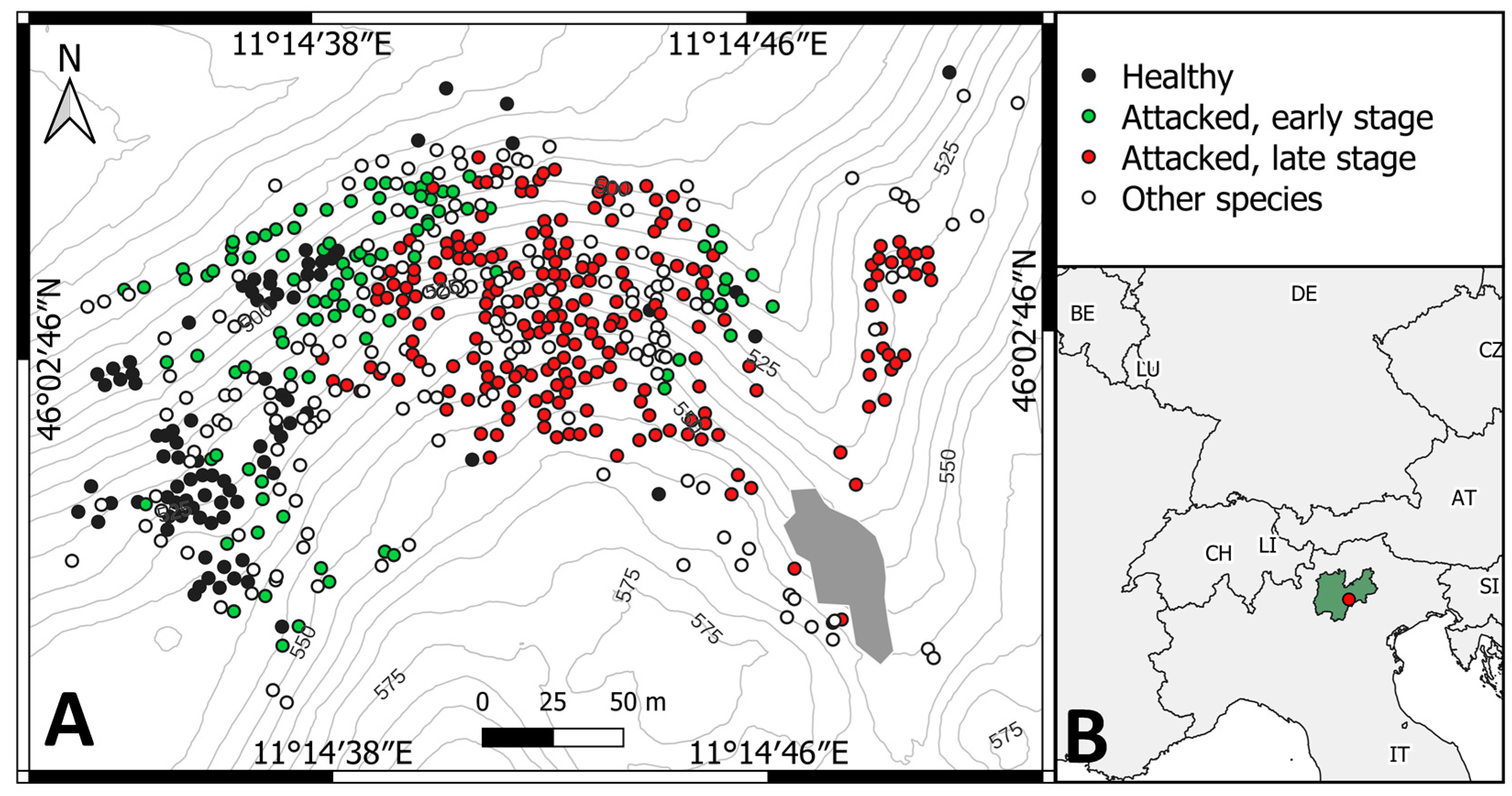
2.1.1. Study Area and Field Data

The study area is located in Northern Italy in the municipality of Pergine (Trento). It is represented by a small hill (about 10 ha, altitude range 450–570 m a.s.l.) mainly dominated by Norway spruce (Picea abies (L.) Karst.). Inside the study area a windthrow event happened at the end of October 2018 [38], and the dead trees left on the ground generated an outbreak of European spruce bark beetles. The climate of the area is classified as temperate oceanic according to the Worldwide Bioclimatic Classification System [39]. Regarding the weather conditions in the months of June, July, August and September 2020 analysed in this study, the mean maximum temperature in that area was 16.2 °C, 20.1 °C, 18.7 °C and 14.3 °C, respectively, compared to the mean maximum temperature for the period 1930–2021, with mean maximum temperatures of 16.2 °C, 19.9 °C, 19.2 °C and 15.1 °C, respectively. Concerning precipitation, the monthly precipitation values, in mm, were 108.0, 77.8, 189.4, and 35.0, respectively, compared to the mean monthly precipitation values for the period 1921–2021, which were106.5, 94.76, 95.65, and 91.27, respectively [40].
Field data collection was carried out between the last week of October and mid-November 2020: 565 trees were geolocated using a Lasertech TruePulse 360B (Laser Technology, Inc., Centennial, CO, USA) starting from multiple base stations point localized with a precise GPS. Species and health status of each tree were collected in the field. The outbreak was localized mainly on the south-facing slope of the hill. In Figure 1, a representation of the trees measured in the field is shown, and in Table 1, a summary of the field data divided by species and health status is provided. The bark beetle infestation was divided into three categories: (1) healthy (H), trees with healthy status that did not show any sign in the trunk and crown of bark beetle infestation; (2) attacked—early stage (A1), trees that showed signs of attack at early stage, ranging from bark beetle holes in the trunk without any sign in the crown, to crowns starting to lose needles or with presence of yellow needles; and (3) attacked—late stage (A2), trees with totally yellow crowns or red or grey crowns. The species different from Picea abies (L.) Karst. were all aggregated into the class “other species” (OS).

2.1.2. Remote Sensing Data
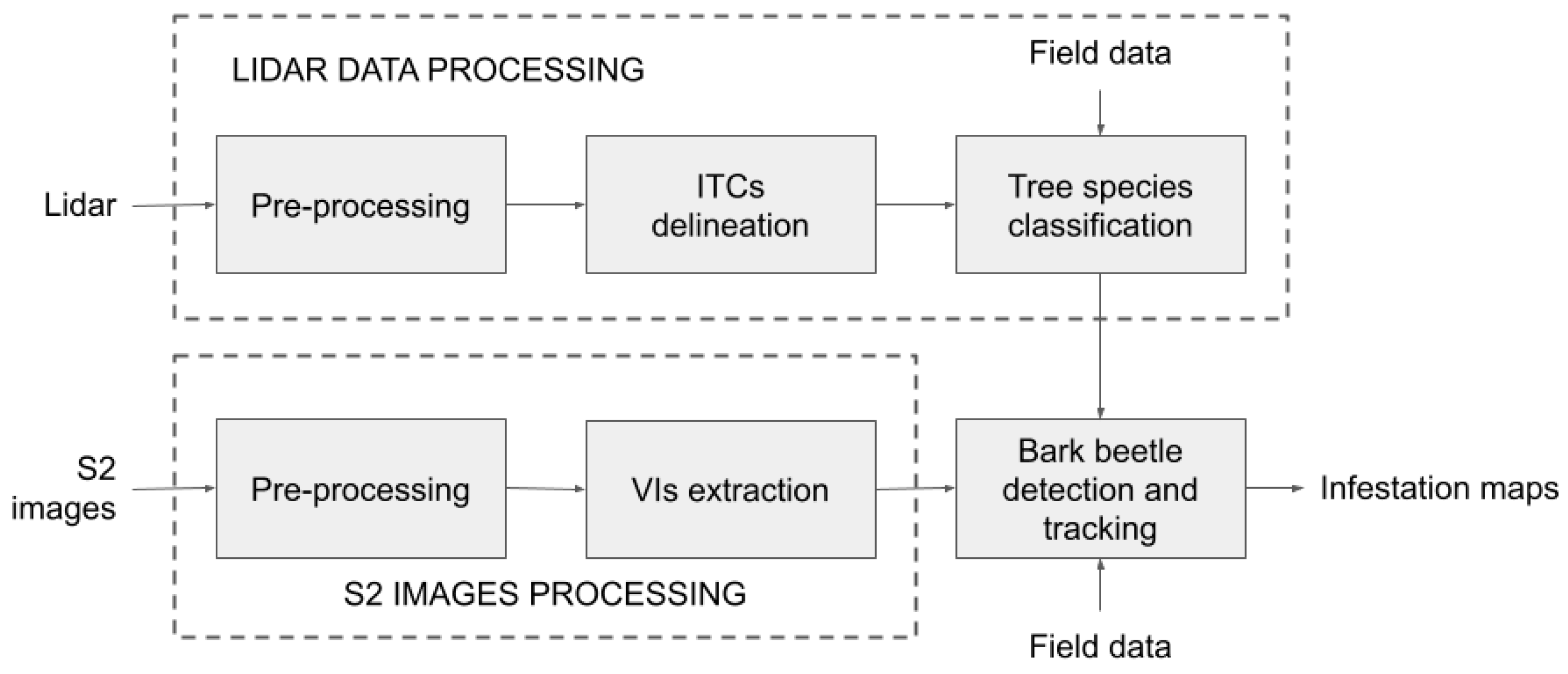
For this study, we considered multispectral satellite data acquired by the Sentinel-2 (S2) constellation and airborne lidar data. S2 is a two-satellite constellation (S2-A and S2-B) managed by the European Space Agency (ESA) under the Copernicus programme, providing high spatial resolution optical imaging every 5 days. Each S2 multispectral image is composed of 13 spectral bands at three different spatial resolutions (10 m, 20 m and 60 m [41]), but only bands at 10 m and 20 m spatial resolution were used. Lidar data were acquired over the study area in summer 2015 by an Optech ALTM 3100EA (Teledyne Optech Inc., Vaughan, ON, Canada) sensor with a maximum scan angle of 21 degrees. The mean point density was 21.5 points per square meter for the first return. Up to four returns per pulse were measured. Even though lidar data was acquired 5 years earlier than the field data, the changes in the area, apart from the windthrow event site, were limited to natural forest growth. Thus, the data can be used for ITC detection in a reliable manner.
All the available S2 cloud-free images between the 1 June 2020 and the 30 September 2020 were downloaded from the ESA portal [42] in the L2A processing level for a total of 32 images. The study area is covered by two S2 orbits, numbers 22 and 65. For the analysis of this study we selected one image about every two weeks for a total of ten images. The time distance among the images varied from 10 to 15 days with a mean of 13.3 days.

2.2. Methods

In Figure 2, the architecture of the system used to detect and monitor the bark beetle attack is presented. In the following sections, each step is detailed.

2.2.1. Lidar Data Processing

The elevation (Z) value of each lidar point was normalized with a digital terrain model (DTM) using the function normalize_height of the R package lidR [43]. The company that acquired the data provided the DTM. A calibration of the intensity value for each lidar point was performed in order to reduce the effect of the flying altitude and of the scan angle on it. We used the method of Yu et al. [44]:
I C = I * ( R R s ) α ,
where I C is the calibrated intensity, I the raw intensity, R is the sensor-to-target range and R s is the reference range or average flying height. Following the suggestions of Korpela et al. [45], an exponential factor of 2.5 was used. This is performed because environmental factors can be considered stable and the same acquisition conditions (parameters and instruments) were maintained during the survey [44].
The normalized lidar point cloud were used to delineate individual tree crowns (ITCs) by means of Dalponte and Coomes’ [46] algorithm implemented in the itcLiDAR function of the R library itcSegment. This algorithm is based on an adaptive local maxima filter and a region-growing method, and it has been successfully used in many previous studies [47,48,49,50]. The algorithm follows these steps: (1) generate a raster canopy height model (CHM) of spatial resolution defined by the user; (2) apply a Gaussian low-pass filter of fixed size of 3 × 3 pixels to the rasterized CHM in order to smooth the surface and to reduce the number of potential local maxima; (3) apply a moving window of variable size to the smoothed CHM in order to find a set of potential treetops (local maxima). The size of the window is an odd number proportional to the pixel value at the centre of the window. The range of the window size is user defined. The central pixel of the window is labelled as local maxima if its value is greater than all other values in the window while being greater than some minimum height above ground (usually fixed at 2 m); (4) iteratively analyse and add the pixels around each local maxima to the local maxima to create a region. A pixel is added to a specific region only if its vertical distance from the local maximum is less than a predefined percentage of the local maximum height and less than a predefined maximum difference. The process is repeated until no further pixels are added to any region; and (5) apply a 2D convex hull to the pixel coordinates of each region, resulting in polygons that represent ITCs. For each delineated ITC, the mean intensity value of the first return points was computed.
A link between delineated ITCs and the trees measured in the field was created by means of the method by Zhao et al. [51] that is based on Euclidean distance. As the height of the field trees was not available, only the X and Y directions were used in the computation of the distance.

2.2.2. S2 Image Processing

For each S2 image, only the bands at 10 and 20 m spatial resolution were selected, and they were all resampled at 10m with nearest neighbour resampling using the resample function of the R package raster [52]. From each image, a series of vegetation indices (VIs) were extracted (Table 2). The VIs were chosen based on the current literature. The extraction was carried out using the function spectralIndices of the R package RStoolbox [53].
Afterwards the index values were normalized: for each index, the mean value at time t of that index for the ITCs that were healthy on the 30th September 2020 ( I n d e x H e a l t h y   09 / 30 t ) was subtracted from all the ITCs and the mean value of that index over the same ITCs in the last image of the time series (30 September 2020) ( I n d e x H e a l t h y   09 / 30 09 / 30 ) was added to all the ITCs:
I n d e x N o r m t = ( I n d e x t m e a n ( I n d e x H e a l t h y   09 / 30 t ) ) + m e a n ( I n d e x H e a l t h y   09 / 30 09 / 30 ) ,
where t ranges from the first to the last image of the time series. We used the last image of the time series (30 September 2020) as reference as it was the image closest to the field data collection. This normalization step was used to remove the effect of the phenology. This is very important in order to make images at different timings comparable, otherwise the standard SVM classifier cannot be used. In principle, this can be also be performed by considering a group of Norway spruce trees that were definitely healthy for the entire time series analysis outside the area investigated but inside the image.
For each of the delineated ITCs the weighted mean of each VI was extracted. The weighted mean was performed considering the percentage of cover that each ITC had over each VIs pixel at 10m resolution. In this way we obtained one value for each index for each image for each ITC (200 values: 20 indices for 10 images).

2.2.3. Tree Species Classification and Bark Beetle Detection

Tree species classification and bark beetle attack detection were carried out using a class-weighted support vector machine (wSVM) classifier [49]. SVM is a well-known classifier that has been widely used in many studies in forestry and ecology [49,72,73,74]. Here, we chose a class-weighted version as it is more suitable for imbalanced problems such as cases where not all the classes have the same number of samples. In particular, the only difference between a standard SVM and a class-weighted SVM is that a weight, different for each class, is added inside the optimization problem of the SVM. In particular, in this study we used a weight defined in this way:
s i = max k = 1 , , Ψ ( N k ) N i ,
where N k is the number of samples that belong to the k-th class.
The feature used to train the wSVM in the tree species classification step was the mean lidar intensity of the first return points inside each ITC. We chose to use just this feature as from an initial analysis on the lidar intensity values it appeared that the Norway spruce trees were easily separable from the others. Since tree species classification is not the core of this paper, any other input feature could be used for this task.
The features used to train the wSVM for bark beetle attack detection were the vegetation indices extracted from the S2 image from the 30 September 2020. Among all the indices extracted, we considered 22 training configurations: (1) a wSVM trained using all the available indices, (2) a wSVM trained using a subset of indices selected using a feature selection method, and (3–22) a wSVM trained using each individual index separately. In these last 20 configurations, the SVM was trained with only one input feature. An SVM with only one input feature could be considered as a sort of thresholding algorithm. Though this configuration does not exploit the full potential of an SVM, we found it more important to use the same classification algorithm in all the experiments. Feature selection was carried out using a wrapper method, using the sequential floating forward selection (SFFS) [75] method as the search strategy and a separability measure for the accuracy of the wSVM classifier after a cross-validation on the training set. The SFFS method explores the possible combinations of features by testing each time the wSVM classification on the pool of features considered. It starts from one features and it stops when the increase in accuracy is insignificant. The search strategy is moving both forward and backward, as at each iteration, the selected features are reconsidered and, if unnecessary, they are discarded. This procedure was performed using the R library FSinR [76]. We chose this search strategy as it was successfully used in previous studies in the literature [49,72,73,74]. The kernel function used in the wSVM was an RBF kernel. As in every SVM classification, some parameters needed to be tuned: we tuned the cost parameter C and the RBF kernel parameter sigma. The tuning was performed using a grid search strategy of 400 combinations of C and sigma parameters.

2.2.4. Validation of the Classifications

For both the tree species classification and the bark beetle attack detection, the validation was performed using a three-fold cross-validation procedure. The three folds were created by overlapping a spatial grid of 40 m × 40 m to the study area. Each square of the grid was assigned to one of the three folds. Each ITC was assigned only to one square and all the ITCs inside a square were assigned to a fold. In this way, we ensured a spatial representation of the study area for each fold, reducing also the spatial correlation among the ITCs. We used 40 m as it is double the size of the coarser resolution of the S2 bands considered in order to eliminate the possibility of having ITCs belonging to different folds overlapping the same S2 pixels.
The classification results over the three folds were presented in terms of confusion matrix, overall accuracy (OA), balanced accuracy (BA), producer accuracy (PA) and user accuracy (UA). We also considered the BA as an overall metric defined as the average of the PAs, as the classification problem is unbalanced and thus analysing only the OA is not the optimal choice. The final map was validated with a confusion matrix and the corresponding accuracies computed by matching the ITCs classified into four classes (OS, H, A1 and A2) with the field dataset.

2.2.5. Multitemporal Tracking of the Bark Beetle Infestation

Among all the bark beetle attack classification models, we chose the best one and we applied it to the 10 S2 images from the 2 June 2020 to the 30 September 2020. The wSVM model used was trained on the S2 image of the 30 September 2020. The rationale for this step is to track the bark beetle infestation over time and to understand how it spreads in the forest. These maps were studied at two levels: (1) the differences among two consecutive maps were analysed in order to detect reasonable and unreasonable changes; and (2) the time behaviour of the infestation of each Norway spruce ITC was analysed in order to evaluate whether it was following a reasonable trend or not. Concerning the first one, the differences between two consecutive maps were analysed on the basis of some rules according to the type of change/transition that could actually happen between times t 1 and t 2 [77,78], with t 1 indicating the status of an ITC at time 1 and t 2 the status of an ITC at time 2, where time 2 is the time period just after time 1. The changes/transitions considered are as follows: (1) reasonable change, when the infestation stage remains the same or moves forward (e.g., from H to A1) and (2) unreasonable change, when the infestation stage moves backward instead of forward (e.g., from A2 to H). In Table 3, the detailed set of rules and the types of changes are summarized.
Regarding the time behaviour of each ITC, we considered seven possible reasonable situations: (1) an ITC is classified as H in all the 10 maps considered; (2) an ITC is classified as A1 in all the 10 maps considered; (3) an ITC is classified as A2 in all the 10 maps considered; (4) an ITC is classified for one or more consecutive maps as H, followed by one or more consecutive maps as A1; (5) an ITC is classified for one or more consecutive maps as H, followed by one or more consecutive maps as A2; (6) an ITC is classified for one or more consecutive maps as H, followed by one or more consecutive maps as A1, followed by one or more consecutive maps as A2; and (7) an ITC is classified for one or more consecutive maps as A1, followed by one or more consecutive maps as A2.

3. Results

3.1. ITC Detection and Tree Species Classification

Regarding the ITC detection, out of 565 trees measured in the field, 512 were matched with a delineated ITC, reaching a 90% detection rate. Among the matched ITCs, 368 were Norway spruce, while the remaining were other species. Concerning the status of the bark beetle outbreak, among the Norway spruce–matched ITCs we had 76 ITCs in class H, 87 in class A1, and 205 in class A2.
The tree species classification was obtained with an OA of 87.4% and a BA of 82.8%. Overall, the results were good, providing PAs and UAs over 70%. The confusion matrix for the best combination of wSVM parameters over the three folds is shown in Table 4, along with the PAs and UAs.

3.2. Bark Beetle Detection

Balanced accuracies obtained using the wSVM with the threefold cross-validation for the bark beetle attack classification, from the image from the 30th of September 2020, are shown in Figure 3. Using the subset of indices obtained using the feature selection algorithm (FS model), we obtained the highest balanced accuracy (BA = 72.9%; OA = 73.6%). The feature selection algorithm selected eight indices for the classification: CLRE, GNDVI, NBRI, NDREI2, NDVI, NRVI, REIP and SLAVI. The second best result in terms of BA was obtained using the CLRE index (BA = 71.3%; OA = 72.3%), while the model using all the available indices was the fourth best (BA = 68.5%; OA = 70.1%). Considering the FS model (the one with the subset of indices), we obtained PAs of 76.3% (H class), 66.7% (A1 class) and 75.6% (A2 class) and UAs of 65.9% (H class), 53.2% (A1 class) and 90.6% (A2 class). The confusion matrices for the abovementioned three models (FS, CLRE and all) are shown in Table 5.

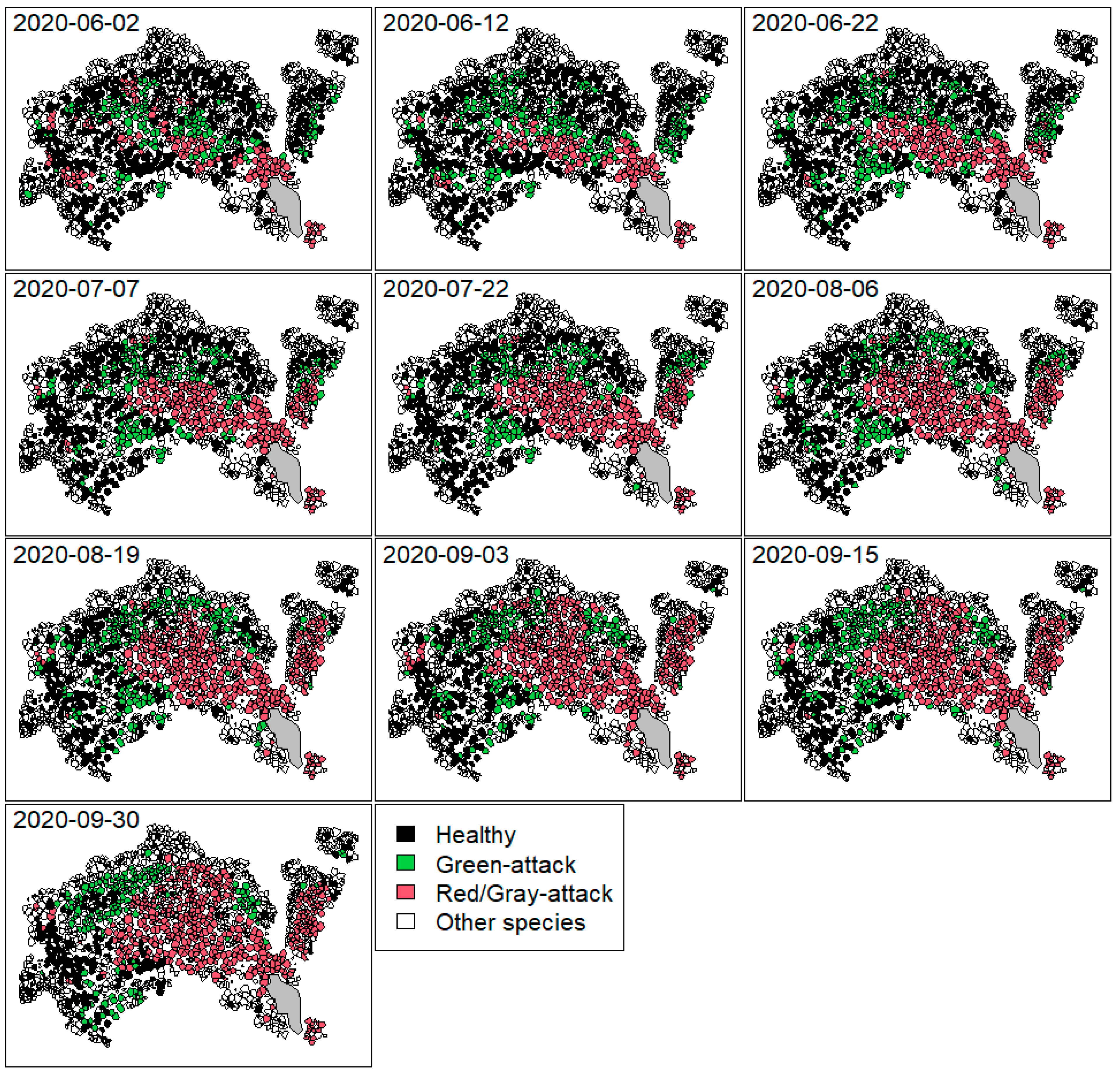
3.3. Mapping Bark Beetle Presence and Tracking it in Time

Using the wSVM model based on the features selected by the feature selection method, we generated a map of the area for the 30 September 2020 (Figure 4). We chose the model based on a subset of features (FS model) as it was the one providing the highest BA. This map was based on four classes (i.e., H, A1, A2, OS) as the map is the combination of both the tree species classification and the bark beetle classification processes. The OA of the final map was 79.2% and the balanced accuracy was 77.6%. In Table 6, the confusion matrix is shown.
Using the same model, we classified all the 10 S2 images considered in order to generate maps that track the evolution of the infestation (Figure 5). As explained in the methods section, the exploration of the multitemporal maps was performed at two levels. Concerning the comparisons among two consecutive maps, they were analysed on the basis of reasonable and unreasonable changes in time. As it can be seen in Table 7, the reasonable change detection rate is, on average, 88%, with a maximum of 91.3% between the maps of the 12 and 22 June 2020. Regarding the analysis of the entire time series, 72.1% of the ITCs showed a behaviour that could be considered reasonable according to the rules explained in Section 2.2.4, 16.9% of the ITCs showed an unreasonable behaviour, while 11.1% of the ITCs showed an unreasonable behaviour but only because one map (out of ten) was wrong.

4. Discussion

Detecting the earliest stages of bark beetle outbreaks is, without doubt, of great relevance since it allows for decision makers to act and stop the propagation of the infestation on time. In fact, some studies have been carried out in the literature with the goal of detecting early stage attacks from different approaches: classification, index analysis, bi-temporal data and yearly analysis and early detection [14,28,30,33,79]. Even though these studies were able to detect early stage attacks, their accuracy varied a lot and was sensor-dependent in the sense that they required working with a very high spatial resolution (VHR). Obtaining access to VHR data is not free and thus lowers the possibility of actually detecting the bark beetle outbreak.
In this paper, we explored the possibility of combing lidar and S2 data for the detection of the different stages of the outbreak (i.e., early and late) as well as for tracking the evolution of the outbreak in time. Firstly, we showed that by combining S2 data with ITCs delineated on lidar data, it is possible to have very spatially detailed maps. Such maps are intended to provide more accurate information for forest management purposes. Secondly, we evaluated the performance of several spectral indices (among which were the most used in the literature for bark beetle detection) to detect the early stage of the infestation, and we identified the best one in terms of balanced accuracy. Lastly, we presented a strategy to track the infestation over time by introducing a set of rules that allow us to check the veracity of the detection, even without reference data. From an ecological point of view, this opens the path to further studies related to the behaviour of bark beetles and the dynamics of how they spread in a forest.

4.1. Infestation Detection at ITCs Level

Norway spruce trees are the ones mainly affected by bark beetle insects and should therefore be classified beforehand. For this paper, such classification was performed using only lidar data, obtaining an OA of 87.4%, BA of 82.8% and a PA for the Norway spruce trees of 74.0%. The classification for bark beetle detection provided an OA of 73.6% and a BA of 72.9%, with a PA for the early stage attack (A1) of 66.7%. Combining the Norway spruce classification with that for the bark beetle, we obtained a map that, with all the available field data, reached an OA of 79.2%, a BA of 77.6% and a PA for the early stage attack (A1) of 77.0%. Such a PA value for the early attack stage is relevant for two main reasons: (1) we are mapping tree information using S2 data, for which the spatial resolution is larger than actual ITC size; and (2) knowing the location of the early stage attack can help to remove or reduce the propagation of the infestation in time. The combination of the two classifications helped to reduce false alarms present in areas where bark beetle infestation could not happen, thereby improving the final map.

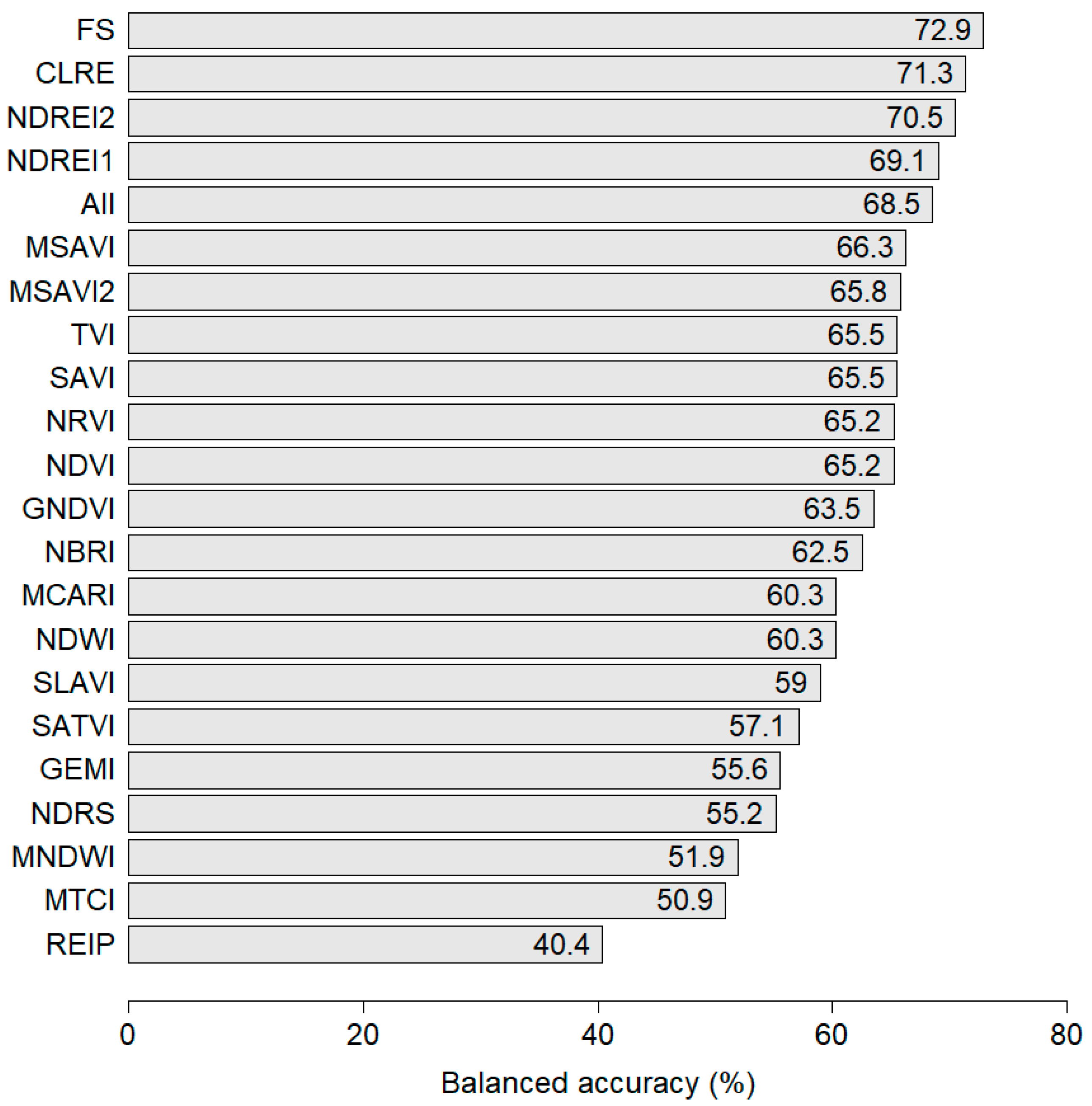
4.2. Identification of the Most Robust Spectral Index

An important part that has been widely addressed in literature is the proper selection of spectral indices to be used [21,28,29]. Here we selected the indices using a sub-optimal search strategy (the SFFS one) that allowed us a good trade off among execution time and the quality of the selected indices in terms of information provided for class separability. Nevertheless, we are sure that the selected indices provide accurate information about the trees’ states due to the spectral bands used to derive them (other than the high accuracy obtained). Most of them make use of a NIR, SWIR and/or Red Edge band. Such bands have been found in the literature [18] to be suitable for studying stressed or healthy trees or forest areas. While indices such as the NDREI2 and the NDRS have been reported as the best in the literature for detecting the different stages of bark beetle infestation, it was found that NDREI1 performs nearly equally to the CLRE and NDREI2 indices (see Figure 3 for more details), with a BA of 69.1% vs. 71.3% and 70.5%, respectively. In contrast, NDRS performed among the five worst indices with a BA of only 55.2%. A further analysis, by combining several indices, was also performed that allowed us to identify eight indices as the best ones for performing the detection task, with a balanced accuracy of 72.9%. Combining all indices in Table 2 offered the fifth best performance with a BA of 68.5%, allowing us to see how sensor- and location-dependent this analysis can be. It was also possible to prove the relevance of performing a detailed analysis of the most frequently used indices according to specific needs.

4.3. Detection of Early Stage Attack

The detection of the early stage attack was performed with a machine learning approach and by combining both species classification and the bark beetle infestation itself. While a formal comparison to other state-of-the-art methods is not offered in this paper, it is important to recall that other studies can be found in the literature that have addressed early stage–attack detection analysis [14,28,30,33,79], though from different perspectives. Huo et al. [33] and Bárta et al. [14] have exploited the S2 time series, covering the period April–October of 2018 and 2019, in order to detect stressed trees (a tree can be stressed for several reasons and not only because of the presence of bark beetles) that could lead to the early detection of bark beetle infestations but cannot guarantee the actual detection of an early stage attack itself. Huo et al. [33] proposed a new vegetation index called the Normalized Distance Red and SWIR (NDRS) that allowed them to detect stressed trees, with accuracies ranging from 82 to 86%. Bárta et al. [14] made use of several indices, in particular the well-known tasseled cap ones, in order to monitor the evolution of healthy and infected trees during a year and perform early detection of bark beetle infestation with an accuracy of 78%. These two studies are the most recent ones available in the literature; yet, multitemporal information is not used as a tool to track or detect infestation evolution but to detect stressed trees. Observed trees can be stressed for several reasons and not only due to the presence of bark beetle insects. Therefore, detecting the early stage of the attack itself is more crucial and can better help to prevent the spread of infestation, without cutting off actual healthy trees.

4.4. Attack Evolution Monitoring

Looking at the temporal classification maps shown in Figure 5, it is clear how performing an analysis over a more complete and regular time series can allow the tracking of the bark beetle outbreak’s evolution. Even though there is no field data collected for each of the different maps, it is clear how, starting from a classification map obtained with actual field data for the last month and then going back in time, it is possible to actually track the evolution of the bark beetle infestation. In fact, the image corresponding to the 30th of September already shows a clear and close result to that of the actual field data for October 2020 (see Figure 1). On the other hand, knowing the location of the windthrow event (as well as any other possible event happening in the study area) helps to understand where the infestation originated from or whether there was any accelerating process for the infestation. By June 2020, the bark beetle attack had already gone out of control since nearly two years had passed since the windthrow event, showing clear signs of an attack in the late stage. Such cases, together with the knowledge about the study area/region, allow us to qualitatively corroborate the truthfulness of our results. In order to perform a sort of quantitative analysis without the availability of the ground truth for every single date, the set of rules in Table 3 was introduced. These rules take inspiration from land cover map updates, where reliable change rules allow understanding, as compared with knowing whether those from a new class are possible or not after a certain time [80]. Such is the case for the H, A1 and A2 stages that can only happen in this same direction and not in the opposite one. Since we have the ground truth for the last acquisition date, we can track the evolution of the different stages by checking the defined rules in order to evaluate the multitemporal accuracy detection. Table 7 summarizes the results for all the cases, where the reasonable prediction varies from 85.0 to 91.3%. A final check was made by studying the time behaviour according to seven possible steadiness situations. In this case, it was found that nearly 72.1% of the ITCs kept a reasonable trend across the studied period, with only 16.8% of ITCs showing some major errors. Of particular interest are the 11.1% of ITCs that presented an error only on one of the dates. This means that we are facing cases of weak false alarms that could be easily corrected by means of this same strategy (by checking these samples with the established rules and changing the classification value to a logical one). Nevertheless, we preferred to keep the original data in order to show the possible readers the high accuracy achieved by the proposed approach. Such results allow us to further prove the reliability of the proposed approach as well as to show how it is possible to accurately track the attack’s evolution in time. In this way, it is not only possible to detect the attack in an early stage in an accurate way but possibly to track it in images acquired after the field data collection. This last part is concluded from the temporal distribution of the analysed images. It is important to note that the monitoring analysis could not be carried out just the day after a windthrow event happens. This is because it takes some time for bark beetles to start attacking the affected trees and thus spread to other healthy trees.

4.5. Limitations

While the presented approach is promising and able to produce reliable and useful results, limitations exist that arise from the spatial resolution itself. Working with Sentinel-2 data means we are working at 10 m × 10 m pixels. Such an area could cover more than a single tree, especially if considering young trees that are just starting to grow. Indeed, it was found that 55.4% of the ITCs had VI values not duplicated with other ITCs, whereas 44.6% of the ITCs had duplicated values. Looking at the sizes of such trees, it is immediately visible that duplicated ones are generally trees with smaller crowns compared to non-duplicated ones. This means that our method is able to properly monitor large trees, while it has problems monitoring smaller ones. Yet, the presented results show that the proposed method is able to accurately map bark beetle outbreaks at a low cost.

5. Conclusions

In this study we showed that it is possible to accurately detect a bark beetle attack in early and late stages at the ITCs level using multispectral satellite data by means of a machine learning classification approach. Furthermore, we also showed that the use of multitemporal data allows tracking of the evolution of the bark beetle infestation with a bi-weekly resolution. The possibility of monitoring the outbreak using freely available S2 data is extremely important as it allows an almost real-time mapping (not at an economical cost) and consequently rapid interventions. Additionally, maps at ITC level (extracted by lidar data that nowadays are available by public administrations in many countries) allow a spatially detailed map of the outbreak evolution and a punctual intervention by forest managers. Indeed, from a management point of view, the possibility to detect the attack at an early stage is very important as it allows planning the harvesting in order to stop the attack and minimize economic losses.
As future developments, it would be interesting to make use of sensors with higher spatial resolution, such as Dove/Planet constellation, in order to perform a more detailed ITCs analysis. Even though the oldest generation of Dove/Planet does not come with a red edge band, which in this study and many others emerged to be quite relevant in the proper detection of bark beetle attack stages, the newest generation (since 2019) does come with such information [81]. Thus, working with higher spatial resolution sensors would allow for further studying the impact of multitemporal information on bark beetle infestation monitoring.

Author Contributions

Conceptualization, M.D.; methodology, M.D. and Y.T.S.-C.; software, M.D.; validation, M.D. and L.F.; formal analysis, M.D. and Y.T.S.-C.; investigation, M.D. and Y.T.S.-C.; data curation, M.D. and L.F.; writing—original draft preparation, M.D. and Y.T.S.-C.; writing—review and editing, M.D., Y.T.S.-C. and D.G.; visualization, M.D.; supervision, D.G. All authors have read and agreed to the published version of the manuscript.

Funding

This work was funded by the Highlander project co-financed by the Connecting European Facility Programme of the European Union Grant agreement n° INEA/CEF/ICT/A2018/1815462.

Data Availability Statement

Data available on request to the corresponding author.

Acknowledgments

The authors would like to thank the Autonomous Province of Trento (Italy) for providing the lidar data used in this study.

Conflicts of Interest

The authors declare no conflict of interest.

References

  1. Wermelinger, B. Ecology and Management of the Spruce Bark Beetle Ips Typographus—A Review of Recent Research. For. Ecol. Manag. 2004, 202, 67–82. [Google Scholar] [CrossRef]
  2. Forzieri, G.; Girardello, M.; Ceccherini, G.; Spinoni, J.; Feyen, L.; Hartmann, H.; Beck, P.S.A.; Camps-Valls, G.; Chirici, G.; Mauri, A.; et al. Emergent Vulnerability to Climate-Driven Disturbances in European Forests. Nat. Commun. 2021, 12, 1081. [Google Scholar] [CrossRef]
  3. Cook, E.R.; Zedaker, S.M. The Dendroecology of Red Spruce Decline. In Ecology and Decline of Red Spruce in the Eastern United States; Eagar, C., Adams, M.B., Eds.; Ecological Studies; Springer: New York, NY, USA, 1992; pp. 192–231. ISBN 978-1-4612-2906-3. [Google Scholar]
  4. Eagar, C.; Adams, M.B. (Eds.) Ecology and Decline of Red Spruce in the Eastern United States; Ecological Studies; Springer: New York, NY, USA, 1992; ISBN 978-0-387-97786-7. [Google Scholar]
  5. Scott, J.T.; Siccama, T.G.; Johnson, A.H.; Breisch, A.R. Decline of Red Spruce in the Adirondacks, New York. Bull. Torrey Bot. Club 1984, 111, 438–444. [Google Scholar] [CrossRef]
  6. Biedermann, P.H.W.; Müller, J.; Grégoire, J.-C.; Gruppe, A.; Hagge, J.; Hammerbacher, A.; Hofstetter, R.W.; Kandasamy, D.; Kolarik, M.; Kostovcik, M.; et al. Bark Beetle Population Dynamics in the Anthropocene: Challenges and Solutions. Trends Ecol. Evol. 2019, 34, 914–924. [Google Scholar] [CrossRef] [Green Version]
  7. Southern Pine Beetle Suppression Strategy in Southeastern U.S.: Environmental Impact Statement; Northwestern University: Evanston, IL, USA, 1974.
  8. Cailleret, M.; Nourtier, M.; Amm, A.; Durand-Gillmann, M.; Davi, H. Drought-Induced Decline and Mortality of Silver Fir Differ among Three Sites in Southern France. Ann. For. Sci. 2014, 71, 643–657. [Google Scholar] [CrossRef]
  9. Niemann, K.O.; Visintini, F. Assessment of Potential for Remote Sensing Detection of Bark Beetle-Infested Areas during Green Attack: A Literature Review; Mountain Pine Beetle Initiative Working Paper 2005-02; Natural Resources Canada; Canadian Forest Service; Pacific Forestry Centre: Victoria, BC, Canada, 2005.
  10. Weng, Q. Remote Sensing for Sustainability, 1st ed.; Taylor & Francis: Abingdon, UK, 2019; ISBN 978-0-367-87140-6. [Google Scholar]
  11. White, J.; Wulder, M.; Brooks, D.; Reich, R.; Wheate, R. Detection of Red Attack Stage Mountain Pine Beetle Infestation with High Spatial Resolution Satellite Imagery. Remote Sens. Environ. 2005, 96, 340–351. [Google Scholar] [CrossRef]
  12. Wulder, M.A.; Dymond, C.C.; White, J.C.; Leckie, D.G.; Carroll, A.L. Surveying Mountain Pine Beetle Damage of Forests: A Review of Remote Sensing Opportunities. For. Ecol. Manag. 2006, 221, 27–41. [Google Scholar] [CrossRef]
  13. Skakun, R.S.; Wulder, M.A.; Franklin, S.E. Sensitivity of the Thematic Mapper Enhanced Wetness Difference Index to Detect Mountain Pine Beetle Red-Attack Damage. Remote Sens. Environ. 2003, 86, 433–443. [Google Scholar] [CrossRef]
  14. Bárta, V.; Lukeš, P.; Homolová, L. Early Detection of Bark Beetle Infestation in Norway Spruce Forests of Central Europe Using Sentinel-2. Int. J. Appl. Earth Obs. Geoinf. 2021, 100, 102335. [Google Scholar] [CrossRef]
  15. Hlásny, T.; König, L.; Krokene, P.; Lindner, M.; Montagné-Huck, C.; Müller, J.; Qin, H.; Raffa, K.F.; Schelhaas, M.-J.; Svoboda, M.; et al. Bark Beetle Outbreaks in Europe: State of Knowledge and Ways Forward for Management. Curr. For. Rep. 2021, 7, 138–165. [Google Scholar] [CrossRef]
  16. Solano-Correa, Y.T.; Carcereri, D.; Bovolo, F.; Bruzzone, L. Identification of Non-Photosynthetic Vegetation Areas in Sentinel-2 Satellite Image Time Series. In Proceedings of the SPIE Remote Sensing: Image and Signal Processing for Remote Sensing XXV, Strasbourg, France, 9–12 September 2019; Volume 11155, p. 111550Y. [Google Scholar]
  17. Solano-Correa, Y.T.; Bovolo, F.; Bruzzone, L.; Fernández-Prieto, D. Automatic Derivation of Cropland Phenological Parameters by Adaptive Non-Parametric Regression of Sentinel-2 NDVI Time Series. In Proceedings of the IGARSS 2018, Valencia, Spain, 22–27 July 2018; pp. 1946–1949. [Google Scholar]
  18. Lausch, A.; Heurich, M.; Gordalla, D.; Dobner, H.-J.; Gwillym-Margianto, S.; Salbach, C. Forecasting Potential Bark Beetle Outbreaks Based on Spruce Forest Vitality Using Hyperspectral Remote-Sensing Techniques at Different Scales. For. Ecol. Manag. 2013, 308, 76–89. [Google Scholar] [CrossRef]
  19. Fernandez-Carrillo, A.; Patočka, Z.; Dobrovolný, L.; Franco-Nieto, A.; Revilla-Romero, B. Monitoring Bark Beetle Forest Damage in Central Europe. A Remote Sensing Approach Validated with Field Data. Remote Sens. 2020, 12, 3634. [Google Scholar] [CrossRef]
  20. Franklin, S.E.; Wulder, M.A.; Skakun, R.S.; Carroll, A.L. Mountain Pine Beetle Red-Attack Forest Damage Classification Using Stratified Landsat TM Data in British Columbia, Canada. Photogramm. Eng. Remote Sens. 2003, 69, 283–288. [Google Scholar] [CrossRef]
  21. Havašová, M.; Bucha, T.; Ferenčík, J.; Jakuš, R. Applicability of a Vegetation Indices-Based Method to Map Bark Beetle Outbreaks in the High Tatra Mountains. Ann. For. Res. 2015, 58, 295–310. [Google Scholar] [CrossRef]
  22. Wulder, M.A.; White, J.C.; Bentz, B.; Alvarez, M.F.; Coops, N.C. Estimating the Probability of Mountain Pine Beetle Red-Attack Damage. Remote Sens. Environ. 2006, 101, 150–166. [Google Scholar] [CrossRef]
  23. Yang, S. Detecting Bark Beetle Damage with Sentinel-2 Multi-Temporal Data in Sweden. Master’s Thesis, Lund University, Lund, Sweden, 2019. [Google Scholar]
  24. Bárta, V.; Hanuš, J.; Dobrovolný, L.; Homolová, L. Comparison of Field Survey and Remote Sensing Techniques for Detection of Bark Beetle-Infested Trees. For. Ecol. Manag. 2022, 506, 119984. [Google Scholar] [CrossRef]
  25. Hellwig, F.M.; Stelmaszczuk-Górska, M.A.; Dubois, C.; Wolsza, M.; Truckenbrodt, S.C.; Sagichewski, H.; Chmara, S.; Bannehr, L.; Lausch, A.; Schmullius, C. Mapping European Spruce Bark Beetle Infestation at Its Early Phase Using Gyrocopter-Mounted Hyperspectral Data and Field Measurements. Remote Sens. 2021, 13, 4659. [Google Scholar] [CrossRef]
  26. Coops, N.C.; Johnson, M.; Wulder, M.A.; White, J.C. Assessment of QuickBird High Spatial Resolution Imagery to Detect Red Attack Damage Due to Mountain Pine Beetle Infestation. Remote Sens. Environ. 2006, 103, 67–80. [Google Scholar] [CrossRef]
  27. White, J.C.; Coops, N.C.; Hilker, T.; Wulder, M.A.; Carroll, A.L. Detecting Mountain Pine Beetle Red Attack Damage with EO-1 Hyperion Moisture Indices. Int. J. Remote Sens. 2007, 28, 2111–2121. [Google Scholar] [CrossRef]
  28. Abdullah, H.; Skidmore, A.K.; Darvishzadeh, R.; Heurich, M. Sentinel-2 Accurately Maps Green-Attack Stage of European Spruce Bark Beetle (Ips typographus, L.) Compared with Landsat-8. Remote Sens. Ecol. Conserv. 2019, 5, 87–106. [Google Scholar] [CrossRef] [Green Version]
  29. Abdullah, H.; Skidmore, A.K.; Darvishzadeh, R.; Heurich, M. Timing of Red-Edge and Shortwave Infrared Reflectance Critical for Early Stress Detection Induced by Bark Beetle (Ips typographus, L.) Attack. Int. J. Appl. Earth Obs. Geoinf. 2019, 82, 101900. [Google Scholar] [CrossRef]
  30. Abdullah, H.; Darvishzadeh, R.; Skidmore, A.K.; Heurich, M. Sensitivity of Landsat-8 OLI and TIRS Data to Foliar Properties of Early Stage Bark Beetle (Ips typographus, L.) Infestation. Remote Sens. 2019, 11, 398. [Google Scholar] [CrossRef] [Green Version]
  31. Gomez, D.F.; Ritger, H.M.W.; Pearce, C.; Eickwort, J.; Hulcr, J. Ability of Remote Sensing Systems to Detect Bark Beetle Spots in the Southeastern US. Forests 2020, 11, 1167. [Google Scholar] [CrossRef]
  32. Goodwin, N.R.; Magnussen, S.; Coops, N.C.; Wulder, M.A. Curve Fitting of Time-Series Landsat Imagery for Characterizing a Mountain Pine Beetle Infestation. Int. J. Remote Sens. 2010, 31, 3263–3271. [Google Scholar] [CrossRef]
  33. Huo, L.; Persson, H.J.; Lindberg, E. Early Detection of Forest Stress from European Spruce Bark Beetle Attack, and a New Vegetation Index: Normalized Distance Red & SWIR (NDRS). Remote Sens. Environ. 2021, 255, 112240. [Google Scholar] [CrossRef]
  34. Liang, L.; Chen, Y.; Hawbaker, T.; Zhu, Z.; Gong, P. Mapping Mountain Pine Beetle Mortality through Growth Trend Analysis of Time-Series Landsat Data. Remote Sens. 2014, 6, 5696–5716. [Google Scholar] [CrossRef] [Green Version]
  35. Meddens, A.J.H.; Hicke, J.A. Spatial and Temporal Patterns of Landsat-Based Detection of Tree Mortality Caused by a Mountain Pine Beetle Outbreak in Colorado, USA. For. Ecol. Manag. 2014, 322, 78–88. [Google Scholar] [CrossRef]
  36. Senf, C.; Pflugmacher, D.; Wulder, M.A.; Hostert, P. Characterizing Spectral–Temporal Patterns of Defoliator and Bark Beetle Disturbances Using Landsat Time Series. Remote Sens. Environ. 2015, 170, 166–177. [Google Scholar] [CrossRef]
  37. Ye, S.; Rogan, J.; Zhu, Z.; Hawbaker, T.J.; Hart, S.J.; Andrus, R.A.; Meddens, A.J.H.; Hicke, J.A.; Eastman, J.R.; Kulakowski, D. Detecting Subtle Change from Dense Landsat Time Series: Case Studies of Mountain Pine Beetle and Spruce Beetle Disturbance. Remote Sens. Environ. 2021, 263, 112560. [Google Scholar] [CrossRef]
  38. Dalponte, M.; Marzini, S.; Solano-Correa, Y.T.; Tonon, G.; Vescovo, L.; Gianelle, D. Mapping Forest Windthrows Using High Spatial Resolution Multispectral Satellite Images. Int. J. Appl. Earth Obs. Geoinf. 2020, 93, 102206. [Google Scholar] [CrossRef]
  39. Sboarina, C.; Cescatti, A. II Clima Del Trentino–Distribuzione Spaziale Delle Principali Variabili Climatiche [The Climate of Trentino–Spatial Distribution of the Principal Climatic Variables]; Report 33; Centro di Ecologia Alpina, Viote del Monte Bondone: Trento, Italy, 2004. [Google Scholar]
  40. Meteotrentino. Available online: http://storico.meteotrentino.it/web.htm?ppbm=T0409&rs&1&df (accessed on 14 June 2022).
  41. ESA, S.-2 Spatial—Resolutions—Sentinel-2 MSI—User Guides—Sentinel Online—Sentinel Online. Available online: https://sentinels.copernicus.eu/web/sentinel/user-guides/sentinel-2-msi/resolutions/spatial (accessed on 4 August 2021).
  42. Open Access Hub. Available online: https://scihub.copernicus.eu/ (accessed on 15 March 2021).
  43. Roussel, J.R.; Auty, D.; Coops, N.C.; Tompalski, P.; Goodbody, T.R.; Meador, A.S.; Bourdon, J.F.; De Boissieu, F.; Achim, A. LidR: Airborne LiDAR Data Manipulation and Visualization for Forestry Applications. Remote Sens. Environ. 2020, 251, 1120612021. [Google Scholar]
  44. Yu, X.; Hyyppä, J.; Litkey, P.; Kaartinen, H.; Vastaranta, M.; Holopainen, M. Single-Sensor Solution to Tree Species Classification Using Multispectral Airborne Laser Scanning. Remote Sens. 2017, 9, 108. [Google Scholar] [CrossRef] [Green Version]
  45. Korpela, I.; Ørka, H.O.; Hyyppä, J.; Heikkinen, V.; Tokola, T. Range and AGC Normalization in Airborne Discrete-Return LiDAR Intensity Data for Forest Canopies. ISPRS J. Photogramm. Remote Sens. 2010, 65, 369–379. [Google Scholar] [CrossRef]
  46. Dalponte, M.; Coomes, D.A. Tree-Centric Mapping of Forest Carbon Density from Airborne Laser Scanning and Hyperspectral Data. Methods Ecol. Evol. 2016, 7, 1236–1245. [Google Scholar] [CrossRef] [Green Version]
  47. Dalponte, M.; Frizzera, L.; Gianelle, D. How to Map Forest Structure from Aircraft, One Tree at a Time. Ecol. Evol. 2018, 8, 5611–5618. [Google Scholar] [CrossRef]
  48. Dalponte, M.; Frizzera, L.; Ørka, H.O.; Gobakken, T.; Næsset, E.; Gianelle, D. Predicting Stem Diameters and Aboveground Biomass of Individual Trees Using Remote Sensing Data. Ecol. Indic. 2018, 85, 367–376. [Google Scholar] [CrossRef]
  49. Nguyen, H.M.; Demir, B.; Dalponte, M. A Weighted SVM-Based Approach to Tree Species Classification at Individual Tree Crown Level Using LiDAR Data. Remote Sens. 2019, 11, 2948. [Google Scholar] [CrossRef] [Green Version]
  50. Versace, S.; Gianelle, D.; Frizzera, L.; Tognetti, R.; Garfì, V.; Dalponte, M. Prediction of Competition Indices in a Norway Spruce and Silver Fir-Dominated Forest Using Lidar Data. Remote Sens. 2019, 11, 2734. [Google Scholar] [CrossRef] [Green Version]
  51. Zhao, K.; Suarez, J.C.; Garcia, M.; Hu, T.; Wang, C.; Londo, A. Utility of Multitemporal Lidar for Forest and Carbon Monitoring: Tree Growth, Biomass Dynamics, and Carbon Flux. Remote Sens. Environ. 2018, 204, 883–897. [Google Scholar] [CrossRef]
  52. Hijmans, R.J.; Etten, J.V.; Sumner, M.; Cheng, J.; Baston, D.; Bevan, A.; Bivand, R.; Busetto, L.; Canty, M.; Fasoli, B.; et al. Raster: Geographic Data Analysis and Modeling. Available online: https://cran.r-project.org/web/packages/raster/index.html (accessed on 22 June 2022).
  53. Leutner, B.; Horning, N.; Schwalb-Willmann, J.; Hijmans, R.J. RStoolbox: Tools for Remote Sensing Data Analysis. Available online: https://cran.r-project.org/web/packages/RStoolbox/index.html (accessed on 22 June 2022).
  54. Gitelson, A.A.; Gritz, Y.; Merzlyak, M.N. Relationships between Leaf Chlorophyll Content and Spectral Reflectance and Algorithms for Non-Destructive Chlorophyll Assessment in Higher Plant Leaves. J. Plant Physiol. 2003, 160, 271–282. [Google Scholar] [CrossRef]
  55. Pinty, B.; Verstraete, M.M. GEMI: A Non-Linear Index to Monitor Global Vegetation from Satellites. Vegetatio 1992, 101, 15–20. [Google Scholar] [CrossRef]
  56. Gitelson, A.A.; Merzlyak, M.N. Remote Sensing of Chlorophyll Concentration in Higher Plant Leaves. Adv. Space Res. 1998, 22, 689–692. [Google Scholar] [CrossRef]
  57. Daughtry, C.S.T.; Walthall, C.L.; Kim, M.S.; de Colstoun, E.B.; McMurtrey, J.E. Estimating Corn Leaf Chlorophyll Concentration from Leaf and Canopy Reflectance. Remote Sens. Environ. 2000, 74, 229–239. [Google Scholar] [CrossRef]
  58. Xu, H. Modification of Normalised Difference Water Index (NDWI) to Enhance Open Water Features in Remotely Sensed Imagery. Int. J. Remote Sens. 2006, 27, 3025–3033. [Google Scholar] [CrossRef]
  59. Qi, J.; Chehbouni, A.; Huete, A.R.; Kerr, Y.H.; Sorooshian, S. A Modified Soil Adjusted Vegetation Index. Remote Sens. Environ. 1994, 48, 119–126. [Google Scholar] [CrossRef]
  60. Dash, J.; Curran, P.J. The MERIS Terrestrial Chlorophyll Index. Int. J. Remote Sens. 2004, 25, 5403–5413. [Google Scholar] [CrossRef]
  61. García, M.J.L.; Caselles, V. Mapping Burns and Natural Reforestation Using Thematic Mapper Data. Geocarto Int. 1991, 6, 31–37. [Google Scholar] [CrossRef]
  62. Gitelson, A.; Merzlyak, M.N. Spectral Reflectance Changes Associated with Autumn Senescence of Aesculus Hippocastanum L. and Acer Platanoides L. Leaves. Spectral Features and Relation to Chlorophyll Estimation. J. Plant Physiol. 1994, 143, 286–292. [Google Scholar] [CrossRef]
  63. Barnes, E.; Clarke, T.; Richards, S.; Colaizzi, P.; Haberland, J.; Kortrzewski, M.; Waller, P.; Choi, C.; Riley, E.; Thompson, T.; et al. Coincident Detection of Crop Water Stress, Nitrogen Status and Canopy Density Using Ground-Based Multispectral Data; American Society of Agronomy: Madison, WI, USA, 2000; pp. 1–15. [Google Scholar]
  64. Rouse, J.; Haas, R.H.; Schell, J.A.; Deering, D. Monitoring Vegetation Systems in the Great Plains with ERTS; NASA Special Publication; NASA: Washington, DC, USA, 1973.
  65. McFeeters, S.K. The Use of the Normalized Difference Water Index (NDWI) in the Delineation of Open Water Features. Int. J. Remote Sens. 1996, 17, 1425–1432. [Google Scholar] [CrossRef]
  66. Baret, F.; Guyot, G. Potentials and Limits of Vegetation Indices for LAI and APAR Assessment. Remote Sens. Environ. 1991, 35, 161–173. [Google Scholar] [CrossRef]
  67. Guyot, G.; Baret, F.; Major, D.J. High Spectral Resolution: Determination of Spectral Shifts between the Red and the near Infrared. Int. Arch. Photogramm. Remote Sens. 1988, 11, 750–760. [Google Scholar]
  68. Marsett, R.C.; Qi, J.; Heilman, P.; Biedenbender, S.H.; Carolyn Watson, M.; Amer, S.; Weltz, M.; Goodrich, D.; Marsett, R. Remote Sensing for Grassland Management in the Arid Southwest. Rangel. Ecol. Manag. 2006, 59, 530–540. [Google Scholar] [CrossRef]
  69. Huete, A.R. A Soil-Adjusted Vegetation Index (SAVI). Remote Sens. Environ. 1988, 25, 295–309. [Google Scholar] [CrossRef]
  70. Lymburner, L.; Beggs, P.J.; Jacobson, C.R. Estimation of Canopy-Average Surface-Specific Leaf Area Using Landsat TM Data. Photogramm. Eng. Remote Sens. 2000, 66, 183–191. [Google Scholar]
  71. Bannari, A.; Morin, D.; Bonn, F.; Huete, A.R. A Review of Vegetation Indices. Remote Sens. Rev. 1995, 13, 95–120. [Google Scholar] [CrossRef]
  72. Dalponte, M.; Frizzera, L.; Gianelle, D. Individual Tree Crown Delineation and Tree Species Classification with Hyperspectral and LiDAR Data. PeerJ 2019, 2019, e6227. [Google Scholar] [CrossRef] [PubMed]
  73. Liu, Z.; Peng, C.; Work, T.; Candau, J.-N.; DesRochers, A.; Kneeshaw, D. Application of Machine-Learning Methods in Forest Ecology: Recent Progress and Future Challenges. Environ. Rev. 2018, 26, 339–350. [Google Scholar] [CrossRef] [Green Version]
  74. Sothe, C.; Dalponte, M.; de Almeida, C.M.; Schimalski, M.B.; Lima, C.L.; Liesenberg, V.; Miyoshi, G.T.; Tommaselli, A.M.G. Tree Species Classification in a Highly Diverse Subtropical Forest Integrating UAV-Based Photogrammetric Point Cloud and Hyperspectral Data. Remote Sens. 2019, 11, 1338. [Google Scholar] [CrossRef] [Green Version]
  75. Pudil, P.; Novovičová, J.; Kittler, J. Floating Search Methods in Feature Selection. Pattern Recognit. Lett. 1994, 15, 1119–1125. [Google Scholar] [CrossRef]
  76. Aragón-Royón, F.; Jiménez-Vílchez, A.; Arauzo-Azofra, A.; Benítez, J.M. FSinR: An Exhaustive Package for Feature Selection. arXiv 2020, arXiv:2002.10330. [Google Scholar]
  77. CCI-LC, E. ESA CCI Land Cover Website. Available online: http://www.esa-landcover-cci.org/ (accessed on 4 August 2021).
  78. Liu, H.; Gong, P.; Wang, J.; Clinton, N.; Bai, Y.; Liang, S. Annual Dynamics of Global Land Cover and Its Long-Term Changes from 1982 to 2015. Earth Syst. Sci. Data 2020, 12, 1217–1243. [Google Scholar] [CrossRef]
  79. Klouček, T.; Komárek, J.; Surový, P.; Hrach, K.; Janata, P.; Vašíček, B. The Use of UAV Mounted Sensors for Precise Detection of Bark Beetle Infestation. Remote Sens. 2019, 11, 1561. [Google Scholar] [CrossRef] [Green Version]
  80. Paris, C.; Bruzzone, L.; Fernández-Prieto, D. A Novel Approach to the Unsupervised Update of Land-Cover Maps by Classification of Time Series of Multispectral Images. IEEE Trans. Geosci. Remote Sens. 2019, 57, 4259–4277. [Google Scholar] [CrossRef]
  81. PlanetScope Introducing Next-Generation PlanetScope Imagery. Available online: https://www.planet.com/pulse/introducing-next-generation-planetscope-monitoring/ (accessed on 9 December 2021).
Figure 1. In panel (A): field data position. Each dot represents a tree measured in the field. The grey area on the bottom-right part is an area where a windthrow event happened. The lines are the contour lines spaced by 5 m. In panel (B), the location of the study area (red dot) and of the Province of Trento (green area) in Italy.
Remotesensing 14 03135 g001
Figure 2. Architecture of the system used to detect bark beetle attack.
Remotesensing 14 03135 g002
Figure 3. Balanced accuracy obtained with the 3-fold cross-validation for the bark beetle attack classification considering all the indices (“All”), the ones selected by the feature selection algorithm (“FS”), and each index independently.
Remotesensing 14 03135 g003
Figure 4. Classification map at ITC level for the S2 image of the 30 September 2020 obtained with the wSVM classifier. The grey area on the bottom-right part is an area where a windthrow event happened. The lines are the altitude contour lines, spaced by 5 m.
Remotesensing 14 03135 g004
Figure 5. Bark beetle attack mapping obtained from wSVM classification of each S2 image. The grey area on the bottom-right part is an area where a windthrow event happened.
Remotesensing 14 03135 g005
Table 1. Summary of the trees measured in the field.
SpeciesHealth StatusNumber of Trees
Picea abies (L.) Karst.H86
A194
A2222
Betula pendula RothH4
Carpinus betulus L.H13
Castanea sativa Mill.H6
Larix decidua Mill.H84
Pinus sylvestris L.H23
Populus tremula L.H28
Robinia pseudoacacia L.H4
Tilia platyphyllos Scop.H1
Table 2. Vegetation indices extracted from each S2 image.
IndexS2 BandsReference
CLRE—Red-Edge Band Chlorophyll Index5, 7[54]
GEMI—Global Environmental Monitoring Index4, 8[55]
GNDVI—Green Normalized Difference Vegetation Index3, 8[56]
MCARI—Modified Chlorophyll Absorption Ratio Index3, 4, 5[57]
MNDWI—Modified Normalized Difference Water Index3, 11[58]
MSAVI—Modified Soil-Adjusted Vegetation Index3, 8[59]
MSAVI2—Modified Soil-Adjusted Vegetation Index 23, 8[59]
MTCI—MERIS Terrestrial Chlorophyll Index3, 5, 6[60]
NBRI—Normalized Burn Ratio Index8, 12[61]
NDREI1—Normalized Difference Red Edge Index 16, 5[62]
NDREI2—Normalized Difference Red Edge Index 27, 5[63]
NDRS—Normalized Distance Red and SWIR4, 12[33]
NDVI—Normalized Difference Vegetation Index4, 8[64]
NDWI—Normalized Difference Water Index8, 11[65]
NRVI—Normalized Ratio Vegetation Index4, 8[66]
REIP—Red-Edge Inflection Point4, 5, 6, 7[67]
SATVI—Soil-Adjusted Total Vegetation Index3, 11, 12[68]
SAVI—Soil-Adjusted Vegetation Index3, 8[69]
SLAVI—Specific Leaf Area Vegetation Index3, 8, 11[70]
TVI—Transformed Vegetation Index3, 8[71]
Table 3. Rules used to validate the multitemporal maps tracking the bark beetle infestation, where t1 indicates the status of an ITC at time 1 and t2 the status of an ITC at time 2.
RuleType of Change
t1 = H AND t2 = H
t1 = A1 AND t2 = A1
t1 = A2 AND t2 = A2
t1 = H AND t2 = A1
t1 = A1 AND t2 = A2
t1 = H AND t2 = A2
Reasonable change
t1 = A1 AND t2 = H
t1 = A2 AND t2 = H
t1 = A2 AND t2 = A1
Unreasonable change
Table 4. Confusion matrix for the best combination of wSVM parameters over the 3-fold cross validation. Numbers in bold are the diagonal of the matrix.
Norway SpruceOther SpeciesUAs (%)
Norway spruce913373.4
Other species3235891.8
PAs (%)74.091.6
Table 5. Confusion matrices for the best wSVM model using a selection of the indices performed with the feature selection (FS), the one using the best individual index (CLRE), and all the available indices (All) over the 3-fold cross validation. Numbers in bold are the diagonal of the matrix.
FSCLREAll
HA1A2UAs (%)HA1A2UAs (%)HA1A2UAs (%)
H58181265.95323267.961351256.5
A113583853.220615146.213423546.7
A251115590.63315296.221015892.9
PAs (%)76.366.775.6 69.770.174.1 80.346.792.9
Table 6. Confusion matrix for the map of the 30 September 2020, considering both species and bark beetle attack classifications. Numbers in bold are the diagonal of the matrix.
HA1A2OSUAs (%)
H571021369.5
A156714575.3
A2171761887.1
OS133138975.4
PAs (%)75.077.085.972.4
Table 7. Results of the comparisons of contiguous couples of multitemporal maps.
Maps Compared (t1, t2)Reasonable (%)Unreasonable (%)
2 June, 12 June89.011.0
12 June, 22 June91.38.7
22 June, 7 July88.211.8
7 July, 22 July86.613.4
22 July, 6 August86.014.0
6 August, 19 August88.911.1
19 August, 3 September89.810.2
3 September, 15 September85.015.0
15 September, 30 September87.212.8
Average88.012.0
Publisher’s Note: MDPI stays neutral with regard to jurisdictional claims in published maps and institutional affiliations.

