Abstract
In recent years, an exceptional number of record-shattering temperature extremes have been observed, resulting in significant societal and environmental impacts. The Mediterranean region is particularly thermally vulnerable, frequently suffering from intense and severe heatwaves. Using daily temperature observations from 58 weather stations (NOAA Global Historical Climatology Network daily database) in the Mediterranean area, past heatwave episodes were initially detected. A daily LST time series was developed using Land Surface Temperature (LST) products from Moderate Resolution Imaging Spectroradiometer (MODIS) (Terra & Aqua satellites) for a 19-year period (2002–2020) at the station locations. LST anomalies were identified using percentile-based indices. It was found that remotely sensed-based LST presents the potential for understanding and monitoring heatwave events, as surface thermal anomalies were generally indicative of heatwaves. Approximately 42% (39%) of heatwave days during daytime (nighttime) coincided with LST anomalies; conversely, 51% of daytime LST anomalies overlapped with the exact days of a heatwave (38% at night). Importantly, the degree of association was significantly higher for extremely hot days (up to an 80% match) and long-lasting heatwaves (up to an 85% match). Rising trends in frequency and duration were observed for both heatwaves and LST anomalies. The results advance the understanding of surface-atmosphere coupling during extreme temperature days and reflect the suitability of thermal remote sensing in heatwave preparedness strategies.
1. Introduction
A series of historically unprecedented heat extremes have occurred globally in the most recent decades. These extremes, such as the 2003 European [1], 2010 Russian [2], and 2021 Western North America [3] heatwaves, have broken long-standing observational records by large margins [4,5]. Observed trends and climate model projections suggest a progressive intensification and an increasing occurrence of extreme heat events over the course of the 21st century [6,7,8]. Heatwaves have severe impacts on a wide range of societal and economic sectors. For instance, they have been linked to increased mortality rates [9,10,11], reduced gross primary production [12], further imposed stress on animal populations and ecosystems [13], and a higher probability of energy infrastructure failures [14].
The abundance of different heatwave indices and metrics in the literature [8,15,16,17,18,19,20,21] is indicative that a univocal definition of the “heatwave event” does not exist. Notwithstanding the lack of a common definition, most studies consider a heatwave to be a prolonged period where conditions are unusually hotter than normal [22]. That is, a heatwave is typically detected when air temperature (daily maximum, minimum, or average) exceeds a prescribed threshold (fixed or percentile-based) for a number of consecutive days. Perkins & Alexander (2013) [19] took a critical look at a wide range of heatwave indices and proposed a general and rigorous framework to define and characterize heatwave episodes. This framework enables the use of consistent and universally applicable heatwave metrics across locations and impact sectors [23].
Heatwave episodes in southern Europe are typically associated with the presence of an anticyclonic synoptic system at the surface, extending vertically into the atmosphere. These high-pressure areas (commonly blocking or persistent highs) are connected to the meandering of the jet stream; warm air is advected to the region and clear skies prevail, while cooler air from the poleward side cannot mix with the hotter equatorial side [24,25]. Additionally, adiabatic warming by subsidence—entrainment of warm air into the lower troposphere—has been found crucial in the Mediterranean in determining high near-surface temperatures [26].
Heatwaves are typically identified using in-situ near-surface air temperature (Tair) from standard weather station measurements; Tair is measured by a sheltered thermometer at 1.5–2 m above the ground level [27]. The inequitable global distribution of weather stations is, however, a drawback regarding ground-based Tair observations. Therefore, to allow continuous spatial coverage, gridded global datasets (e.g., HadCRUT5) or reanalysis products (e.g., ERA5) have often been used to analyze heatwave trends or metrics [28,29,30].
Spaced-based observations of Land Surface Temperature (LST) present several strengths, e.g., in resolution, coverage, and consistency [27], which can provide important insights into extreme climatic events [31]. LST—also referred to as directional radiometric temperature or skin temperature [32,33]—is the temperature of the top few micrometers of the bare ground or the surface of the vegetation canopy [34]. Satellite-based thermal sensors measure the emission of radiation in the thermal infrared (TIR) from all source areas in its field of view; LST is retrieved after correcting TIR measurements for the effects of atmospheric attenuation and surface emissivity [35,36]. LST is the driving force behind turbulent heat and water exchanges at the surface-atmosphere interface, providing information on the physical processes of land cover and energy balance changes [31]. It is a direct measure of land surface conditions and dynamics, closer than Tair to the biophysical characteristics of the surface [31,36,37].
LST can capture local-scale and biophysical variations at the surface that directly affect the overlying air; however, it cannot be used as a surrogate of Tair [34]. That is, while LST largely exhibits a strong correlation with Tair, they may significantly differ in magnitude and temporal behavior [38], especially during daytime when LST presents high spatial variability due to its sensitivity to solar radiation [27,37]. Additionally, LST appears to become more decoupled from Tair with increasing temperature [38]. Hence, spatial and temporal inconsistencies between LST and Tair suggest that the association of LST extremes with (station-based) heatwave events may not be straightforward. Most previous studies, nevertheless, have directly used LST to assess surface thermal patterns given a specific heatwave event [39,40,41,42,43,44,45,46].
On the contrary, less attention has been paid to evaluating the correspondence between LST thermal anomalies and heatwaves, namely, to investigate whether high LST values could be indicative of heatwave events and vice versa. Mildrexler et al. (2018) [31] observed close agreement between annual maximum LST anomalies and major heatwave events. Albright et al. (2011) [47] assessed whether positive LST or Tair anomalies are correlated more strongly with avian community structure. Cotlier & Jimenez (2022) [40] examined multi-year LST time series for 28 urban areas in North America and found that historical maximum LSTs coincide with the 2021 Western North America heatwave. In all three previous studies, the 8-day average Moderate Resolution Imaging Spectroradiometer (MODIS) LST product was used. Therefore, analysis was mostly limited to long-lasting heatwaves, as shorter-term extreme events were likely muted by the multi-day composite LST [31].
This study aims to conduct an extensive assessment of the similarity between LST thermal anomalies and heatwaves, the latter recognized with the use of ground-based measurements. The analysis focuses on the Mediterranean basin, where heatwaves are a frequent and severe phenomenon [48,49], which is projected to increase recurrence, intensity, and persistence in the coming decades [50,51]. Using long-term daily MODIS LST time series (2002–2020), it is investigated how well LST exceedances match heatwaves on a day-to-day and event-based basis. The alignment between detected events is further explored in climatology and trends; optimal LST-based indices are finally identified.
2. Materials and Methods
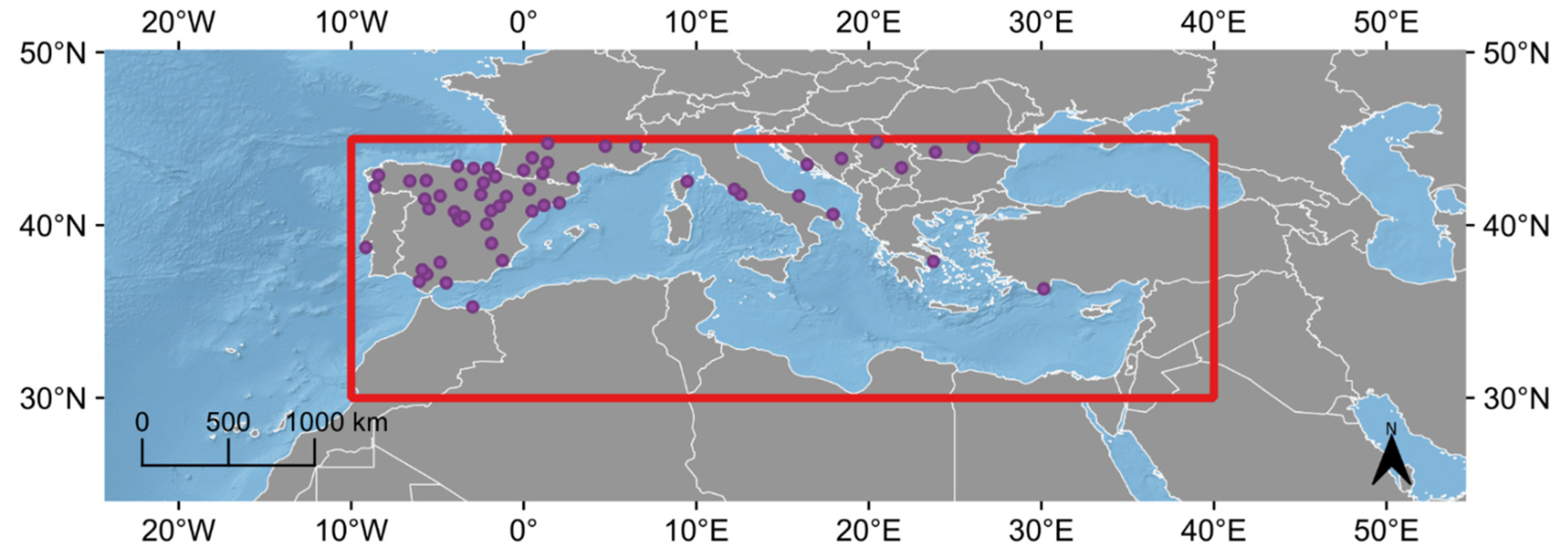
2.1. Weather Station Observations
Daily maximum temperature (Tmax) data (years 1981–2020) were obtained from the Global Historical Climatology Network daily (GHCNd) database, maintained by the National Oceanic and Atmospheric Administration (NOAA) [52]. GHCNd contains daily meteorological measurements from numerous sources (over 80,000 stations worldwide) that have been merged and subjected to common quality control. A subset of the database was used, selecting the stations located within the Mediterranean region (30°N to 45°N, 10°W to 40°E) (red rectangle in Figure 1); the area boundaries used here follow the reference regions of the Sixth Assessment Report (AR6) of the Intergovernmental Panel on Climate Change (IPCC). Stations were further filtered depending on their data completeness throughout the study. Specifically, for the time series of each station, a year was discarded when more than 10% of daily values were missing during the summer season (June to August). Subsequently, stations with less than 25 years in the historical base period (1981–2010) or less than 5 years in the Aqua/MODIS temporal extent period (2002–2020) were excluded from the analysis. To avoid using MODIS pixels with high water fractions, stations close to the shoreline were not included (<1.5 km distance). It was also required that stations did not exhibit major land cover changes during the study period (i.e., from a vegetated type to urban/bare soil or vice versa). The land cover type of the stations was derived using the MODIS Land Cover Type Version 6 product (MCD12Q1) which provides global land cover types at yearly intervals (2001–2020) at a 500-m resolution [53]; the MODIS International Geosphere-Biosphere Programme (IGBP) scheme was selected. 58 GHCNd stations in the Mediterranean region satisfied the above criteria and were included in this study. The spatial distribution of these weather stations can be seen in Figure 1; a full listing of the stations is given in Appendix A (Table A1). The 20-year modal IGBP land cover value was assigned to each station. The majority of the stations were classified as urban (40%); grasslands (17%), croplands (15%), and savannas (12%) were also frequent land cover types in the study area.
Figure 1.
Locations of the 58 weather stations (in purple) from the GHCNd dataset were used in this study.
2.2. Satellite-Based Measurements
The MODIS Terra/Aqua Land Surface Temperature/Emissivity (LST&E) Daily dataset was used (MOD11A1 & MYD11A1 Version 6.1 products). It provides daily (daytime and nighttime) per-pixel LST, which is retrieved using a generalized split-window (GSW) algorithm for the thermal bands 31 and 32 (at 11 and 12 μm) [54]. The coefficients of the GSW depend on the viewing zenith angle, air temperature, and atmospheric column water vapor [55]; detailed retrieval refinements have been introduced for bare soil surfaces since Collection 6 [56]. Version 6.1 products have been further improved by undergoing various calibration changes. Emissivity values for bands 31 and 32 are assumed known and are assigned a priori based on a land cover classification approach [55,57]. Collection 6 MODIS LST has been extensively validated and is considered to provide consistent and highly accurate LST estimates [58,59].
Complete MODIS LST time series were extracted at the corresponding pixels matching the geographic coordinates of the meteorological stations from Section 2.1. Using the quality assurance band of the products, “good data quality” pixel values with estimated emissivity error <= 0.04 and LST error <= 2 K were used. Terra/MODIS dataset was subset temporally to match the coverage of Aqua/MODIS; i.e., the timespan considered in this study for remotely sensed data was from 4 July 2002 to 31 August 2020. The Terra satellite’s daytime overpass time in the Mediterranean region is 09–11 UTC for daytime and 20–22 UTC for nighttime; Aqua has overpass times at about 11–13 UTC and 00–02 UTC.
2.3. Heatwaves
The CTX90pct and CTN90pct heatwave definitions [19] were employed to detect Mediterranean heatwaves from 2002–2020. According to CTX90pct, a heatwave is detected when 3 or more consecutive days are above the climatologic 90th percentile of Tmax; CTN90pct follows the same approach as CTX90pct using Tmin instead. The 90th percentile thresholds are defined independently for each calendar day based on a 15-day moving window (centered on a specific day) of daily Tmax (CTX90pct) and Tmin (CTN90pct) values over the base period 1981–2010 [30]. Each heatwave episode was described by the start date, the duration, and the average daily Tmax (Tmin). Additionally, the following annual heatwave metrics were computed: (i) the annual number of heatwave episodes (HWN), (ii) the sum of heatwave days per year (HWF), and iii) the length (in days) of the longest heatwave per year (HWD) [19]. The normalized heatwave magnitude was computed as the anomaly of the mean Tmax (Tmin) of a given heatwave against the respective summertime mean Tmax or Tmin [19]. Only heatwave events during the summer season (June-August) were included in the analysis.
2.4. LST Anomalies
This paper aims to assess the degree of alignment between heatwaves and LST thermal anomalies. Generally, thermal anomalies reflect a departure of the surface from a baseline condition [31,47]. Here the focus is not only on single (1 day) threshold anomalies but also on anomalies that persist for a number of consecutive days. Thus, LST anomaly events were detected using an approach resembling the heatwave definition in Section 2.3 and similar frameworks used to analyze marine heatwaves (MHWs) [23] or evapotranspiration anomalies [60].
MODIS LST retrievals are affected by the varying satellite overpass time over a given study area—also linked to the sensor viewing angle—; representative examples of this dependence are given in Figure 2. To account for these day-to-day variations, the daily LST observations for each station were initially grouped in non-overlapping quarter-hour intervals (using the corresponding time of the observation band of the products) that were treated independently in all next steps. Then, daily LST anomalies were computed by subtracting a 19-year (2002–2020) nth percentile value, estimated using a 15-day moving window. Several different percentiles (i.e., different LST anomaly indices) were evaluated, ranging from the 65th to the 95th percentile. Using a percentile-based instead of a standard deviation-based threshold has the benefit that no assumption is required regarding the underlying distribution of anomalies [23]. It was considered both the case of single-day LST anomalies and the requirement of a minimum number of consecutive days that the threshold should be exceeded. Given the frequent data gaps in LST time series (e.g., due to clouds or low-quality pixel values), a joint Terra and Aqua approach was also assessed where the daily anomaly threshold could be crossed by either platform. For simplicity, hereafter, we refer to the derived LST anomaly indices simply as LST anomalies.
Figure 2.
Mean daytime MODIS LST (Aqua, MYD11A1) (June–August 2002–2020) as a function of the local overpass time (in UTC) for the locations of GHCNd stations (a) SP000008410 (Cordoba, Spain), (b) IT000016239 (Rome, Italy), and (c) TU000017375 (Finike, Turkey).
Finally, the coincidence rate between LST anomalies and heatwave episodes was derived. Namely, the match percentage between the two datasets was computed, defined as the percent of heatwaves (both as discrete events and as individual days) that were also identified as LST anomalies.
3. Results
To reliably assess which definitions of LST anomalies used in this study show a greater match with heatwave events, they were initially evaluated in terms of their overall systematic differences with heatwaves in climatology. Table 1 shows the average annual sum of heatwave days (HWF) across the area for site-based heatwaves and for the LST anomalies for which the climatology is best captured (the 10 anomalies with the smallest systematic biases). For the anomalies presented in this table and throughout the text, the naming convention followed is: “MxD_Pxx_Dx” where MxD denotes the platform (MOD: Terra; MYD: Aqua; MXD: joint case), Pxx the percentile used, and Dx the required minimum duration of a discrete event in days. As can be seen, anomalies using the joint Terra and Aqua approach (MXD_P85_D3, MXD_P90_D2, and MXD_P95_D1) reproduced with small discrepancies and more consistently for daytime and nighttime the climatology of extreme temperature days in the region. LST anomalies that were derived using only Terra or Aqua did not perform adequately for either daytime or nighttime cases. Interestingly, Aqua, albeit more temporally coincident with daily maximum LSTs, exhibited a weaker performance than Terra. For a few cases, the percentile values for LST anomalies in Table 1 were lower than the 90th percentile of the heatwave definition, which can be largely attributed to the different base periods used for LST anomalies (2002–2020) and heatwaves (1981–2010). Overall, the indices MXD_P85_D3, MXD_P90_D2, and MXD_P95_D1 presented a better and more consistent alignment with heatwaves for the whole region and were used in the following sections of the study. One should note that the values of the proposed percentile thresholds are dependent on the choice of the base period for heatwaves (1981–2010).
Table 1.
Mean annual frequencies (number of days, HWF) of heatwaves (CTX90pct & CTN90pct; in italic font) and LST anomaly days (the 10 best performing indices are shown).
The degree that the identified events align in terms of climatology and trends can further be seen in Figure 3a–d, which presents annual (summer season) metrics (number of events and days) for heatwaves and LST anomalies (MXD_P85_D3). It is evident that the derived LST anomalies largely follow the aggregate climatology of the region with a strong agreement on a year-to-year basis. Notable extremes, such as the 2003 European heatwave, are also well reproduced. Additionally, the average length of the longest event per year (Figure 3e,f) shows coherence between LST and Tair, except for a slight overestimation for MXD_P85_D3 in a few of the years. For both heatwaves and LST anomalies, statistically significant (p < 0.05) rising heatwave metric trends were observed, indicating that extreme hot days are becoming more frequent and persistent. For daytime (nighttime), heatwaves exhibit increasing trends of 1.65 (1.52) days/dec in frequency between 2002 and 2020; LST anomalies increased at a similar rate, 1.35 days/dec for daytime and 1.64 days/dec for nighttime. It is worth noting that the rising trends and the alignment between the two approaches were quite robust regarding the choice of the base period for heatwave detection. As expected, however, the computed values for trends are shaped by the base periods; e.g., computing heatwaves using the reference period 2002–2020, a statistically significant positive trend for HWF of 0.92 (0.75) days/dec for daytime (nighttime) was found.

Figure 3.
Timeseries of HWN (a,b), HWF (c,d), and HWD (e,f) for summer heatwaves (CTX90pct and CTN90pct) and LST anomalies (MXD_P85_D3) in the Mediterranean region (2002–2020); dashed lines represent trends.
In Table 2, the match percentage between heatwaves and LST anomalies (using the three best performing cases of Table 1) is given. The match for events corresponds to the percent of heatwave events that overlapped with an LST anomaly for each location (only shown for LST anomalies with the same minimum duration as heatwaves); for the case of days, the match shows the percent of exact heatwave days that were also identified as LST anomalies. In summary, ≈40% of heatwave days coincided with LST anomaly days during daytime and ≈37% during nighttime; small differences were found among the examined LST anomaly definitions. It was observed that 48% of heatwave episodes co-occurred with an MXD_P85_D3 surface anomaly for at least a single day. Conversely, as presented in Table 3, 48% of days with an LST anomaly overlapped with the exact days of a heatwave during the daytime (38% at night). The similarity of heatwave events that coincided with an LST anomaly was further assessed concerning the heatwave magnitude (Figure 4 and Figure 5). In these figures, the lowess (locally weighted scatterplot smoothing) non-parametric regression [61] was used to determine the best-fitting line. As shown, the match percentage tends to distinctively increase with increasing intensity; when focusing on the more extreme episodes, the match for days presented a notable rise, up to 80% for daytime and 70% for nighttime. Coincidence rates exhibited less variability when examined by the land cover type of the meteorological stations (Figure 6). It was found that land cover did not show as large of an association with MXD_P85_D3 performance; moreover, no systematic bias was observed for the cases of weaker agreement (i.e., open shrublands during daytime and urban during nighttime). It was observed that the choice of the base period for the heatwave detection did not generally affect the results of Table 2 and Table 3 and Figure 4, Figure 5 and Figure 6, as repeating the analysis using the 1961–1990 period (and subsequently different percentiles for the LST anomalies) led to similar findings.
Table 2.
Overall match percentage corresponding to the percent of heatwave events and days that coincide with LST anomalies.
Table 3.
Overall match percentage corresponding to the percent of LST anomalies events and days that coincide with heatwaves.
Figure 4.
Match percentage between heatwave days and LST anomalies as a function of the normalized heatwave magnitude during daytime for (a) MXD_P85_D3, (b) MXD_P90_D2, and (c) MXD_P95_D1; blue curves correspond to the lowess regression lines; error bars correspond to half standard deviation.
Figure 5.
As in Figure 4, during nighttime.
Figure 6.
Match percentage between heatwave days and LST anomalies (MXD_P85_D3) per land cover type for (a) daytime and (b) nighttime. Only land cover types with at least 5% coverage are included.
Next, the match percentage of the exact days identified both as heatwaves and LST anomalies was assessed as a function of the number of days since the start of a given heatwave episode (Figure 7 and Figure 8). As shown, the first days of a heatwave were found to broadly have a weaker agreement with LST anomalies. As the heatwave progresses, the match percentage tends to increase—over 80% and 75% for daytime and nighttime—for long-lasting heatwaves with a duration of over 10 days. Interestingly, daytime LST was found to have generally higher values as heatwave events evolved (Figure 9a and Figure 10a). A much weaker control of the days since the start of an episode on nocturnal LSTs is shown in Figure 9b and Figure 10b. The general associations for match percentage and LST anomalies depicted in Figure 7, Figure 8, Figure 9 and Figure 10 were found to be consistent also for different heatwave base periods (1961–1990).
Figure 7.
Match percentage between heatwave days and LST anomalies as a function of the number of days since the start of an episode during daytime for (a) MXD_P85_D3, (b) MXD_P90_D2, and (c) MXD_P95_D1; blue curves correspond to the lowess regression lines; error bars correspond to half standard deviation.
Figure 8.
As in Figure 7, during nighttime.
Figure 9.
LST anomalies (Terra/MODIS (MOD11A1) (MXD_P85_D3) as a function of the number of days since the start of an episode for (a) daytime (b) nighttime; blue curves correspond to the lowess regression lines; error bars correspond to half standard deviation.
Figure 10.
As in Figure 9, for Aqua/MODIS (MYD11A1).
In Figure 11, LST anomalies (MXD_P85_D3) are shown for selected heatwaves in the Mediterranean. Namely, (a) the 2003 heatwave in Central Europe [1,25] (Figure 11a), (b) the 2006 heatwave in France [62] (Figure 11b), (c) the 2007 heatwave in the Balkans [8,63] (Figure 11c), and (d) the 2019 heatwave in Central Europe [64] (Figure 11d) were included. As can be seen, the LST-based approach of this study presented a strong alignment with station-based heatwave events of these case studies. The necessity of joint use of Terra/Aqua due to discontinuities in LST retrievals is also highlighted. It is worth noting that high LSTs persisted between the two discrete 2007 heatwaves (Figure 11c), potentially influencing the initiation of the second event. Figure 11d shows a representative case where LST progressively increases as the heatwave evolves, shown on aggregate in Figure 9a and Figure 10a.
Figure 11.
LST anomalies during selected heatwaves in the Mediterranean. (a) the 2003 heatwave in Central Europe (FRE00104112; Embrun, France), (b) the 2006 heatwave in France (FRE00104907; Montélimar, France), (c) the 2007 heatwave in the Balkans (ROE00108893; Craiova, Romania), and (d) the 2019 heatwave in Central Europe (SPE00120350; Pamplona, Spain). Shaded areas indicate the dates under a heatwave episode (CTX90pct). The red line corresponds to Terra/MODIS and the purple line to Aqua/MODIS.
4. Conclusions
LST has been widely employed in the literature to describe heatwave episodes; however, relatively little is known about whether anomalously high LST and heatwaves co-occur spatially and temporally. In this paper, it was demonstrated that using the proposed LST index (MXD_P85_D3), during the daytime, on average 42% percent of Mediterranean heatwave days and 47% of heatwave events coincided with LST anomalies (Table 2). Conversely, 51% of daytime LST anomalies days aligned with a heatwave day (Table 3). Nighttime agreement was generally slightly weaker. The observed match percentages are considered relatively high when considering the difference in terms of magnitude, diurnal fluctuation, and response to atmospheric conditions of LST and Tair [27]. For comparison, Sheridan et al. (2020) [65] assessed station and reanalysis-based extreme heat events and found a coincidence rate of 57.5% to 72%, depending on the reanalysis product. Moreover, a stronger co-occurrence was obtained here for the higher intensity heatwave episodes, up to an 80% match percentage (Figure 4 and Figure 5). This agrees with the findings of Mildrexler et al. (2018) [31], where LSTmax anomalies and extreme climatic events were assessed. In future work, a larger number of examined locations across climate types is warranted to evaluate further whether the best performing LST anomalies and the observed coincidence rates are robust. Moreover, while the match percentage was not driven by land cover in the current work, the association of LST during extreme hot days with land cover warrants further investigation in more detail and on a global scale. This may lead to the identification of areas in which heatwave does not severely impact LST; or, conversely, to use LST as an indicator of the heatwave intensity.
It was also observed that the co-occurrence of heatwaves and LST anomalies tends to be significantly higher (up to an 80% match) as the heatwave progresses (Figure 7 and Figure 8). An interpretation of the above relation can be given by considering the physical processes behind the initiation and the evolution of a heatwave. Typically, prevailing synoptic patterns are critical for the occurrence of an extreme event [25]. Given the high atmospheric demand for water during a heatwave, soil desiccation intensifies, surface evaporation progressively drops, and a larger proportion of incoming solar radiation is used to warm up the surface [66]. Moreover, land-atmospheric feedbacks increasingly strengthen; the diurnal convection is intensified, and heat is stored in a deep warm nocturnal residual layer, whereby accumulated heat re-enters the mixed layer in the following days [25]. This land-atmospheric coupling during heatwaves has been previously studied using soil moisture observations [25,66,67,68]; in this work, this LST-Tair coupling was indicated through the progressively higher association between LST anomalies and heatwaves. Daytime LST anomalies tended to increase as the heatwave progresses (Figure 9a and Figure 10a), which may be dictated by soil desiccation and the multi-day heat storage; nevertheless, further investigation is warranted as high uncertainty was observed.
While remotely sensed observations provide spatially exhaustive coverage, MODIS LST spatial resolution may not reflect smaller-scale physical processes that shape the corresponding ground-based air temperature. That is, MODIS footprints (1 km × 1 km) cover a non-homogeneous area, potentially including several land-cover types. Finer scale thermal sensors (e.g., Landsat Thermal Infrared Sensor (TIRS) or ECOSTRESS) cannot provide the repetitive imaging that heatwave episodes require due to their infrequent sampling times. Using a thermal sharpening technique [69] to produce spatially and temporally detailed imagery could improve the alignment between heatwaves and LST anomalies. It is worth noting that the MODIS LST products (MOD11A1 and MYD11A1) used in this study retrieve LST using a classification-based emissivity assignment; this is relatively prone to dynamic errors that may occur after natural surface changes, such as the depletion of soil moisture during a heatwave. The more recent MOD21A1 and MYD21A1 products use the Temperature Emissivity Separation (TES) algorithm, which dynamically retrieves LST and emissivity from three thermal bands [70] and subsequently, in theory, might be better suited for the case of extreme climatic conditions. Nevertheless, it was found that these products had time series with significantly larger discontinuities due to TES convergence issues and hence were not included in the analysis.
In this study, the long-term association between heatwaves and MODIS LST anomalies was examined in the Mediterranean region. A wide range of LST anomaly definitions were evaluated; it was found that the joint Terra and Aqua approach resulted in more consistent indices that can be used both during daytime and nighttime. It was demonstrated that LST anomalies could reproduce the overall climatology of the region and are significantly indicative of heatwaves, especially those of higher intensity. The observed higher coincidence rate as heatwave events evolve reflects the physical processes underlying the more persistent heatwaves (land-atmosphere positive feedback). Overall, results support the case that satellite monitoring can provide important insights in areas with sparse weather-station coverage and assist in heat mitigation strategies.
Author Contributions
I.A., C.C., A.P., T.M. and K.P. designed the methodology. I.A. implemented the methodology and performed the statistical analysis; I.A., C.C., A.P., T.M. and K.P. authors contributed to the analysis of the data, interpretation of the results, and the writing of the paper. All authors have read and agreed to the published version of the manuscript.
Funding
This research was funded by the project “National Network for Climate Change and its Impacts–CLIMPACT”, implemented under the action “National Research Networks Infrastructures in the Fields of Medical Precision, Quantum Technologies and Climate Change” (code no. 2018ΣΕ01300001) financed by the Public Investments Program of Greece.
Data Availability Statement
The GHCNd dataset archive is available from NOAA (https://www.ncei.noaa.gov/data/global-historical-climatology-network-daily/archive/, (accessed on 18 November 2021)). MODIS LST products (MOD11A1 and MYD11A1, V6.1) were accessed from NASA’s Application for Extracting and Exploring Analysis Ready Samples (AρρEEARS) (https://appeears.earthdatacloud.nasa.gov/). The MCD12Q1 V6 IGBP land cover product was accessed through the Google Earth Engine platform (https://code.earthengine.google.com/). The code for reproducing the analysis is provided in a GitHub repository (https://github.com/agathangelidis/heatwaves_lst) (latest version accessed on 18 June 2022).
Conflicts of Interest
The authors declare no conflict of interest.
Appendix A
Table A1.
Full list of the 58 weather stations from the GHCNd dataset used in this study.
Table A1.
Full list of the 58 weather stations from the GHCNd dataset used in this study.
| Code | Name | Country | Lat. | Lon. | Elevation | Land Cover 1 |
|---|---|---|---|---|---|---|
| BKM00014654 | Sarajevo | Bosnia and Herzegovina | 43.868 | 18.423 | 630 | 13 |
| FR000007630 | Toulouse-Blagnac | France | 43.621 | 1.379 | 151 | 10 |
| FR000007747 | Perpignan | France | 42.737 | 2.873 | 42 | 13 |
| FRE00104112 | Embrun | France | 44.566 | 6.502 | 871 | 13 |
| FRE00104116 | Tarbes-Ossun | France | 43.188 | 0 | 360 | 14 |
| FRE00104124 | Bastia | France | 42.541 | 9.485 | 10 | 10 |
| FRE00104907 | Montelimar | France | 44.581 | 4.733 | 73 | 13 |
| FRE00106203 | Mont-De-Marsan | France | 43.909 | 0.500 | 59 | 12 |
| FRE00106205 | St-Girons | France | 43.005 | 1.107 | 414 | 9 |
| FRM00007535 | Gourdon | France | 44.745 | 1.397 | 260 | 9 |
| GR000016716 | Hellinikon | Greece | 37.9 | 23.75 | 10 | 13 |
| HRE00105217 | Split Marjan | Croatia | 43.517 | 16.433 | 122 | 13 |
| IT000016239 | Roma Ciampino | Italy | 41.783 | 12.583 | 105 | 12 |
| IT000016320 | Brindisi | Italy | 40.633 | 17.933 | 10 | 13 |
| IT000162240 | Vigna Di Valle | Italy | 42.083 | 12.217 | 266 | 11 |
| IT000162580 | Monte S. Angelo | Italy | 41.7 | 15.95 | 844 | 10 |
| PO000008535 | Lisboa Geofisica | Portugal | 38.717 | −9.15 | 77 | 13 |
| RIE00100814 | Nis | Serbia | 43.333 | 21.9 | 201 | 13 |
| RIE00100818 | Belgrade (Observatory) | Serbia | 44.8 | 20.467 | 132 | 13 |
| ROE00108889 | Bucuresti-Baneasa | Romania | 44.517 | 26.083 | 90 | 13 |
| ROE00108893 | Craiova | Romania | 44.23 | 23.87 | 192 | 12 |
| SP000003195 | Madrid-Retiro | Spain | 40.412 | −3.678 | 667 | 13 |
| SP000006155 | Malaga Aeropuerto | Spain | 36.667 | −4.488 | 7 | 13 |
| SP000008027 | San Sebastian-Igueldo | Spain | 43.307 | −2.039 | 251 | 8 |
| SP000008181 | Barcelona/Aeropuerto | Spain | 41.293 | 2.0697 | 4 | 13 |
| SP000008202 | Salamanca Aeropuerto | Spain | 40.959 | −5.498 | 790 | 12 |
| SP000008215 | Navacerrada | Spain | 40.781 | −4.01 | 1894 | 9 |
| SP000008280 | Albacete Los Llanos | Spain | 38.952 | −1.863 | 704 | 7 |
| SP000008410 | Cordoba Aeropuerto | Spain | 37.844 | −4.846 | 90 | 9 |
| SP000009434 | Zaragoza Aeropuerto | Spain | 41.662 | −1.008 | 247 | 7 |
| SP000009981 | Tortosa-Observatorio Del Ebr | Spain | 40.821 | 0.491 | 44 | 9 |
| SP000060338 | Melilla | Morocco | 35.278 | −2.955 | 47 | 13 |
| SPE00119729 | Santiago De Compostela/Labacol | Spain | 42.888 | −8.411 | 370 | 8 |
| SPE00119909 | Burgos-Villafria | Spain | 42.356 | −3.632 | 890 | 13 |
| SPE00119945 | Jerez De La Frontera | Spain | 36.751 | −6.056 | 27 | 12 |
| SPE00119990 | Santander/Parayas | Spain | 43.429 | −3.831 | 5 | 13 |
| SPE00120062 | Cuenca | Spain | 40.067 | −2.138 | 945 | 13 |
| SPE00120125 | Molina De Aragon | Spain | 40.844 | −1.885 | 1056 | 7 |
| SPE00120161 | Huesca | Spain | 42.083 | 0.326 | 541 | 10 |
| SPE00120188 | Logrono-Agoncillo | Spain | 42.452 | −2.331 | 353 | 12 |
| SPE00120224 | Leon Virgen Del Camino | Spain | 42.589 | −5.649 | 916 | 10 |
| SPE00120233 | Ponferrada | Spain | 42.564 | −6.6 | 534 | 9 |
| SPE00120278 | Madrid/Barajas | Spain | 40.467 | −3.556 | 609 | 10 |
| SPE00120287 | Madrid/Cuatrovientos | Spain | 40.378 | −3.789 | 687 | 13 |
| SPE00120296 | Madrid/Getafe | Spain | 40.3 | −3.722 | 617 | 13 |
| SPE00120305 | Madrid/Torrejon | Spain | 40.483 | −3.450 | 611 | 7 |
| SPE00120332 | Murcia/Alcantarilla | Spain | 37.958 | −1.229 | 85 | 10 |
| SPE00120350 | Pamplona (Observatorio) | Spain | 42.817 | −1.636 | 442 | 13 |
| SPE00120413 | Vigo Peinador | Spain | 42.239 | −8.624 | 261 | 9 |
| SPE00120503 | Moron De La Frontera | Spain | 37.158 | −5.616 | 87 | 12 |
| SPE00120512 | Sevilla/San Pablo | Spain | 37.417 | −5.879 | 34 | 7 |
| SPE00120521 | Soria | Spain | 41.775 | −2.483 | 1082 | 10 |
| SPE00120530 | Reus/Aeropuerto | Spain | 41.149 | 1.179 | 71 | 10 |
| SPE00120602 | Valladolid (Villanubla) | Spain | 41.7 | −4.85 | 846 | 12 |
| SPE00120611 | Bilbao Aeropuerto | Spain | 43.298 | −2.906 | 42 | 13 |
| SPE00120620 | Zamora | Spain | 41.517 | −5.733 | 656 | 13 |
| SPE00120629 | Daroca | Spain | 41.114 | −1.41 | 779 | 10 |
| TU000017375 | Finike | Turkey | 36.316 | 30.15 | 2 | 12 |
1 7: Open shrublands; 8: Woody savannas; 9: Savannas; 10: Grasslands; 11: Permanent wetlands; 12: Croplands; 13: Urban and built-up; 14: Cropland/natural vegetation mosaic (MODIS IGBP classification scheme).
References
- Fischer, E.M.; Seneviratne, S.I.; Vidale, P.L.; Lüthi, D.; Schär, C. Soil Moisture–Atmosphere Interactions during the 2003 European Summer Heat Wave. J. Clim. 2007, 20, 5081–5099. [Google Scholar] [CrossRef]
- Dole, R.; Hoerling, M.; Perlwitz, J.; Eischeid, J.; Pegion, P.; Zhang, T.; Quan, X.-W.; Xu, T.; Murray, D. Was There a Basis for Anticipating the 2010 Russian Heat Wave? Geophys. Res. Lett. 2011, 38. [Google Scholar] [CrossRef] [Green Version]
- Overland, J.E. Causes of the Record-Breaking Pacific Northwest Heatwave, Late June 2021. Atmosphere 2021, 12, 1434. [Google Scholar] [CrossRef]
- Barriopedro, D.; Fischer, E.M.; Luterbacher, J.; Trigo, R.M.; García-Herrera, R. The Hot Summer of 2010: Redrawing the Temperature Record Map of Europe. Science 2011, 332, 220–224. [Google Scholar] [CrossRef] [PubMed] [Green Version]
- Fischer, E.M.; Sippel, S.; Knutti, R. Increasing Probability of Record-Shattering Climate Extremes. Nat. Clim. Chang. 2021, 11, 689–695. [Google Scholar] [CrossRef]
- Coumou, D.; Rahmstorf, S. A Decade of Weather Extremes. Nat. Clim. Chang. 2012, 2, 491–496. [Google Scholar] [CrossRef]
- Dosio, A.; Mentaschi, L.; Fischer, E.M.; Wyser, K. Extreme Heat Waves under 1.5 °C and 2 °C Global Warming. Environ. Res. Lett. 2018, 13, 054006. [Google Scholar] [CrossRef] [Green Version]
- Russo, S.; Sillmann, J.; Fischer, E.M. Top Ten European Heatwaves since 1950 and Their Occurrence in the Coming Decades. Environ. Res. Lett. 2015, 10, 124003. [Google Scholar] [CrossRef]
- Anderson, G.B.; Bell, M.L. Heat Waves in the United States: Mortality Risk during Heat Waves and Effect Modification by Heat Wave Characteristics in 43 US Communities. Environ. Health Perspect. 2011, 119, 210–218. [Google Scholar] [CrossRef] [Green Version]
- Koppe, C.; Kovats, S.; Jendritzky, G.; Menne, B. Heat-Waves: Risks and Responses; World Health Organization, Regional Office for Europe: Geneva, Switzerland, 2004. [Google Scholar]
- Mora, C.; Counsell, C.W.; Bielecki, C.R.; Louis, L.V. Twenty-Seven Ways a Heat Wave Can Kill You: Deadly Heat in the Era of Climate Change. Circ. Cardiovasc. Qual. Outcomes 2017, 10, e004233. [Google Scholar] [CrossRef]
- Gampe, D.; Zscheischler, J.; Reichstein, M.; O’Sullivan, M.; Smith, W.K.; Sitch, S.; Buermann, W. Increasing Impact of Warm Droughts on Northern Ecosystem Productivity over Recent Decades. Nat. Clim. Chang. 2021, 11, 772–779. [Google Scholar] [CrossRef]
- Stillman, J.H. Heat Waves, the New Normal: Summertime Temperature Extremes Will Impact Animals, Ecosystems, and Human Communities. Physiology 2019, 34, 86–100. [Google Scholar] [CrossRef] [PubMed]
- Burillo, D.; Chester, M.V.; Ruddell, B.; Johnson, N. Electricity Demand Planning Forecasts Should Consider Climate Non-Stationarity to Maintain Reserve Margins during Heat Waves. Appl. Energy 2017, 206, 267–277. [Google Scholar] [CrossRef]
- Alexander, L.V.; Zhang, X.; Peterson, T.C.; Caesar, J.; Gleason, B.; Klein Tank, A.M.G.; Haylock, M.; Collins, D.; Trewin, B.; Rahimzadeh, F.; et al. Global Observed Changes in Daily Climate Extremes of Temperature and Precipitation. J. Geophys. Res. Atmos. 2006, 111, 1042–1063. [Google Scholar] [CrossRef] [Green Version]
- Collins, D.; Della-Marta, P.; Plummer, N.; Trewin, B. Trends in Annual Frequencies of Extreme Temperature Events in Australia. Aust. Meteorol. Mag. 2000, 49, 277–292. [Google Scholar]
- Fischer, E.M.; Schär, C. Consistent Geographical Patterns of Changes in High-Impact European Heatwaves. Nat. Geosci. 2010, 3, 398–403. [Google Scholar] [CrossRef]
- Nairn, J.R.; Fawcett, R.J.B. The Excess Heat Factor: A Metric for Heatwave Intensity and Its Use in Classifying Heatwave Severity. Int. J. Environ. Res. Public. Health 2015, 12, 227–253. [Google Scholar] [CrossRef] [Green Version]
- Perkins, S.E.; Alexander, L.V. On the Measurement of Heat Waves. J. Clim. 2013, 26, 4500–4517. [Google Scholar] [CrossRef]
- Robinson, P.J. On the Definition of a Heat Wave. J. Appl. Meteorol. Climatol. 2001, 40, 762–775. [Google Scholar] [CrossRef]
- Russo, S.; Dosio, A.; Graversen, R.G.; Sillmann, J.; Carrao, H.; Dunbar, M.B.; Singleton, A.; Montagna, P.; Barbola, P.; Vogt, J.V. Magnitude of Extreme Heat Waves in Present Climate and Their Projection in a Warming World. J. Geophys. Res. Atmos. 2014, 119, 12500–12512. [Google Scholar] [CrossRef] [Green Version]
- Perkins, S.E.; Alexander, L.V.; Nairn, J.R. Increasing Frequency, Intensity and Duration of Observed Global Heatwaves and Warm Spells. Geophys. Res. Lett. 2012, 39, 10. [Google Scholar] [CrossRef]
- Hobday, A.J.; Alexander, L.V.; Perkins, S.E.; Smale, D.A.; Straub, S.C.; Oliver, E.C.J.; Benthuysen, J.A.; Burrows, M.T.; Donat, M.G.; Feng, M.; et al. A Hierarchical Approach to Defining Marine Heatwaves. Prog. Oceanogr. 2016, 141, 227–238. [Google Scholar] [CrossRef] [Green Version]
- Perkins, S.E. A Review on the Scientific Understanding of Heatwaves—Their Measurement, Driving Mechanisms, and Changes at the Global Scale. Atmos. Res. 2015, 164–165, 242–267. [Google Scholar] [CrossRef]
- Miralles, D.G.; Teuling, A.J.; van Heerwaarden, C.C.; Vilà-Guerau de Arellano, J. Mega-Heatwave Temperatures Due to Combined Soil Desiccation and Atmospheric Heat Accumulation. Nat. Geosci. 2014, 7, 345–349. [Google Scholar] [CrossRef]
- Zschenderlein, P.; Fink, A.H.; Pfahl, S.; Wernli, H. Processes Determining Heat Waves across Different European Climates. Q. J. R. Meteorol. Soc. 2019, 145, 2973–2989. [Google Scholar] [CrossRef] [Green Version]
- Jin, M.; Dickinson, R.E. Land Surface Skin Temperature Climatology: Benefitting from the Strengths of Satellite Observations. Environ. Res. Lett. 2010, 5, 044004. [Google Scholar] [CrossRef] [Green Version]
- Ceccherini, G.; Russo, S.; Ameztoy, I.; Marchese, A.F.; Carmona-Moreno, C. Heat Waves in Africa 1981–2015, Observations and Reanalysis. Nat. Hazards Earth Syst. Sci. 2017, 17, 115–125. [Google Scholar] [CrossRef] [Green Version]
- Engdaw, M.M.; Ballinger, A.P.; Hegerl, G.C.; Steiner, A.K. Changes in Temperature and Heat Waves over Africa Using Observational and Reanalysis Data Sets. Int. J. Climatol. 2022, 42, 1165–1180. [Google Scholar] [CrossRef]
- Perkins-Kirkpatrick, S.; Lewis, S. Increasing Trends in Regional Heatwaves. Nat. Commun. 2020, 11, 1–8. [Google Scholar] [CrossRef]
- Mildrexler, D.J.; Zhao, M.; Cohen, W.B.; Running, S.W.; Song, X.P.; Jones, M.O. Thermal Anomalies Detect Critical Global Land Surface Changes. J. Appl. Meteorol. Climatol. 2018, 57, 391–411. [Google Scholar] [CrossRef]
- Becker, F.; Li, Z.-L. Surface Temperature and Emissivity at Various Scales: Definition, Measurement and Related Problems. Remote Sens. Rev. 1995, 12, 225–253. [Google Scholar] [CrossRef]
- Norman, J.M.; Becker, F. Terminology in Thermal Infrared Remote Sensing of Natural Surfaces. Agric. For. Meteorol. 1995, 77, 153–166. [Google Scholar] [CrossRef]
- Hulley, G.; Ghent, D. Taking the Temperature of the Earth: Steps towards Integrated Understanding of Variability and Change; Elsevier: Amsterdam, The Netherlands, 2019. [Google Scholar]
- Kuenzer, C.; Dech, S. (Eds.) Thermal Infrared Remote Sensing: Sensors, Methods, Applications; Remote Sensing and Digital Image Processing; Springer: Dordrecht, The Netherlands, 2013; ISBN 978-94-007-6638-9. [Google Scholar]
- Li, Z.-L.; Tang, B.-H.; Wu, H.; Ren, H.; Yan, G.; Wan, Z.; Trigo, I.F.; Sobrino, J.A. Satellite-Derived Land Surface Temperature: Current Status and Perspectives. Remote Sens. Environ. 2013, 131, 14–37. [Google Scholar] [CrossRef] [Green Version]
- Oyler, J.W.; Dobrowski, S.Z.; Holden, Z.A.; Running, S.W. Remotely Sensed Land Skin Temperature as a Spatial Predictor of Air Temperature across the Conterminous United States. J. Appl. Meteorol. Climatol. 2016, 55, 1441–1457. [Google Scholar] [CrossRef]
- Mildrexler, D.J.; Zhao, M.; Running, S.W. A Global Comparison between Station Air Temperatures and MODIS Land Surface Temperatures Reveals the Cooling Role of Forests. J. Geophys. Res. Biogeosci. 2011, 116. [Google Scholar] [CrossRef]
- Cheval, S.; Dumitrescu, A.; Bell, A. The Urban Heat Island of Bucharest during the Extreme High Temperatures of July 2007. Theor. Appl. Climatol. 2009, 97, 391–401. [Google Scholar] [CrossRef]
- Cotlier, G.I.; Jimenez, J.C. The Extreme Heat Wave over Western North America in 2021: An Assessment by Means of Land Surface Temperature. Remote Sens. 2022, 14, 561. [Google Scholar] [CrossRef]
- Dousset, B.; Gourmelon, F.; Laaidi, K.; Zeghnoun, A.; Giraudet, E.; Bretin, P.; Mauri, E.; Vandentorren, S. Satellite Monitoring of Summer Heat Waves in the Paris Metropolitan Area. Int. J. Climatol. 2011, 31, 313–323. [Google Scholar] [CrossRef]
- Hulley, G.; Shivers, S.; Wetherley, E.; Cudd, R. New ECOSTRESS and MODIS Land Surface Temperature Data Reveal Fine-Scale Heat Vulnerability in Cities: A Case Study for Los Angeles County, California. Remote Sens. 2019, 11, 2136. [Google Scholar] [CrossRef] [Green Version]
- Kumar, R.; Mishra, V. Decline in Surface Urban Heat Island Intensity in India during Heatwaves. Environ. Res. Commun. 2019, 1, 031001. [Google Scholar] [CrossRef] [Green Version]
- Ossola, A.; Jenerette, G.D.; McGrath, A.; Chow, W.; Hughes, L.; Leishman, M.R. Small Vegetated Patches Greatly Reduce Urban Surface Temperature during a Summer Heatwave in Adelaide, Australia. Landsc. Urban Plan. 2021, 209, 104046. [Google Scholar] [CrossRef]
- Retalis, A.; Paronis, D.; Lagouvardos, K.; Kotroni, V. The Heat Wave of June 2007 in Athens, Greece—Part 1: Study of Satellite Derived Land Surface Temperature. Atmos. Res. 2010, 98, 458–467. [Google Scholar] [CrossRef]
- Ward, K.; Lauf, S.; Kleinschmit, B.; Endlicher, W. Heat Waves and Urban Heat Islands in Europe: A Review of Relevant Drivers. Sci. Total Environ. 2016, 569–570, 527–539. [Google Scholar] [CrossRef] [PubMed]
- Albright, T.P.; Pidgeon, A.M.; Rittenhouse, C.D.; Clayton, M.K.; Flather, C.H.; Culbert, P.D.; Radeloff, V.C. Heat Waves Measured with MODIS Land Surface Temperature Data Predict Changes in Avian Community Structure. Remote Sens. Environ. 2011, 115, 245–254. [Google Scholar] [CrossRef] [Green Version]
- Baldi, M.; Dalu, G.; Maracchi, G.; Pasqui, M.; Cesarone, F. Heat Waves in the Mediterranean: A Local Feature or a Larger-Scale Effect? Int. J. Climatol. J. R. Meteorol. Soc. 2006, 26, 1477–1487. [Google Scholar] [CrossRef] [Green Version]
- Lionello, P. The Climate of the Mediterranean Region: From the Past to the Future; Elsevier: Amsterdam, The Netherlands, 2012. [Google Scholar]
- Giorgi, F.; Lionello, P. Climate Change Projections for the Mediterranean Region. Glob. Planet. Chang. 2008, 63, 90–104. [Google Scholar] [CrossRef]
- Molina, M.O.; Sánchez, E.; Gutiérrez, C. Future Heat Waves over the Mediterranean from an Euro-CORDEX Regional Climate Model Ensemble. Sci. Rep. 2020, 10, 8801. [Google Scholar] [CrossRef]
- Menne, M.J.; Durre, I.; Vose, R.S.; Gleason, B.E.; Houston, T.G. An Overview of the Global Historical Climatology Network-Daily Database. J. Atmos. Ocean. Technol. 2012, 29, 897–910. [Google Scholar] [CrossRef]
- Sulla-Menashe, D.; Gray, J.M.; Abercrombie, S.P.; Friedl, M.A. Hierarchical Mapping of Annual Global Land Cover 2001 to Present: The MODIS Collection 6 Land Cover Product. Remote Sens. Environ. 2019, 222, 183–194. [Google Scholar] [CrossRef]
- Wan, Z.; Dozier, J. A Generalized Split-Window Algorithm for Retrieving Land-Surface Temperature from Space. IEEE Trans. Geosci. Remote Sens. 1996, 34, 892–905. [Google Scholar]
- Wan, Z. New Refinements and Validation of the MODIS Land-Surface Temperature/Emissivity Products. Remote Sens. Environ. 2008, 112, 59–74. [Google Scholar] [CrossRef]
- Wan, Z. New Refinements and Validation of the Collection-6 MODIS Land-Surface Temperature/Emissivity Product. Remote Sens. Environ. 2014, 140, 36–45. [Google Scholar] [CrossRef]
- Snyder, W.C.; Wan, Z.; Zhang, Y.; Feng, Y.-Z. Classification-Based Emissivity for Land Surface Temperature Measurement from Space. Int. J. Remote Sens. 1998, 19, 2753–2774. [Google Scholar] [CrossRef]
- Duan, S.-B.; Li, Z.-L.; Wu, H.; Leng, P.; Gao, M.; Wang, C. Radiance-Based Validation of Land Surface Temperature Products Derived from Collection 6 MODIS Thermal Infrared Data. Int. J. Appl. Earth Obs. Geoinf. 2018, 70, 84–92. [Google Scholar] [CrossRef]
- Duan, S.-B.; Li, Z.-L.; Li, H.; Göttsche, F.-M.; Wu, H.; Zhao, W.; Leng, P.; Zhang, X.; Coll, C. Validation of Collection 6 MODIS Land Surface Temperature Product Using in Situ Measurements. Remote Sens. Environ. 2019, 225, 16–29. [Google Scholar] [CrossRef] [Green Version]
- Zscheischler, J.; Orth, R.; Seneviratne, S.I. A Submonthly Database for Detecting Changes in Vegetation-Atmosphere Coupling. Geophys. Res. Lett. 2015, 42, 9816–9824. [Google Scholar] [CrossRef] [Green Version]
- Cleveland, W.S. Robust Locally Weighted Regression and Smoothing Scatterplots. J. Am. Stat. Assoc. 1979, 74, 829–836. [Google Scholar] [CrossRef]
- Fouillet, A.; Rey, G.; Wagner, V.; Laaidi, K.; Empereur-Bissonnet, P.; Le Tertre, A.; Frayssinet, P.; Bessemoulin, P.; Laurent, F.; De Crouy-Chanel, P.; et al. Has the Impact of Heat Waves on Mortality Changed in France since the European Heat Wave of Summer 2003? A Study of the 2006 Heat Wave. Int. J. Epidemiol. 2008, 37, 309–317. [Google Scholar] [CrossRef]
- Founda, D.; Giannakopoulos, C. The Exceptionally Hot Summer of 2007 in Athens, Greece—A Typical Summer in the Future Climate? Glob. Planet. Chang. 2009, 67, 227–236. [Google Scholar] [CrossRef]
- Xu, P.; Wang, L.; Liu, Y.; Chen, W.; Huang, P. The Record-Breaking Heat Wave of June 2019 in Central Europe. Atmos. Sci. Lett. 2020, 21, e964. [Google Scholar] [CrossRef] [Green Version]
- Sheridan, S.C.; Lee, C.C.; Smith, E.T. A Comparison Between Station Observations and Reanalysis Data in the Identification of Extreme Temperature Events. Geophys. Res. Lett. 2020, 47, e2020GL088120. [Google Scholar] [CrossRef]
- Fischer, E.M.; Seneviratne, S.I.; Lüthi, D.; Schär, C. Contribution of Land-Atmosphere Coupling to Recent European Summer Heat Waves. Geophys. Res. Lett. 2007, 34. [Google Scholar] [CrossRef] [Green Version]
- Miralles, D.G.; Gentine, P.; Seneviratne, S.I.; Teuling, A.J. Land–Atmospheric Feedbacks during Droughts and Heatwaves: State of the Science and Current Challenges. Ann. N. Y. Acad. Sci. 2019, 1436, 19–35. [Google Scholar] [CrossRef] [PubMed]
- Geirinhas, J.L.; Russo, A.C.; Libonati, R.; Miralles, D.G.; Sousa, P.M.; Wouters, H.; Trigo, R.M. The Influence of Soil Dry-out on the Record-Breaking Hot 2013/2014 Summer in Southeast Brazil. Sci. Rep. 2022, 12, 5836. [Google Scholar] [CrossRef]
- Zhan, W.; Chen, Y.; Zhou, J.; Wang, J.; Liu, W.; Voogt, J.; Zhu, X.; Quan, J.; Li, J. Disaggregation of Remotely Sensed Land Surface Temperature: Literature Survey, Taxonomy, Issues, and Caveats. Remote Sens. Environ. 2013, 131, 119–139. [Google Scholar] [CrossRef]
- Malakar, N.K.; Hulley, G.C. A Water Vapor Scaling Model for Improved Land Surface Temperature and Emissivity Separation of MODIS Thermal Infrared Data. Remote Sens. Environ. 2016, 182, 252–264. [Google Scholar] [CrossRef]
Publisher’s Note: MDPI stays neutral with regard to jurisdictional claims in published maps and institutional affiliations. |
© 2022 by the authors. Licensee MDPI, Basel, Switzerland. This article is an open access article distributed under the terms and conditions of the Creative Commons Attribution (CC BY) license (https://creativecommons.org/licenses/by/4.0/).