RSSGG_CS: Remote Sensing Image Scene Graph Generation by Fusing Contextual Information and Statistical Knowledge

Abstract

To semantically understand remote sensing images, it is not only necessary to detect the objects in them but also to recognize the semantic relationships between the instances. Scene graph generation aims to represent the image as a semantic structural graph, where objects and relationships between them are described as nodes and edges, respectively. Some existing methods rely only on visual features to sequentially predict the relationships between objects, ignoring contextual information and making it difficult to generate high-quality scene graphs, especially for remote sensing images. Therefore, we propose a novel model for remote sensing image scene graph generation by fusing contextual information and statistical knowledge, namely RSSGG_CS. To integrate contextual information and calculate attention among all objects, the RSSGG_CS model adopts a filter module (FiM) that is based on adjusted transformer architecture. Moreover, to reduce the blindness of the model when searching semantic space, statistical knowledge of relational predicates between objects from the training dataset and the cleaned Wikipedia text is used as supervision when training the model. Experiments show that fusing contextual information and statistical knowledge allows the model to generate more complete scene graphs of remote sensing images and facilitates the semantic understanding of remote sensing images.

1. Introduction

1.1. Background of Scene Graph Generation

Deep learning methods based on data-driven methods have significantly promoted the development of computer vision. Existing methods already have superior performance for some tasks performed on individual instances, such as object detection [1,2] and instance segmentation [3,4]. These methods distinguish independent objects from the image background but do not explore the semantic relationships between objects [5]. Objects in an image constitute the overall content, but the semantic relationships between instances determine how the image gist is interpreted [6]. Hence, more and more research has focused on extracting the semantic relationships between instances. Scene graph generation localizes not only objects but also recognizes their relationships, which is a visual task with higher semantic abstraction. As a structural representation of images, the objects and their semantic relationships are represented as nodes and edges in the scene graph [5,7,8,9]. There are a series of triples, <subject-predicate-object>, in the scene graph, “predicate” represents a specific semantic relationship, and “subject” and “object” are the two instances involved, as shown in Figure 1c. As a bridge between low-level recognition and high-level understanding of images, the scene graph supports many downstream vision tasks [8,9,10,11,12], such as image captioning [13,14] and visual question answering [15,16].

1.1.1. Classical Methods for Scene Graph Generation

Scene graph generation is one of the computer vision tasks used to understand images abstractly, which localizes the objects and recognizes their relationships [7]. Ref. [17] constructed the large-scale Visual Genome dataset, which significantly promoted the research on scene graph generation. However, there are some tricky problems in the dataset, such as the long tail problem [10,18,19] and inconsistent labeling of similar semantic relationships [20,21]. Ref. [6] leveraged language priors into the visual relationship detection and tried to improve the model performance with non-visual content. In some methods, object detection and relationship predicate prediction are often divided into two processes [5,8]. The model structure of these methods is separated into two parts. Ref. [22] simultaneously detected object pairs and predicted the potential relationships on the image feature maps to generate the scene graph in a unified network. Fusing contextual features is necessary for generating high-quality scene graphs. Ref. [23] showed that global hints have strong influences in predicting relations and proposed the HCNet to integrate different levels of information. IMP improved the model’s performance for scene graph generation by passing contextual information [24].

Gradually, some researchers have found that it is impossible to fully understand the meaning of the image only by relying on the image content itself, and it is crucial to introduce external knowledge to understand the image semantically [19,25]. VCTree explored the structural information of instances in images to enhance the semantic understanding of image contents [26]. MOTIFS pointed out that the semantic labels of objects alone can predict many relationships for object pairs [27]. The introduction of external knowledge in existing scene graph generation methods can be divided into two categories: (1) using external knowledge to enhance the features of objects; (2) optimizing the model as supervision. Ref. [10] retrieved the facts from ConceptNet and then mixed them with the objects detected from images to enhance the visual representation of images. Refs. [19,28] used internal and external knowledge distillation to regularize the model learning. Knowledge graphs were bridged to generate scene graphs in [25], and the scene graph generation was regarded as the bridge between the scene and commonsense graphs. The image captions were treated as the image gist knowledge to generate topic scene graphs [29]. Introducing richer knowledge will make the generated scene graphs more flexible and diverse.

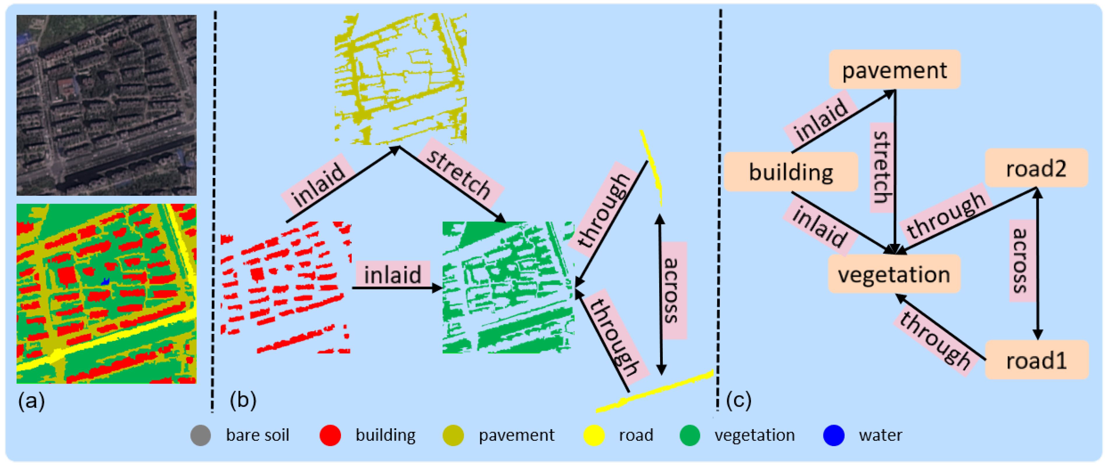
1.1.2. High-Level Understanding of Remote Sensing Image

There have been many studies on scene graph generation for natural scene images, but few studies focus on understanding remote sensing images semantically, and even fewer focus on remote sensing image scene graph generation. In some sub-fields of computer vision, the characteristics of remote sensing images make some methods with good performance in natural scenes perform poorly on remote sensing images and often require targeted improvements. For example, in the research of image dehazing, both [30,31] have designed proprietary models for the characteristics of remote sensing images to make the processed images have better visual effects. In the research of scene graph generation for remote sensing images, it is essential to design datasets and models for their characteristics to understand them semantically. MSRIN [32] was proposed as a parallel deep neural network to recognize the objects and their spatial relationships in remote sensing images. However, MSRIN does not present these spatial relationships semantically and intuitively. Ref. [33] carried out research on remote sensing image scene graph generation and proposed a related dataset RSSGD. Although this research has inspired the semantic understanding of remote sensing images, it lacked consideration of the characteristics of remote sensing images. The SRSG model pointed out that the relationships between objects in remote sensing images are more dependent on their morphological features and took the segmentation results as input directly. The study of semantically understanding remote sensing images is greatly promoted by these studies. However, the further development of remote sensing image scene graph generation is limited by the abstraction ability of object features and the lack of commonsense knowledge.

1.2. Challenges of Scene Graph Generation

Abstracting the semantic relationship in remote sensing images is also essential to understanding their meanings. However, some common problems of scene graph generation and the lack of related research have plagued the semantic understanding of remote sensing images. There are two typical problems in scene graph generation: (1) it is challenging to integrate the entire image content when detecting semantic relationships; (2) the image content alone is not enough for a deep understanding of the image [19]. Some early methods detect visual relationships between objects one by one without considering the connections of these relationships from the perspective of the whole image [6], which cannot describe the structure of the entire scene [5]. The surrounding objects are beneficial for detecting the visual relationship of the current object pair. Therefore, fusing contextual features to specific object pairs is the key to integrating the complete scene information. Fusing local and global features is incredibly beneficial to fully understand image information, as is the case in many computer vision research, such as image dehazing [34], object detection [35], and so on. Common sense knowledge facilitates visual comprehension when humans observe an image. That is to say, the abstract semantic reasoning process is difficult to present by itself in the image pixel set [25]. It is not easy to measure how much our own prior knowledge and the inherent content of the image play a role in understanding the image, respectively. However, one thing is sure: the image can be interpreted from a higher semantic level by importing external knowledge. In addition to the problems mentioned above, the characteristics of remote sensing images themselves also make it more challenging to generate scene graphs. Since remote sensing images are obtained from an overhead view, the objects are distributed in the whole scene, and most things are highly chaotic, such as Figure 1a, unlike natural images where objects are mainly distributed at the scene’s bottom. At present, few studies and datasets focus on exploring the semantic relationship of objects in remote sensing images. These difficulties make it more challenging to extract the semantic relationships between objects in remote sensing images.

1.3. Contributions of the Paper

In this paper, we propose a novel remote sensing image scene graph generation model, RSSGG_CS, by fusing contextual information and statistical knowledge, as shown in Figure 2. When predicting the semantic relationships between object pairs, only using local features of the subject and object will make the relationship search space too large; the model needs to explore all candidates for suitable relationship predicates. However, the entire image content provides contextual information and a powerful constraint for predicting the relationship of specific instance pairs [22]. Therefore, to incorporate the contextual information for all instances in the current image, a filter module (FiM) based on an adjusted transformer [36] architecture is adopted in RSSGG_CS. In this way, the features of each object are enhanced, and the weight among instances can be calculated; thereby, the object pairs without semantic relationships are suppressed, and the search space of relationship predicates is greatly reduced.

The semantic relationships between entities in the real world conform to a specific distribution; for example, in most cases, the relationship between river and vegetation is <river-through-vegetation>. The distribution of relationships among some specific instances is inherently independent of the dataset. Moreover, as the sub-space of the real world, the distribution of relationships between objects in datasets should be consistent with the real world. Statistical knowledge about object relationships extracted from the dataset and the people’s daily actual data is a critical supplement for predicting relationship predicates [37]. Therefore, the distribution of relationships among instances can be introduced into the model as statistical knowledge. In the RSSGG_CS model, we introduce this statistical knowledge from two sources: (1) the training dataset and (2) the cleaned Wikipedia text. In this way, as the training progresses, the distribution of the model output gradually approaches the distribution of statistical knowledge, and the blindness of the prediction is reduced dramatically. Thus the model will also be able to predict relationships between instances more accurately.

Furthermore, the objects in remote sensing images are highly mixed, and their relationships are more dependent on their morphological features. The segmentation results of each object encode its morphological features; the visual features and category semantic embeddings directly contain high-level semantic information. Therefore, in the RSSGG_CS model, we combine all objects’ visual features with their category of semantic embeddings together to supplement the remote sensing image segmentation results. The process of visual feature extraction is simplified by importing such high-level semantic information [38].

In this paper, we propose a model, RSSGG_CS, for remote sensing image scene graph generation and enhance the performance of the model by fusing statistical knowledge and contextual information. Our contributions are as follows:

• We propose a novel model, RSSGG_CS, for remote sensing image scene graph generation;
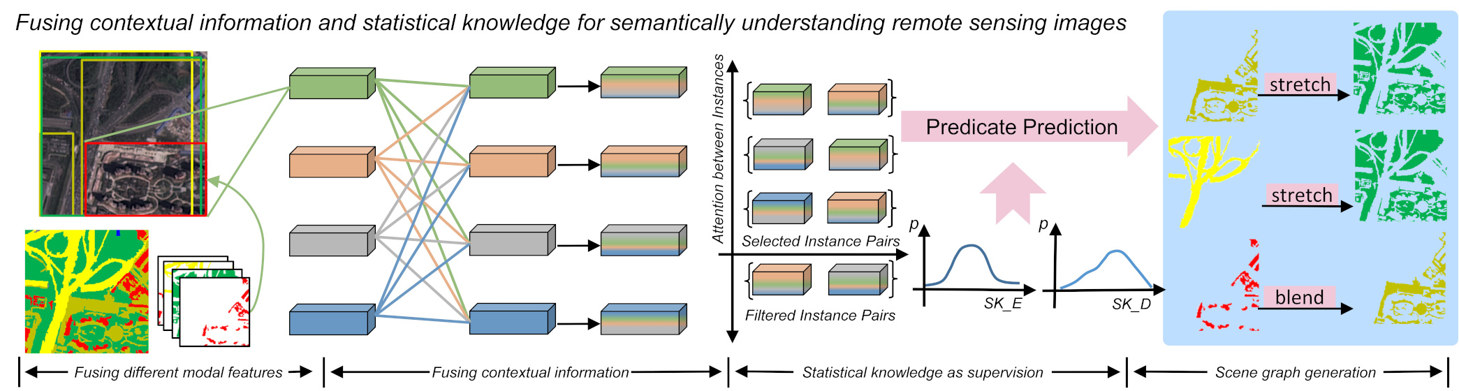
• We fuse contextual information for each object by the FiM to enhance the feature extraction ability of the model and suppress object pairs without semantic relationships when generating remote sensing image scene graphs;
• We import statistical knowledge for the RSSGG_CS model to reduce the blindness of predicting the relationships between objects in remote sensing images;
• We combine the visual features and category semantic embeddings of objects to enhance the semantic expressiveness of the RSSGG_CS model.

2. Materials and Methods

In this section, the structure and implementation of the RSSGG_CS model are presented in detail.

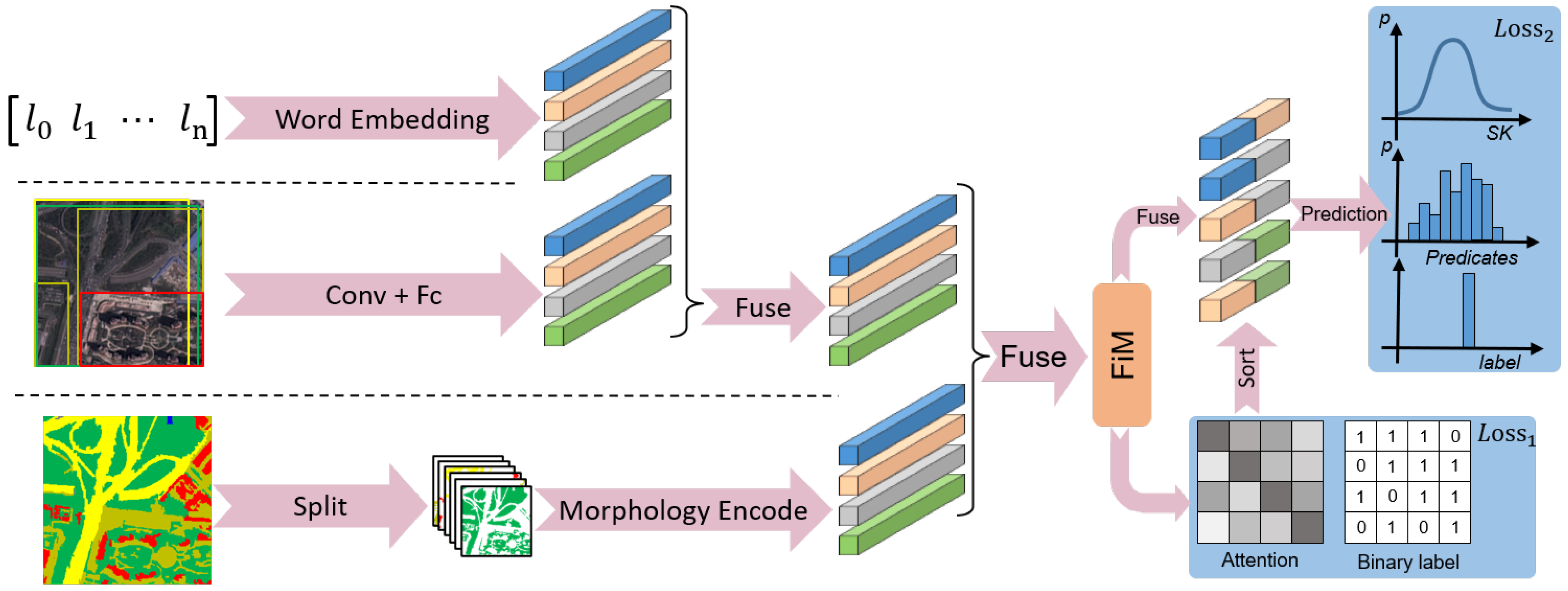
2.1. The Structure of RSSGG_CS

The RSSGG_CS model is combined with three parallel feature extraction branches and the FiM module, as shown in Figure 2. The three parallel feature extraction branches are the object category semantic embedding branch, the visual feature extraction branch, and the segmentation result morphological feature encoding branch. Various features of remote sensing images are separated from different dimensions by the three branches and then connected and input into the FiM module. The FiM model is a transformer-based attention computation unit. Features of the pairwise instances are fused in the FiM module, and the attention between instances is also calculated in it. The degree of correlation between instances is reflected by the attention, which indicates whether there is an actual semantic relationship between the two objects. To make the model converge quickly, the output of the FiM final layer will be added to the loss function to suppress the excessive attention between unrelated instances. Then the object features will be sorted and combined according to their correlation and input fully connected layer to predict relationship predicates.

To integrate statistical knowledge into the RSSGG_CS model, we incorporate statistical knowledge into the loss function to complement the supervision. Therefore, the annotation information, the statistical knowledge of the dataset, and commonsense knowledge should be considered in the supervision when calculating the loss of the model. In this way, the total loss of RSSGG_CS will include the attention loss of the FiM output and the final prediction loss. Next, we will describe each component of the RSSGG_CS model in detail.

2.2. The Three Parallel Feature Extraction Branches

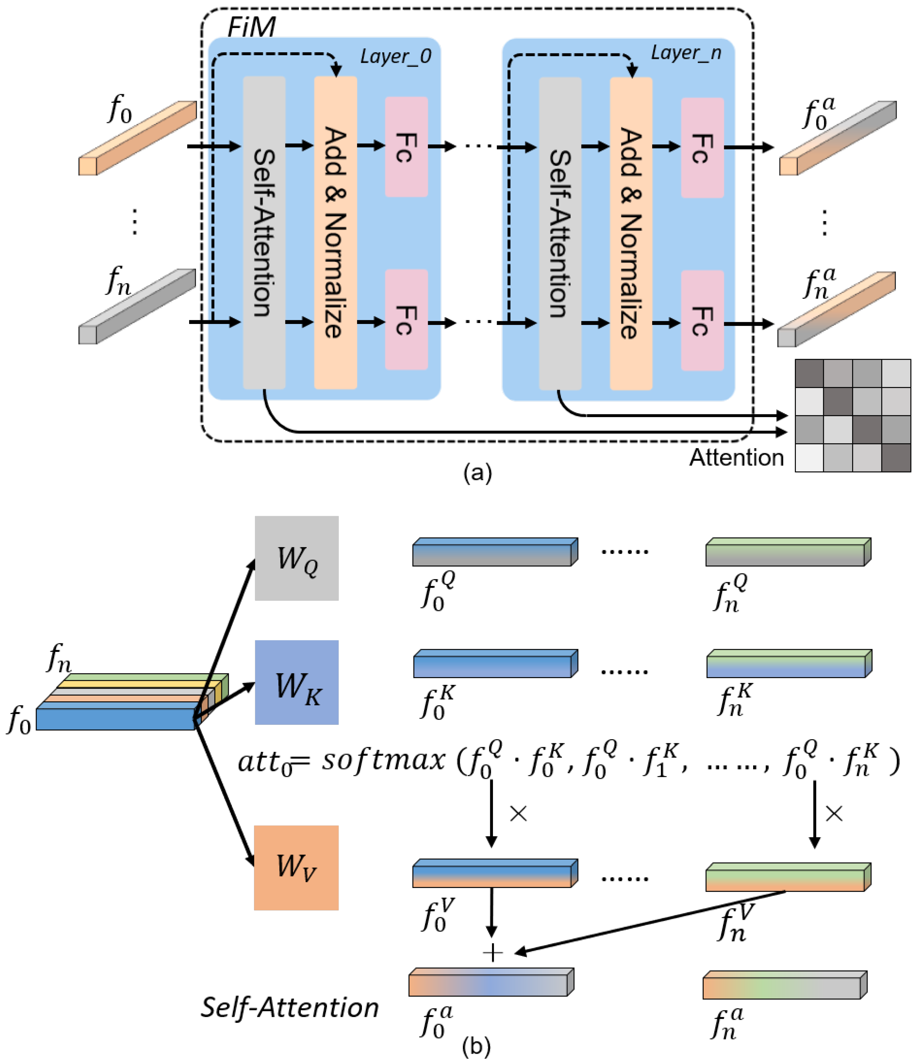
In the feature extraction process of the RSSGG_CS model, features of remote sensing images are extracted from different dimensions by different branches. The model will extract three types of features for each object in remote sensing images: (1) the object category features, (2) the visual features, and (3) the segmentation results’ morphological features. To represent the features of different modes as unified feature vectors, the above three features are processed by three feature extraction branches.

The first is the object category semantic embedding branch, corresponding to the first branch in Figure 2, which maps the category label of each instance in the image to their semantic vector, that is: $w_i=E\left(l_i\right),l_i\in \mathit{L}$, where $\mathit{L}$ is the set of words for all object category labels. We use the Skip–Gram model [39] as the wording embedding function E, and $w_i\in {\mathbb{R}}^{80}$ is the word vector corresponding to $l_i$.

The second is the visual feature extraction branch corresponding to the second branch in Figure 2, which extracts visual features of each object by convolution on remote sensing images. In the RSSGG_CS model, the object proposals are generated according to the segmentation maps of the remote sensing images. Then the proposals will be input into the network to form vectors with uniform dimensions, as follows:

$$v_i=L\left(Conv\left(r_i\right)\right),$$

(1)

where $r_i\in {\mathbb{R}}^3$ and $v_i\in {\mathbb{R}}^{300}$ are the proposal and the encoded visual feature of the object i in a remote sensing image, and $Conv$ and L represent convolutional layers [40,41] and fully connected layers, respectively. The kernel size in the convolutional layers is 3 × 3, and the activation function is ReLU. There are three convolutional layers in each $Conv$ function.

The third is the segmentation results morphological feature encoding branch, corresponding to the third branch in Figure 2, which encodes the morphology of each instance as a vector. In this paper, we directly perform convolution operations on the segmentation results of each instance in remote sensing images to extract their morphological features, as follows:

$$m_i=L\left(Conv\left(S\left(I_i\right)\right)\right),$$

(2)

where $I_i$ is the remote sensing image i, and S represents the segmentation algorithm. $Conv$ and L represent convolutional layers and fully connected layers. $m_i\in {\mathbb{R}}^{300}$ is the encoded vector for each object segmentation result. In this way, the morphological features of each instance can be extracted based on the input of segmentation results of remote sensing images by the RSSGG_CS model.

After completing the extraction and normalized representation of the three above-mentioned pattern features, it is necessary to combine them reasonably. To enhance the visual features of objects, the semantic embedding of object category label $w_i$ and visual feature $v_i$ are first connected. Then, the morphological features of object $m_i$ will be integrated together as the input of FiM module. The feature fusion process is as follows:

$$f_i=L\left(Concat(Conv\left(m_i\right),L\left(Concat(w_i,v_i)\right))\right),$$

(3)

where $f_i\in {\mathbb{R}}^{680}$ is the comprehensive feature that will be input into the FiM module. $Concat$ means concatenating two vectors together. Thus far, we have completed the extraction process of features of different dimensions, and then the attention will be calculated by the FiM.

2.3. The FiM Module

To integrate contextual information for each instance, the attention between objects needs to be calculated by the FiM module. After the FiM module, objects will be combined and sorted according to the attention between them. The complexity of subsequent predictions could be significantly reduced by filtering out combinations with smaller attention. The FiM module is designed based on an adjusted transformer architecture as shown in Figure 3. The attention between objects calculated in the FiM model will be used as part of the loss function, which is an essential reference for judging whether there is an actual semantic relationship between two objects. The attention of other instances relative to instance i will be represented as follows:

$$at{t}_i=softma{x}_{j=0}^m\left(\frac{f_i{W}_Q\times {\left(f_j{W}_K\right)}^{\mathrm{T}}}{\sqrt{d_k}}\right),$$

(4)

where $at{t}_{ij}$ represents the effect of instance j on instance i. $W_Q$ and $W_K$ are projection matrices that project the visual features into the semantic space; $d_k$ is a scaling factor. m represents that there are m instances in the current image. The semantic correlation can be calculated by the function. A larger $at{t}_{ij}$ indicates a more significant association between subject${}_i$ and object${}_j$, with an increased likelihood that there is an actual semantic relationship between them. A matrix consisting of all $att$ will be used to calculate the loss together with the binary labels y; as shown in Figure 3a, the loss function is:

$$Los{s}_1=-\frac{1}{{(m+1)}^2}\sum _{i=0}^m\sum _{j=0}^m[y_{ij}log\left(at{t}_{ij}\right)+(1-y_{ij})log(1-at{t}_{ij})],$$

(5)

Then, each comprehensive vector $f_i$ will fuse all other object features according to $at{t}_{i\ast }$, as follows:

$$f_i^a=\sum _{j=0}^{m}softmax(\frac{f_i{W}_Q\times {\left(f_j{W}_K\right)}^{\mathrm{T}}}{\sqrt{d_k}})·f_j{W}_V+f_i,$$

(6)

where $f_i^a$ is the vector of object i after fusing contextual information. $W_Q$, $W_K$, $W_V$, and $d_k$ are the same as in function (4). In this way, the contextual information is incorporated into $f_i$, and the process is clearly shown in Figure 3b. After weighted summation of all instance features, the features of $f_i$ will be fused again to avoid excessive weakening of the current object features.

2.4. Importing Statistical Knowledge as Supervision

Commonsense knowledge is an important support for human cognition and reasoning. In the task of scene graph generation, reasonably importing statistical knowledge can significantly alleviate the blindness of model predictions. Generally, there are two ways to introduce external knowledge into the model: enhancing the feature representation of objects or optimizing the model as supervision. In the RSSGG_CS model, we have used the latter. The statistical knowledge we used comes from the dataset used to train the model and the textual data from Wikipedia.

To get the distribution of relationships in the training set, we count the frequency of predicates describing the semantic relationships of each type of object combination in it. The relationship distribution can be represented as $\mathit{R}=\{r_0,...,r_{n\times (n-1)}\}$, $r_i=\{r_i^1,...,r_i^q\}$, $r_i^{*}=softmax(p_i^{*}/T)$, where $p_i^{*}$ is the number of the *th predicate that describes the relationship for object pair <subject, object>${}_i$. T is the hyperparameter used to smooth the distribution. Since the relationships of some object pairs are inherent, and their distributions are independent of the dataset, the predicate distribution of the test set and training set should be consistent. Using the KL divergence of the predicate distribution between the training set and the predicted outputs as the loss function allows the model to quickly output correct predictions.

To enrich the statistical knowledge, we integrate the external commonsense knowledge into the distribution of the training set. The commonsense knowledge is derived from the Wikipedia textual data, which contains a large number of sentences. Since the textual data contains more instance names and predicates describing relationships, we are only interested in a small part of them. We need to clean them using the category labels and predicates in the training set as reference. The similarity between words can be measured by the semantic distance between them. Therefore, in this paper, Gensim [42] is used to calculate the semantic distance between the baseline words and those in the textual data, which obtains a unified semantic representation of words by their statistical properties. Firstly, the semantic distance between those object category labels in the training set and the object names in the textual data is calculated. The sentence is filtered out if the semantic distance of all nouns in a sentence is greater than the threshold. Then, all words with semantic distance less than the threshold are replaced with their corresponding category label nouns, as follows:

$$t_{*}=\left\{\begin{array}{cc}{l}_i,\hfill & dis(l_i,t_{*})<th,\hfill \\ \mathrm{filter}\mathrm{out},\hfill & dis(l_i,t_{*})\ge th,\hfill \end{array}\right.$$

(7)

where $l_i\in \mathit{L}$ is one of the category labels, and $t_{*}\in \mathit{T}$ are the words in textual data. $dis(l_i,t_{*})$ represents the minimum semantic distance between $l_i$ and $t_{*}$, and $th$ is the threshold. The same operation is performed for the words in the textual data using the predicates in the training set as reference. In this way, the remaining sentences in the textual data have high semantic similarity with the triples <subject-predicate-object> in our training data set. The statistical knowledge used for training has been dramatically expanded. After that, using these sentences, we count the frequency of different predicates in each type of object pair <subject, object>, similar to $\mathit{R}$. To fuse the statistical knowledge of the training set and textual data for the same object pairs, we directly add up the number of different predicates obtained from the two data sources. The merged statistical knowledge is expressed as $\hat{\mathit{R}}$.

This statistical knowledge will be used with the distribution of the model output to calculate the KL-divergence $D_{kl}(\hat{\mathit{R}}|\mathit{P})$, which enables constraints on the model. The loss between the labels of object pairs relationships and the model predicted output is calculated using cross entropy $H(\mathit{Y},\mathit{P})$. Thus, the loss function of RSSGG_CS is:

$$Los{s}_2=(1-\beta -\alpha )H(\mathit{Y},\mathit{P})+\beta D_{kl}(\hat{\mathit{R}}|\mathit{P})+\alpha Los{s}_1,$$

(8)

where $\beta$ and $\alpha$ will change with epoch, which changes the weight of each part as the training progresses. The $\mathit{Y}$ and $\mathit{P}$ are the predicate label and the predicted output by the model for the relationship of an object pair, respectively. In this way, the statistical knowledge is incorporated into the RSSGG_CS model in the form of supervision.

3. Experimental Results and Discussion

The experimental approaches and the dataset for training the RSSGG_CS model are described carefully in this section. Each part of the RSSGG_CS model was experimentally validated in detail and compared with other methods, and the experimental results were analyzed deeply.

3.1. Implementation Details

We conducted our experiments on the dataset S2SG, which is the first dataset of remote sensing image scene graph generation based on segmentation results. The remote sensing images in the S2SG were taken from the WHDLD dataset [43], a widely used dataset for remote sensing image segmentation. In the S2SG dataset, the instances in remote sensing images are distinguished manually, and the relationships between them are labeled in detail. The resolution of images is $256\times 256$, and there are 128 images and 100 images in the training set and test set, respectively. Because there are rich semantic relationships between instances in remote sensing images, there are 1200 predicates in the training set. It is worth noting that the number of each predicate is consistent in training set to allow the model to more fully learn the features of different semantic relationships. Such an annotation method reduces the impact of data bias on the model. Furthermore, the relationships between objects in the test set are fully annotated to more fully validate the performance of the model. In the dataset, there are 6 categories: ‘bare soil’, ‘building’, ‘pavement’, ‘road’, ‘vegetation’ and ‘water’. There are also 12 relationship types: ‘through’, ‘stretch’, ‘surround’, ‘across’, ‘top’, ‘blend’, ‘parallel’, ‘inlaid’, ‘right’, ‘left’, ‘below’ and ‘semi-surround’. This paper uses the segmentation results to locate the objects in remote sensing images and represent their morphological features. Therefore, each object was labeled by the segmentation result in the dataset, as shown in Figure 1b, not the bounding boxes as other datasets used in scene graph generation.

When training the model, given an image, the categories of all the labeled instances in the image, the image sub-regions corresponding to the instances, and their corresponding segmentation results were input into the corresponding branches to extract features of different patterns. After fusing the features of each instance by the FiM model, the features of the instances were combined in pairs and input to the fully connected layer to predict the relationship predicate between the current two instances. The prediction results of the current object pair, their predicate label, and the statistical frequency of each predicate of the current instance pair were jointly input into the loss function to calculate the loss. During testing, the instances segmented from the remote sensing images were fed into the model in the form of three branches of the model. Eventually, the model predicted the relational predicates corresponding to each object pair. For the object pairs without semantic relationships, the prediction result was none. In our experiments, the batch size was 1, and the epoch was set to 800. The learning rate was set to ${10}^{-5}$.

To evaluate the performance of our method, the recall@K (R@K) [6] and mean recall@K (mR@K) [44] were used as the evaluation metrics. The proportion of the correct relationships among the top K confident predictions was computed to get the R@K. The average of each type of predicate R@K on the entire dataset was calculated to get the mR@K, which has the ability to more comprehensively measure whether the model can detect every kind of relationship. The computer configuration used for all experiments was: Pytorch1.10, Python3.6, an RTX 2080Ti GPU and a 2.3GHz CPU on Ubuntu16.04.

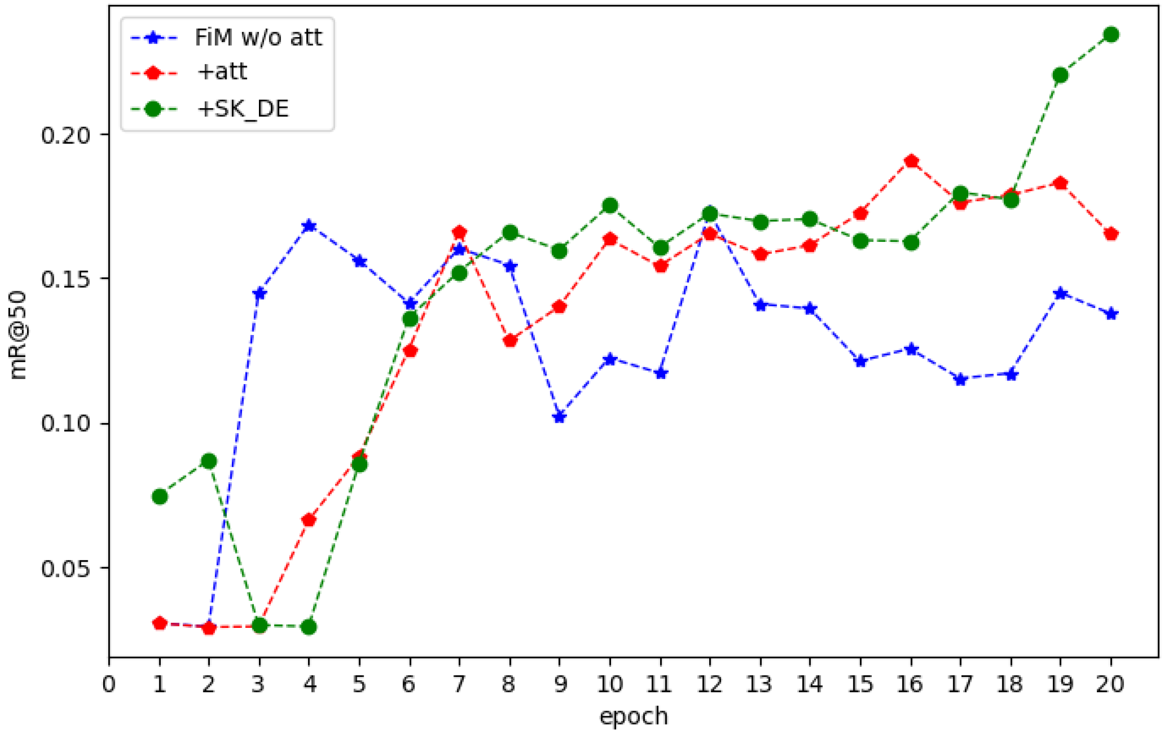
3.2. Ablation Studies

To verify the effect of each component on the model performance, we tested different combinations of submodules, as shown in

Table 1. Comparison among different combinations of submodules in RSSGG_CS.

Sub_Module	R@50	mR@50	R@20	mR@20
VF	0.2499	0.2355	0.1837	0.1332
+ WE	0.2642	0.2450	0.1900	0.1396
+ WE + MF	0.3131	0.2682	0.2257	0.1838
+ WE + MF + FiM	0.3074	0.2745	0.2281	0.1469
+ WE + MF + FiM + SK_D	0.3044	0.2795	0.2256	0.1639
+ WE + MF + FiM + SK_E	0.3248	0.2666	0.2412	0.1579
+ WE + MF + FiM + SK_DE	0.2915	0.2820	0.2204	0.1894
+ WE + MF + FiM + SK_DE_SEG	0.3040	0.2386	0.2260	0.1707

. VF represents the visual features of objects in remote sensing images, which corresponds to the second branch of Figure 2 and is the baseline of our experiments. WE are the word embeddings of object categories corresponding to the first branch of Figure 2. The morphological features of each object are represented by the MF, such as the third branch of Figure 2. FiM is the filter module to filter the object pairs without semantic relationships. SK_D, SK_E, and SK_DE represent the statistical knowledge imported into the model from the training dataset, external text, and both, respectively. The SEG represents the segmentation results used in the third branch, which are generated by the segmentation algorithm LANet [45].

Comparing the first three rows in Table 1, the metrics obviously increase with more modal features of object pairs fed into the model, especially the inputting of MF. This indicates that the morphological characteristics of instances in remote sensing images play a decisive role in the semantic relationships between them. Different modal features provide rich clues for the model to predict the semantic relationship between objects. The introduction of FiM fuses global features of the whole image for each object while suppressing pairs of instances with no semantic relationships. It causes an increase in mR@50 and R@20 but a decrease in mR@20 and R@50. These changes may be because FiM allows the model to predict more semantic relationships of object pairs correctly but suppresses the prediction scores of relational predicates, reducing the number of correctly predicted semantic relations in the top 20. It also shows that fusing contextual information makes the object contain the surrounding instance features and reduces the characteristics of the object itself. The SK_D lightly increases the mR@50 and mR@20, indicating that the model predicts the predicates of object pairs with higher prediction scores. SK_E is the statistical knowledge of the external text, which obviously increases the R@50 and R@20, indicating that a richer common knowledge allows the model to make more comprehensive predictions. SK_DE integrates the statistical knowledge of the dataset and external text into the model, achieving the best performance. Statistical knowledge as prior information greatly reduces the blindness of the model when searching the semantic space while making it easier for the model to generate high-frequency predicates. The last row shows the model performance after replacing the artificial segmentation labels of the remote sensing images in the third branch of the model with the results generated by the segmentation algorithm, which leads to a decrease in mR@K and an increase in R@K. The decrease in mR@K is because some small instances in the semantic labels of remote sensing images generated by the segmentation algorithm are challenging to be presented entirely. Their morphological characteristics have significantly changed, resulting in a significant decrease in the prediction scores of some predicates, such as ‘across’. In summary, reasonably introducing statistical knowledge to the model and fusing contextual information can significantly improve its performance in generating scene graphs of remote sensing images.

The trends of mR@50 with a different configuration of RSSGG_CS in the first 20 epochs is shown in Figure 4. The blue line indicates that the model only introduces the transformer structure for fusing contextual information but does not output the calculated attention as supervision for filtering instance pairs without semantic relations; that is, the $\alpha$ in Equation (8) is 0. The red line indicates that the $\alpha$ is set at 0.01. The green line represents the complete RSSGG_CS structure; that is, the contextual information and statistical knowledge are fused into the model. It can be seen that the introduction of the supervision of the attention can make the model more stable and obtain better performance faster. This shows that using attention as supervision can filter out many object pairs without actual semantic relationships, reducing the number of object pairs for which the model needs to predict semantic relationships. The addition of statistical knowledge makes the model performance more excellent, and its upward trend is more prominent. This trend shows that statistical knowledge indicates the direction of convergence for the model and contains a wealth of commonsense knowledge. During training, when the epoch is less than 10, $\alpha$ and $\beta$ in function (8) are set to 0.01; after that, both are set to 0. In this way, the output of the model can be quickly restricted to the expected semantic space, which significantly reduces the blindness of its search. After the model’s predictive ability is enhanced, setting $\alpha$ and $\beta$ to 0 can avoid the side effects of macro statistical knowledge on individual case prediction. The prediction of each type of relational predicate is shown in Figure 5. Even though the number of each relational predicate is consistent in the training set, their mR@50 still differed significantly. This indicates that each relational predicate is different in terms of learning difficulty and the richness of the semantic information it contains.

Scene graph generation of the natural scenes can be generally divided into three subtasks: (1) predicate classification (PreCl): predicting the predicate between two instances, given the ground truth locations and categories of the objects; (2) phase classification (PhaCl): predicting the classes and the predicates of object pairs, given the ground truth locations of objects; (3) scene graph generation (SGG): detecting the objects and relationships between them simultaneously [6,33,44]. As with the scene graph generation task for natural scenes, we also tested RSSGG_CS on the three subtasks of scene graph generation, as shown in

Table 2. The performance of RSSGG_CS on the three subtasks of scene graph generation.

PreCl		PhaCl		SGG
mR@50	mR@20	mR@50	mR@20	mR@50	mR@20
0.2820	0.1894	0.2769	0.1566	0.2419	0.1489

. In the first subtask, PreCl, the original image, the embedding of the instance category, and the instances’ location were fed into the model. In the scene graph generation of natural scenes, the bounding boxes were used to locate the objects. However, the morphological features of instances in remote sensing images were decisive for the semantic relationship between them, so the segmentation results of the objects were used to do their localization in this work. In the second subtask, PhaCl, the embeddings of instance categories were removed in the model’s input. The images were firstly fed into the segmentation algorithm in the third subtask SGG. Then, the segmentation results generated by the segmentation algorithm and the original images were simultaneously input into the model to generate the scene graphs. It can be seen that the category semantic embedding of the instance and the performance of the segmentation algorithm have a significant impact on the generated scene graph.

3.3. Comparison Experiments

Furthermore, we compared our RSSGG_CS model and other scene graph generation algorithms. The performance of RSSGG_CS and previous models for remote sensing image scene graph generation is shown in

Table 3. Comparison between previous models and RSSGG_CS for remote sensing image scene graph generation.

Model	mR@50	mR@20
VCTree	0.1261	0.0915
MOTIFS	0.0707	0.0447
IMP	0.0628	0.0480
SRSG	0.2561	0.1602
RSSGG_CS	0.2820	0.1894

. The first three are VCTree [26], MOTIFS [27], and IMP [24], which are classical algorithms for scene graph generation in natural scenes. The fourth is the model specifically designed for remote sensing image scene graph generation, which only uses the encoded morphology features to generate the scene graphs of remote sensing images. As with SRSG, we make appropriate adjustments to the inputs of the first three models to enable them to use the segmentation results of remote sensing images as inputs. The comparison shows that our model far outperforms the first three algorithms on two metrics. The first three models take only the original images and the bounding boxes of objects as input. The latter two methods also take the segmentation result as a supplement to the input and achieve superior performance. Such comparison results also show that the refined annotation of complex scenes is a prerequisite for fully understanding its content. For scene graph generation, the panorama annotation is crucial, but there is no such designed dataset at present. This will be one of the focuses of our further research. The RSSGG_CS model also has significant advantages over the SRSG model. Such results indicate that fusing contextual information allows instances to interact with surrounding objects better, and the introduction of statistical knowledge makes the model more targeted in predicting relational predicates.

To clearly present the scene graph of remote sensing images generated by our RSSGG_CS model, the visualization results are given in Figure 6. Compared with natural scenes, the semantic relationships among instances in remote sensing images are more complex because the instances have more complex morphology features. Some predicates such as ‘inlaid’ and ‘through’ are more easily to predict, but some are hard, such as ‘stretch’, for which they are difficult to define clearly. It is not easy to strictly distinguish different individuals between instances of the same category, making scene graph generation of remote sensing images more challenging. Therefore, generating the scene graphs of remote sensing images based on the segmentation results is more reasonable. Fusing the contextual information enhances the feature representation of objects, and the attention calculated by the FiM makes the model focus on the current instance. The prior information embedded in the statistical knowledge enables the model to have the expected optimization direction when faced with different instance pairs. These methods significantly reduce the difficulty for the RSSGG_CS model to mine the semantic information between objects in remote sensing images. It is worth noting that the graph structure with “nodes” and “edges” unifies the representation of different modal information. This allows us to integrate more complex external information into the generated scene graph to perform higher-level tasks like decision making.

4. Conclusions

In this paper, we propose the RSSGG_CS model for the scene graph generation task of remote sensing images. The contextual information and statistical knowledge are fused into the model to accurately predict the semantic relationships between objects in remote sensing images. Multiple modal information is fed into the RSSGG_CS model to make it easier to distinguish the characteristics of different instances. The transformer-based FiM model integrates contextual information for each object. The attention calculated by it represents the degree of association between instances, which is an essential reference for judging whether there is a semantic relationship between objects. FiM greatly enhances the feature extraction capability of the model and enhances its accuracy in predicting relational predicates between instances. The introduction of statistical knowledge from the training dataset and commonsense constrains the search space of the model and improves the quality of its generated scene graphs while accelerating the convergence of the model. Rational incorporation of statistical knowledge and fusion of global information are important means to generate remote sensing image scene graphs. In the subsequent study, we will investigate how to incorporate pre-trained visual knowledge for the model to understand remote sensing scenes better.

References

1. Redmon, J.; Divvala, S.; Girshick, R.; Farhadi, A. You only look once: Unified, real-time object detection. In Proceedings of the IEEE Conference on Computer Vision and Pattern Recognition, Las Vegas, NV, USA, 27–30 June 2016; pp. 779–788. [Google Scholar]
2. Ren, S.; He, K.; Girshick, R.; Sun, J. Faster r-cnn: Towards real-time object detection with region proposal networks. Adv. Neural Inf. Process. Syst. 2015, 28, 91–99. [Google Scholar] [CrossRef] [PubMed] [Green Version]
3. He, K.; Gkioxari, G.; Dollár, P.; Girshick, R. Mask r-cnn. In Proceedings of the IEEE International Conference on Computer Vision, Venice, Italy, 22–29 October 2017; pp. 2961–2969. [Google Scholar]
4. Liu, S.; Qi, L.; Qin, H.; Shi, J.; Jia, J. Path aggregation network for instance segmentation. In Proceedings of the IEEE Conference on Computer Vision and Pattern Recognition, Salt Lake City, UT, USA, 18–23 June 2018; pp. 8759–8768. [Google Scholar]
5. Qi, M.; Li, W.; Yang, Z.; Wang, Y.; Luo, J. Attentive relational networks for mapping images to scene graphs. In Proceedings of the IEEE/CVF Conference on Computer Vision and Pattern Recognition, Seoul, Korea, 27 October–2 November 2019; pp. 3957–3966. [Google Scholar]
6. Lu, C.; Krishna, R.; Bernstein, M.; Fei-Fei, L. Visual relationship detection with language priors. In European Conference on Computer Vision; Springer: Cham, Switzerland, 2016; pp. 852–869. [Google Scholar]
7. Li, Y.; Ouyang, W.; Zhou, B.; Wang, K.; Wang, X. Scene graph generation from objects, phrases and region captions. In Proceedings of the IEEE International Conference on Computer Vision, Glasgow, UK, 23–28 August 2017; pp. 1261–1270. [Google Scholar]
8. Mi, L.; Chen, Z. Hierarchical graph attention network for visual relationship detection. In Proceedings of the IEEE/CVF Conference on Computer Vision and Pattern Recognition, Seattle, WA, USA, 14–19 June 2020; pp. 13886–13895. [Google Scholar]
9. Wei, M.; Yuan, C.; Yue, X.; Zhong, K. Hose-net: Higher order structure embedded network for scene graph generation. In Proceedings of the 28th ACM International Conference on Multimedia, Seattle, WA, USA, 12–16 October 2020; pp. 1846–1854. [Google Scholar]
10. Gu, J.; Zhao, H.; Lin, Z.; Li, S.; Cai, J.; Ling, M. Scene graph generation with external knowledge and image reconstruction. In Proceedings of the IEEE/CVF conference on computer vision and pattern recognition, Long Beach, CA, USA, 15–20 June 2019; pp. 1969–1978. [Google Scholar]
11. Wang, W.; Wang, R.; Shan, S.; Chen, X. Sketching image gist: Human-mimetic hierarchical scene graph generation. In European Conference on Computer Vision; Springer: Cham, Switzerland, 2020; pp. 222–239. [Google Scholar]
12. Lin, X.; Ding, C.; Zeng, J.; Tao, D. Gps-net: Graph property sensing network for scene graph generation. In Proceedings of the IEEE/CVF Conference on Computer Vision and Pattern Recognition, Seattle, WA, USA, 14–19 June 2020; pp. 3746–3753. [Google Scholar]
13. Chen, S.; Jin, Q.; Wang, P.; Wu, Q. Say as you wish: Fine-grained control of image caption generation with abstract scene graphs. In Proceedings of the IEEE/CVF Conference on Computer Vision and Pattern Recognition, Seattle, WA, USA, 16–18 June 2020; pp. 9962–9971. [Google Scholar]
14. Cornia, M.; Baraldi, L.; Cucchiara, R. Show, control and tell: A framework for generating controllable and grounded captions. In Proceedings of the IEEE/CVF Conference on Computer Vision and Pattern Recognition, Long Beach, CA, USA, 15–21 June 2019; pp. 8307–8316. [Google Scholar]
15. Antol, S.; Agrawal, A.; Lu, J.; Mitchell, M.; Batra, D.; Zitnick, C.L.; Parikh, D. Vqa: Visual question answering. In Proceedings of the IEEE International Conference on Computer Vision, Washington, DC, USA, 7–13 December 2015; pp. 2425–2433. [Google Scholar]
16. Norcliffe-Brown, W.; Vafeias, S.; Parisot, S. Learning conditioned graph structures for interpretable visual question answering. Adv. Neural Inf. Process. Syst. 2018, 31, 8343–8443. [Google Scholar]
17. Krishna, R.; Zhu, Y.; Groth, O.; Johnson, J.; Hata, K.; Kravitz, J.; Chen, S.; Kalantidis, Y.; Li, L.J.; Shamma, D.A.; et al. Visual genome: Connecting language and vision using crowdsourced dense image annotations. Int. J. Comput. Vis. 2017, 123, 32–73. [Google Scholar] [CrossRef] [Green Version]
18. Xu, P.; Chang, X.; Guo, L.; Huang, P.Y.; Chen, X.; Hauptmann, A. A Survey of Scene Graph: Generation and Application. EasyChair Preprint 2020, arXiv:submit/3111057. [Google Scholar]
19. Yu, R.; Li, A.; Morariu, V.I.; Davis, L.S. Visual relationship detection with internal and external linguistic knowledge distillation. In Proceedings of the IEEE International Conference on Computer Vision, Glasgow, UK, 23–28 August 2017; pp. 1974–1982. [Google Scholar]
20. Sun, X.; Zi, Y.; Ren, T.; Tang, J.; Wu, G. Hierarchical visual relationship detection. In Proceedings of the 27th ACM International Conference on Multimedia, Nice, France, 21–25 October 2019; pp. 94–102. [Google Scholar]
21. Zhou, Y.; Sun, S.; Zhang, C.; Li, Y.; Ouyang, W. Exploring the Hierarchy in Relation Labels for Scene Graph Generation. arXiv 2020, arXiv:2009.05834. [Google Scholar]
22. Newell, A.; Deng, J. Pixels to graphs by associative embedding. Adv. Neural Inf. Process. Syst. 2017, 30, 2171–2180. [Google Scholar]
23. Ren, G.; Ren, L.; Liao, Y.; Liu, S.; Li, B.; Han, J.; Yan, S. Scene graph generation with hierarchical context. IEEE Trans. Neural Netw. Learn. Syst. 2020, 32, 909–915. [Google Scholar] [CrossRef] [PubMed]
24. Xu, D.; Zhu, Y.; Choy, C.B.; Fei-Fei, L. Scene graph generation by iterative message passing. In Proceedings of the IEEE Conference on Computer Vision and Pattern Recognition, Honolulu, HI, USA, 21–26 July 2017; pp. 5410–5419. [Google Scholar]
25. Zareian, A.; Karaman, S.; Chang, S.F. Bridging knowledge graphs to generate scene graphs. In European Conference on Computer Vision; Springer: Cham, Switzerland, 2020; pp. 606–623. [Google Scholar]
26. Tang, K.; Zhang, H.; Wu, B.; Luo, W.; Liu, W. Learning to compose dynamic tree structures for visual contexts. In Proceedings of the IEEE/CVF Conference on Computer Vision and Pattern Recognition, Long Beach, CA, USA, 16–20 June 2019; pp. 6619–6628. [Google Scholar]
27. Zellers, R.; Yatskar, M.; Thomson, S.; Choi, Y. Neural motifs: Scene graph parsing with global context. In Proceedings of the IEEE Conference on Computer Vision and Pattern Recognition, Salt Lake City, UT, USA, 18–22 June 2018; pp. 5831–5840. [Google Scholar]
28. Plesse, F.; Ginsca, A.; Delezoide, B.; Prêteux, F. Visual relationship detection based on guided proposals and semantic knowledge distillation. In Proceedings of the 2018 IEEE International Conference on Multimedia and Expo (ICME), San Diego, CA, USA, 23–27 July 2018; pp. 1–6. [Google Scholar]
29. Wang, W.; Wang, R.; Chen, X. Topic Scene Graph Generation by Attention Distillation from Caption. In Proceedings of the IEEE/CVF International Conference on Computer Vision, Montreal, QC, Canada, 11–17 October 2021; pp. 15900–15910. [Google Scholar]
30. Zhu, Z.; Luo, Y.; Wei, H.; Li, Y.; Qi, G.; Mazur, N.; Li, Y.; Li, P. Atmospheric light estimation based remote sensing image dehazing. Remote Sens. 2021, 13, 2432. [Google Scholar] [CrossRef]
31. Zhu, Z.; Luo, Y.; Qi, G.; Meng, J.; Li, Y.; Mazur, N. Remote sensing image defogging networks based on dual self-attention boost residual octave convolution. Remote Sens. 2021, 13, 3104. [Google Scholar] [CrossRef]
32. Cui, W.; Wang, F.; He, X.; Zhang, D.; Xu, X.; Yao, M.; Wang, Z.; Huang, J. Multi-scale semantic segmentation and spatial relationship recognition of remote sensing images based on an attention model. Remote Sens. 2019, 11, 1044. [Google Scholar] [CrossRef] [Green Version]
33. Li, P.; Zhang, D.; Wulamu, A.; Liu, X.; Chen, P. Semantic Relation Model and Dataset for Remote Sensing Scene Understanding. ISPRS Int. J.-Geo-Inf. 2021, 10, 488. [Google Scholar] [CrossRef]
34. Zhu, Z.; Wei, H.; Hu, G.; Li, Y.; Qi, G.; Mazur, N. A Novel Fast Single Image Dehazing Algorithm Based on Artificial Multiexposure Image Fusion. IEEE Trans. Instrum. Meas. 2021, 70, 1–23. [Google Scholar] [CrossRef]
35. Liu, Y.; Han, J.; Zhang, Q.; Shan, C. Deep Salient Object Detection With Contextual Information Guidance. IEEE Trans. Image Process. 2020, 29, 360–374. [Google Scholar] [CrossRef] [Green Version]
36. Vaswani, A.; Shazeer, N.; Parmar, N.; Uszkoreit, J.; Jones, L.; Gomez, A.N.; Kaiser, Ł.; Polosukhin, I. Attention is all you need. Adv. Neural Inf. Process. Syst. 2017, 30, 5998–6008. [Google Scholar]
37. Chen, T.; Yu, W.; Chen, R.; Lin, L. Knowledge-embedded routing network for scene graph generation. In Proceedings of the IEEE/CVF Conference on Computer Vision and Pattern Recognition, Long Beach, CA, USA, 16–20 June 2019; pp. 6163–6171. [Google Scholar]
38. Su, W.; Zhu, X.; Cao, Y.; Li, B.; Lu, L.; Wei, F.; Dai, J. Vl-bert: Pre-training of generic visual-linguistic representations. arXiv 2019, arXiv:1908.08530. [Google Scholar]
39. Mikolov, T.; Chen, K.; Corrado, G.; Dean, J. Efficient estimation of word representations in vector space. arXiv 2013, arXiv:1301.3781. [Google Scholar]
40. LeCun, Y.; Kavukcuoglu, K.; Farabet, C. Convolutional networks and applications in vision. In Proceedings of the 2010 IEEE International Symposium on Circuits and Systems, Paris, France, 30 May–2 June 2010; pp. 253–256. [Google Scholar] [CrossRef] [Green Version]
41. Lecun, Y.; Bottou, L. Gradient-based learning applied to document recognition. Proc. IEEE 1998, 86, 2278–2324. [Google Scholar] [CrossRef] [Green Version]
42. Řehůřek, R. Scalability of Semantic Analysis in Natural Language Processing. Ph.D. Thesis, Masaryk University, Brno, Czech Republic, 2011. [Google Scholar]
43. Shao, Z.; Zhou, W.; Deng, X.; Zhang, M.; Cheng, Q. Multilabel Remote Sensing Image Retrieval Based on Fully Convolutional Network. IEEE J. Sel. Top. Appl. Earth Obs. Remote Sens. 2020, 13, 318–328. [Google Scholar] [CrossRef]
44. Tang, K.; Niu, Y.; Huang, J.; Shi, J.; Zhang, H. Unbiased scene graph generation from biased training. In Proceedings of the IEEE/CVF Conference on Computer Vision and Pattern Recognition, Seattle, WA, USA, 14–19 June 2020; pp. 3716–3725. [Google Scholar]
45. Ding, L.; Tang, H.; Bruzzone, L. LANet: Local attention embedding to improve the semantic segmentation of remote sensing images. IEEE Trans. Geosci. Remote Sens. 2020, 59, 426–435. [Google Scholar] [CrossRef]
Figure 1. The illustration of a scene graph for a remote sensing image. (a) The visible light remote sensing image and the corresponding segmentation result are used as the input of the RSSGG_CS model. (b,c) are the scene graph of the image in (a). The words on the edges indicate the semantic relationships between objects, and the nodes of the scene graph are represented by the pixel-level segmentation and the category nouns of the instances, respectively.
Remotesensing 14 03118 g001
Figure 2. The framework of the RSSGG_CS model. From top to bottom, on the left side of the model are the object category semantic embeddings branch, the visual feature extraction branch, and the segmentation results morphological feature encoding branch. Then, the features of different dimensions are fed into the FiM model to calculate attention and fused to predict the relationship predicates. Attention is used to compute L o s s 1 with binary labels and guide objects for combining and sorting. The L o s s 2 will be calculated using predicted output and statistical knowledge as well as labels. When testing, the predicate predicted by the model represents the semantic relationship for the current object pair, so a series of triples, <subject-predicate-object>, are generated to make up the scene graphs of the input images.
Remotesensing 14 03118 g002
Figure 3. (a) The structure of the FiM module. The attention computed at each layer is extracted and used to screen the combinations of instances for which semantic relations actually exist. (b) The process of computing attention and fusing features for n + 1 instances in an image.
Remotesensing 14 03118 g003
Figure 4. The trends of mR@50 with different structures of RSSGG_CS in the first 20 epochs.
Remotesensing 14 03118 g004
Figure 5. Prediction results for each type of relational predicate.
Remotesensing 14 03118 g005
Figure 6. The illustration for scene graphs of remote sensing images is generated based on segmentation results. Each sub-image is followed by the visible light image of the remote sensing image, the corresponding segmentation result, and the generated scene graph. The nodes of the scene graph are represented by the segmentation results of the corresponding instances, and the semantic relationships between instances are represented by the predicates on the edges. The dashed lines indicate that the model failed to predict the relational predicate correctly.
Remotesensing 14 03118 g006