Article

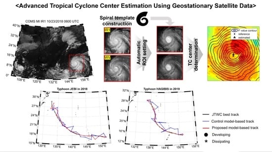
An Advanced Operational Approach for Tropical Cyclone Center Estimation Using Geostationary-Satellite-Based Water Vapor and Infrared Channels

Department of Urban & Environmental Engineering, Ulsan National Institute of Science and Technology, Ulsan 44919, Korea
*
Author to whom correspondence should be addressed.
These authors contributed equally to this work.
Remote Sens. 2022, 14(19), 4800; https://doi.org/10.3390/rs14194800
Submission received: 19 August 2022 / Accepted: 22 September 2022 / Published: 26 September 2022
(This article belongs to the Special Issue Semantic Interpretation of Remotely Sensed Images)

Abstract

:
Tropical cyclones (TCs) are destructive natural disasters. Accurate prediction and monitoring are important to mitigate the effects of natural disasters. Although remarkable efforts have been made to understand TCs, operational monitoring information still depends on the experience and knowledge of forecasters. In this study, a fully automated geostationary-satellite-based TC center estimation approach is proposed. The proposed approach consists of two improved methods: the setting of regions of interest (ROI) using a score matrix (SCM) and a TC center determination method using an enhanced logarithmic spiral band (LSB) and SCM. The former enables prescreening of the regions that may be misidentified as TC centers during the ROI setting step, and the latter contributes to the determination of an accurate TC center, considering the size and length of the TC rainband in relation to its intensity. Two schemes, schemes A and B, were examined depending on whether the forecasting data or real-time observations were used to determine the initial guess of the TC centers. For each scheme, two models were evaluated to discern whether SCM was combined with LSB for TC center determination. The results were investigated based on TC intensity and phase to determine the impact of TC structural characteristics on TC center determination. While both proposed models improved the detection performance over the existing approach, the best-performing model (i.e., LSB combined with SCM) achieved skill scores (SSs) of +17.4% and +20.8% for the two schemes. In particular, the model resulted in a significant improvement for strong TCs (categories 4 and 5), with SSs of +47.8% and +72.8% and +41.2% and +72.3% for schemes A and B, respectively. The research findings provide an improved understanding of the intensity- and phase-wise spatial characteristics of TCs, which contributes to objective TC center estimation.

Graphical Abstract

1. Introduction

A tropical cyclone (TC) is a large-scale atmospheric system caused by ocean–atmosphere interactions. When a TC forms in the open ocean, it controls the heat and mass balance between the ocean and atmosphere. Owing to its immense destructive power, a TC’s landfall often results in a significant number of fatalities and economic losses [1,2]. Due to the climatological and socioeconomic impacts of TCs, there has been a great deal of interest in understanding their behavior [3]. However, ongoing climate change and anthropogenic influences make TC behavior unpredictable, with varying TC occurrence frequencies, changes in annual TC trajectory and location with changing lifetime–maximum intensity, and an increase in the proportion of intense TCs over a lifetime [4,5,6,7]. To mitigate such uncertainty, numerical–statistical approaches, which combine several numerical models with near real-time observations, have been proposed. In particular, for 1–5-day forecasts, an ensemble with geostationary-satellite-based operational observations improved the model-based TC track forecast by 10% [8,9].
There are two steps for tracking TCs using satellite data: (1) identifying the initial guess location of a TC and (2) specifying the precise center of the TC. There are several methods for identifying the initial location of a TC in satellite images, including manual delineation, use of forecasting data, and use of the best track previously reported. Because TCs typically have distinct spatial characteristics, such as rotating comma construction [10], it is relatively easy to identify their approximate locations. Historically, manual identification of TC locations from satellite data was used [10]. However, because manual identification is operationally difficult for automated tracking of TCs, predictive fields of numerical models and extrapolated fields based on previous TC tracks have been widely used to initially estimate the location of TCs [11,12]. In the numerical-model- and extrapolated-location-based TC center estimation algorithms, a real TC center is assumed to exist close to the initial guess.
After estimating the initial position of a TC, its exact center should be determined. There are two methods for determining a TC center: wind vector analysis and cloud pattern recognition. While the former can determine the actual circulation center based on wind vectors, it requires an active sensor system and is not suitable for TC monitoring using geostationary satellite data with a high temporal resolution (e.g., hourly). The latter, on the other hand, can be used with geostationary-satellite-based observations and is widely used for operational TC center estimation systems. However, since there is no standardized automated technique for determining a TC center using cloud pattern recognition, TC center estimations are typically time-consuming and sensitive to the subjectivity of a forecaster. Owing to the discrepancies in TC data resulting from such manual processes, some researchers question the reliability of the best track determined by each regionally specialized meteorological center [13]. To overcome these limitations, several automatic TC center estimation techniques that use geostationary satellite data have been proposed.
Wimmers and Velden suggested automated rotational center hurricane eye retrieval (ARCHER), which finds a TC center considering the ring shape and brightness temperature (BT) gradient around a possible center area [14]. They utilized multifrequency microwave imagery as well as geostationary data, such as infrared and visible channel images. Jaiswal and Kishtawal [15] proposed a spiral feature extraction method that approximates the logarithmic spiral function by extracting a spiral structure from the central dense overcast region in infrared window (IRW)-channel-based TC images. Although the spiral structure of a TC is readily identifiable in strong TC events, it is ineffective in weak or dissipating TCs. Wei et al. [16] proposed a spiral-band model based on three-log spirals using IRW-based TC images. The model was validated using TCs that formed in the western North Pacific (WNP) in 2017, resulting in a mean absolute error of 0.35°. However, because the parameters for log spirals should be manually set for each TC image, this method is unsuitable for operational use. Recently, Lu et al. [12] proposed a method for determining the TC center using look-up-table-based spiral cloud belt matching (SCBeM). A TC cloud system (TCCS) was extracted from visible and IRW channel images using a simple threshold approach, and spiral template parameters were organized as a look-up table based on TC characteristics such as TC intensity, size, and tail direction.
However, previous methods have some limitations: (1) they use numerical-model-based forecasting of TC locations or extrapolated TC tracks to determine the region of interest (ROI) for a TC center, which inherently includes uncertainty; (2) the fusion of IRW and water vapor (WV) channels for objective TC center determination has received minimal attention despite the potential of WV data for the identification of convective cloud regions [17,18,19,20]; and (3) the current spiral-feature-based fitting approach identifies TC-center-like regions by averaging the BTs matching the spiral-template-fitted region and can incorrectly identify the strong convective region, such as TC outflows, as the TC center.
The purpose of this study is to investigate an advanced approach for TC center estimation using both WV and IRW channel data collected by a geostationary satellite sensor. Compared to previous research, the proposed method is novel in two aspects: (1) specifying TC candidate regions (i.e., TC ROI) using operationally available satellite observations and (2) introducing an improved spiral-pattern-fitting-based TC center estimation algorithm through an ensemble of WV and IRW channels. To reduce the uncertainty of the initial TC location estimates, circle-in-circle templates that account for the spatial characteristics of a TC according to intensity are proposed to identify the candidate region of the TC (i.e., ROI). The improved logarithmic spiral band is then used to pinpoint the precise TC center region. In this study, two schemes and two models for identifying the initial location of TCs and determining their exact locations are evaluated. The detection results are evaluated based on TC intensity and phase.

2. Data

2.1. Communication, Ocean and Meteorological Satellite Meteorological Imager

Meteorological Imager (MI) sensor data from the Communication, Ocean and Meteorological Satellite (COMS) were used to estimate TC centers. COMS, the first Korean geostationary meteorological satellite, was launched in 2010. The MI sensor has five channels that observe the Earth every 15 min: four infrared channels with a spatial resolution of 4 km, and one visible channel with a spatial resolution of 1 km (Table 1). In this study, the WV (6.7 μm) and infrared-1 (10.8 μm, IR1) channels from 2011 to 2019 were used. The spectral range of IR1 corresponds to the IRW band, which has been widely used for TC observations [21,22,23]. Since the WV channel responds to the amount of mid- to high-altitude WV and the IR1 channel responds to the cloud top’s coldness, these two channels have been widely used for quantifying convective cloud regions [16,24,25,26,27,28,29]. Because of the obscurity of the cirrus canopy, the combination of longwave infrared and WV channels contributes to the determination of TC centers [30]. Figure 1 depicts the intensity of TCs observed via the COMS WV and IR1 channels. While the regions with low BTs in the WV and IR1 channels indicate deep convection [31], the spatial distributions varied with intensity: the stronger the TC, the smaller the difference in BT between the two channels around the TC center. Compared to the IR1 observations, the normalized BT lapse rates around the TC centers were steeper for the WV observations (Figure 1c). The convection pattern was highlighted by the large difference between the deep convective region and its surroundings.

2.2. Tropical Cyclone Track Data

For operational TC monitoring, an initial TC center estimate is essential. Two types of initial guesses were employed in this study: (1) a TC center based on a numerical model forecast and (2) the previously reported TC center location, normally 6 h prior. Real-time TC warning and forecasting data from the Korea Meteorological Administration (KMA) were used to compare these two initial estimates. When a TC developed in the western North Pacific, real-time warnings were issued, based on radar and satellite observations. Numerical model-based forecasts for the next five days were issued simultaneously. Both datasets were released at 00:00, 06:00, 12:00, and 18:00 UTC, and the forecast data had a temporal resolution of 24 h. They contained the location and sea-level pressure of a TC center, maximum sustained wind speed of the TC, and radius or distance from the TC center with wind speeds greater than 15 m/s (about 29.15 knots). Real-time warning and forecasting datasets are available from the Meteorological Information Portal Service System of the KMA (http://afso.kma.go.kr/) (accessed on 7 April 2021).
There are several TC categories based on their intensity. To evaluate the proposed approach based on TC intensity, this study used the TC category by intensity, following the standards of the KMA (Table 2).

3. Methods

The proposed TC center estimation model consists of two steps: (1) setting the ROI and (2) TC center detection (Figure 2). In the first step, a square image containing a TC system was segmented from raw satellite imagery using KMA-based forecasting data and real-time track information (schemes 1 and 2). Then, clouds forming the TC with low BTs were extracted to designate the TCCS, which enabled the establishment of parameters for logarithmic spiral band (LSB) construction. Prior to matching the LSB to the TCCS, the ROI was set using a score matrix (SCM), which was proposed to eliminate regions with low probability of containing the center. In the second step, the TC center location was determined according to two models (A and B). These processes were repeated for both IRW and WV images, and the center location of the two-channel results was determined to be the final TC center. The estimation performance was evaluated using the joint typhoon warning center (JTWC) best track as the reference data.

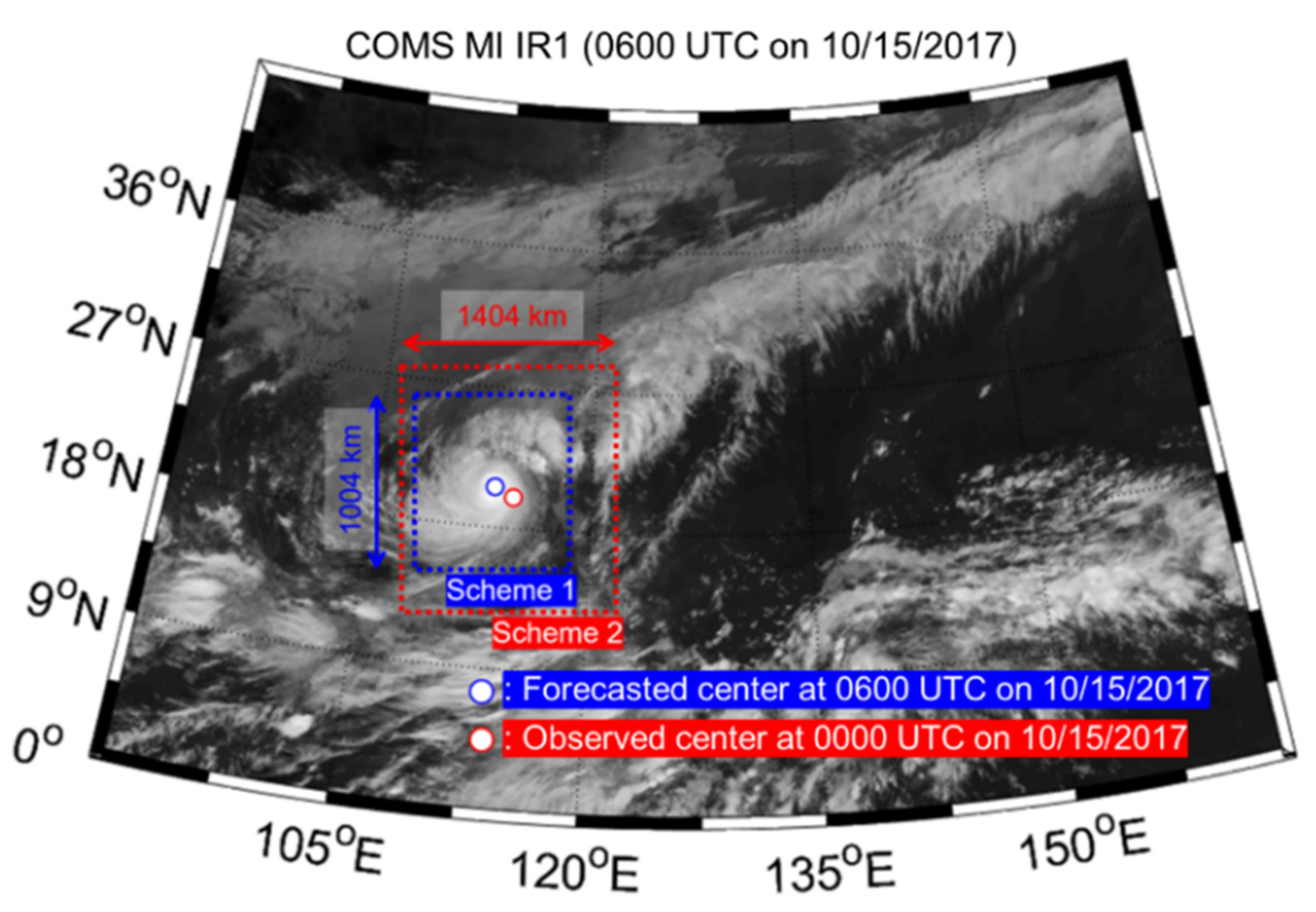
3.1. Setting Region of Interest

3.1.1. Image Segmentation Using KMA-Based Tropical Cyclone Information
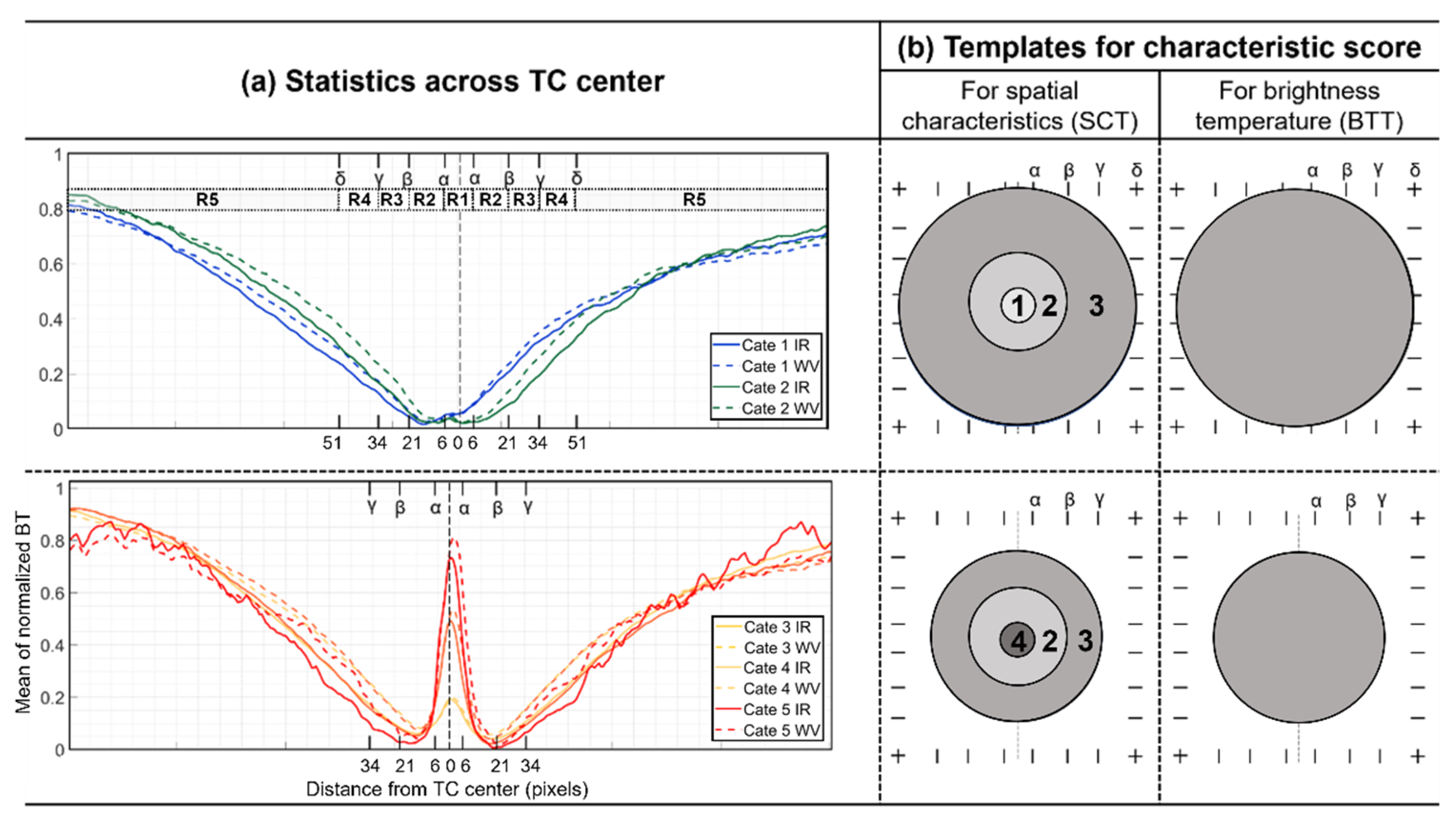
Our proposed approach consists of two schemes based on an initial guess of TC location. Scheme 1 uses the KMA-forecasting track data released 6 h prior. Scheme 2 uses the KMA-issued real-time track information for 6 h beforehand. Since the forecasting data have a 24 h temporal resolution, they were interpolated into 6 h intervals to match the real-time track. Based on the initial guess center, the candidate region of the TC center was outlined before the ROI extraction. A different ROI range was used for each scheme, owing to the difference between the two initial guesses. The ROI for scheme 1 (i.e., with forecasting data) had a side length of 251 pixels (approximately 1004 km) based on the initial guess location. Scheme 2 (i.e., with observation data) had a larger ROI with a side length of 351 pixels (estimated 1404 km) at the initial center, considering its movement over the past 6 h (Figure 3). The ROI size was based on the general coverage of TCs identified in previous studies, and the size of a TC was determined as the radius of the area with surface wind speed of 15 m/s or higher [32,33]. More than 92% of the TCs that occurred in the WNP between the years 2000 and 2005 had radii of <4.5° (about 449 km) [34].
Figure 4 depicts the TCCS extraction procedure. In the delineated region, deep convective areas with low BTs (<25% of the BT range in the region) were first identified. Subsequently, small clusters of convective areas were eliminated with the exception of the three largest clusters (Figure 4d). This process was repeated for all TC observations based on the IR1 and WV channel images.

3.1.2. Score Matrix

Prior to estimating the precise location of a TC center using LSB, it is necessary to define the ROI within the TCCS. In this study, an SCM is proposed to quantify the degree to which a region resembles the region surrounding a TC center, considering the spatial characteristics and BT of the TC. A spatially TC-like template (hereafter referred to as the spatial characteristic template (SCT)) and the region mask to the SCT (hereafter referred to as the brightness temperature template (BTT)) are proposed to obtain the SCM.
The spatial characteristics of TCs vary with their intensity. Figure 5a depicts the plot of normalized BT values across the center of the TCs by intensity category from the years 2011–2019. Based on this analysis, the BT distributions by distance from the TC center were divided into five levels: R1, R2, R3, R4, and R5. Levels R1–R5 have approximate distances of <6, 6–21, 21–34, 34–51, and 51 pixels from the TC center (1 pixel = approximately 4 km), respectively. While BT decreased toward the TC center in categories 1 and 2, it tended to be significantly elevated at R1, followed by a sharp decline at R2 and a subsequent rise from R3 in categories 3–5. The very high BT region surrounding the center (i.e., R1) indicates TC eyes [35,36]. There are distinct BT distributions within R4 and R3 with respect to weak and strong TCs, respectively. To generalize the intensity-wise spatial distribution of TCs, two types of SCT were established: a gradient-descent circle-in-circle template with radii of 6, 21, and 51 pixels in categories 1 and 2, and a gradient-descent circle-in-circle template with the highest value in the central area having radii of 6, 21, and 34 pixels. Because strong convection with a distinct spatial pattern occurs in a TC-center-like area, a BT trend employing the same-sized template to the largest radius in the SCT was used; this trend was designated the BTT. The SCT and BTT were convolved on the segmented TC observation image to generate the matrices. Figure 5b shows the two types of SCT and BTT.
Using SCT- and BTT-based matrices, an SCM was extracted to specify an ROI, a candidate region for determining the TC center. One is a correlation matrix containing two-dimensional correlation coefficient values calculated between satellite observations and SCT (referred to as CORRmat), and the other is a BT matrix containing an average of the BT values included in the BTT (referred to as BTmat). CORRmat was normalized between 0 and 1, whereas BTmat was inversely normalized between 0 and 1. SCM is defined by linearly combining the two matrices. The empirically determined coefficients of BTmat were 0.3 for a weak TC (categories 1 and 2) and 1.0 for a strong TC (categories 3–5), respectively.
Score   matrix   ( SCM ) = { C O R R m a t 1 + B T m a t 0.3 ( c a t e g o r y 2 ) C O R R m a t 1 + B T m a t 1 ( c a t e g o r y 3 )
A larger SCM value indicates a TC-center-like region. The ROI to apply LSB was defined as the region containing the top 5% of the SCM values.

3.2. Tropical Cyclone Center Determination

3.2.1. Logarithmic Spiral Band for Matching with the Tropical Cyclone Rain Band

A TCCS, as defined in Section 3.1.1, has distinct features, such as convective outflows, a rain band with a significantly strong updraft surrounding the TC center, and divergence from the center. The spiral patterns of cloud divergence around a TC center were organized qualitatively by intensity [10,37], a method that has been widely used in the operational analysis of TCs. To automate TC center detection, a logarithmic function was applied to match the divergence pattern of a TC [12,38]. In this study, an improved LSB fitting approach was proposed by fusing WV and IRW channels with KMA-based data, using the spiral band fitting approach proposed by Lu et al. [12] as a benchmark.
LSB in a TCCS can be defined using a logarithmic spiral as follows:
x = ( a ω ) e b γ cos ( θ l ) + c x y = ( a ω ) e b γ s i n ( θ l ) + c y
where x and y are the coordinates of the dots, which are the compositions of the LSB template centered at (cx, cy). The parameters a and ω determine the size and width of the logarithmic spiral, respectively. Parameter b controls the direction of the logarithmic spiral lines and θ and l control the angle and length of the LSB, respectively. The parameter γ controls the distance from (cx, cy) and is empirically defined in the range of −4–+4. Because it is challenging to set the circulation angle objectively, θ was applied in eight directions ranging 0.125–1.875 π at intervals of 0.25 π in this study. Other parameters of the spiral line (i.e., a, ω, b, and l ) were defined depending on the intensity and size of the TC. The intensity of a TC was classified into five categories according to its maximum sustained wind speed (Table 2), and its size was determined by the TCCS area. If the ratio of the TCCS area to the segmented region was less than 24%, the size was considered to be small (S). Similarly, the medium (M) and large (L) sizes were empirically defined as ratios between 24% and 26% and greater than 26%, respectively.
The LSB parameters were optimized based on the size of the TCCS and the intensity of the TC estimated by the KMA observations or forecasts (Table 3). Lu et al. (2019) proposed a spiral template with parameters suitable for their narrow ROI, defined as a square area of side length 100 km centered at the predicted center location. However, it was difficult to adhere to the previously proposed parameters because of the disparity in the segmented Image and the ROI size between the present and previous studies. In this study, the parameters were readjusted using a trial-and-error approach. The range of the parameter values used in previous studies was first examined through manual verification. Subsequently, several combinations of parameters were selected, and a random validation set was used to determine the optimum set of parameters. Parameter a was tested with a range of 20–28, and ω with a range from [0 10] to [0 15]. Parameter b was set to a tangent of 10° (about 0.17) based on the assumption from Dvorak [37] that a rain band typically has a 10° logarithmic spiral angle. Because the rain band length is closely related to TC intensity, it was set using parameter θ , ranging from [ 0   2.5 π ] to [0 3.5 π ] with increasing TC intensity [12]. The revised spiral template using the modified parameters was made smaller and optimized to fit the eyewall of a TC. This prevents the misidentification of a deep convective region, such as one that develops in the outflow of a TC, as a TC center.

3.2.2. Fitting Value for Identifying a Tropical Cyclone Center

By convolving an LSB template over the ROI, the fitting value matrix (Fmat) was calculated to identify the convective region most similar to a TC center. In this study, two Fmat extraction models were evaluated. In model A, Fmat consists of the BT averages over the region where the TCCS and LSB overlap. In model B, Fmat is the linear combination of the BT mean and SCM mean, which corresponds to the overlapped area between the TCCS and LSB. While the method of model A has been widely used in previous studies [11,12,37], model B can consider not only the BT tendency, but also the intensity-wise spatial characteristics of a TC. For model A, Fmat was calculated using the following formula:
F m a t ( i x ,   i y ) = B T   m a t c h i n g   w i t h   L S B ( i x , i y ) n
where BT matching with L S B ( i x , i y ) is the BT (K) of the pixels included in the LSB region and n is the number of matched pixels. For model B, Fmat was calculated by additionally using SCM values, excluding the dissipating TC cases for categories 1 and 2:
F m a t ( i x , i y ) = { B T   m a t c h i n g   w i t h   L S B ( i x , i y ) n ( c a t e g o r y 2 ,   w h e n   e x t i n c t i o n ) B T   m a t c h i n g   w i t h   L S B ( i x , i y ) n S C M ( i x ,   i y )
where S C M ( i x , i y ) is the SCM value for each pixel. The rain band surrounding the TC center has a colder and more uniform BT distribution than the outer region. Therefore, the region with the lowest Fmat was most likely a TC center. Since the LSB was constructed in eight directions, eight Fmats were created for each TC case. Among them, the pixel with the lowest Fmat value was identified as the TC center for both the IRW and WV images. Consequently, the final TC center was determined to be the midpoint between the two center pixels.

3.3. Accuracy Assessment

The proposed TC center estimation models were evaluated using 190 TC cases reported by the KMA from the years 2011–2019. The SCBeM was used as a control model to examine the improvement of the proposed models. The SCBeM, recently proposed by Lu et al. [12], also uses a spiral-pattern-fitting approach to determine TC centers. The comparison confirmed the efficiency of the adjusted spiral template and SCM. To evaluate the two models by the scheme, the median error (ME), mean absolute error (MAE), root mean squared error (RMSE), and percentage of MAE less than 0.5° (P05) were used. To evaluate the improvement in the performance of the proposed models compared with the control model [12], the skill score (SS) was used.
MAE = d i s t a n c e ( y , y ^ ) n
RMSE = 1 n × ( d i s t a n c e ( y , y ^ ) ) 2
P 05 = P r o p o r t i o n   o f   u n d e r   0.5 °   e r r o r
SS = ( 1 M A E m o d e l M A E c o n t r o l ) × 100
where y indicates the TC reference center reported by the JTWC-based observation and y ^ indicates the estimated center location using the proposed approach. The d i s t a n c e ( y , y ^ ) indicates the distance error between the TC reference center and estimated center. SS was considered an improvement of the proposed model compared to the control model proposed by Lu et al. [12] (2019). M A E m o d e l is the proposed-model-based MAE and M A E c o n t r o l is the control-model-based MAE. While MAE and RMSE were used for general quantitative evaluation of the models, P05 refers to the proportion of well-estimated cases where the distance error was less than 0.5°. MAE and RMSE are expressed in degrees. P05 is unitless, ranging 0–1, whereas SS is expressed as a percentage. The LSB-based TC center estimation approach relies on the structure of satellite-observed TCs, and, as a result, is highly sensitive to their intensity [10,37,39,40]. Therefore, the results were examined according to the intensity category (Table 2). In addition, the structure of a TC changes throughout its developmental phases, even when its intensity remains constant. Consequently, the proposed models were also evaluated by phase (i.e., development and extinction phases). To evaluate the performance compared to the other automatic TC center estimation methods, ARCHER [11,14], which was operationally provided by the Cooperative Institute of Meteorological Satellite Studies Group, was used. Since ARCHER utilizes the forecasting information for the initial guess center determination, the scheme-1-based models were compared to ARCHER. Because they provided their TC center estimation results for a short period of time, a total of 97 observations for 17 typhoons from the years 2018–2019 were used for comparison.

4. Results and Discussion

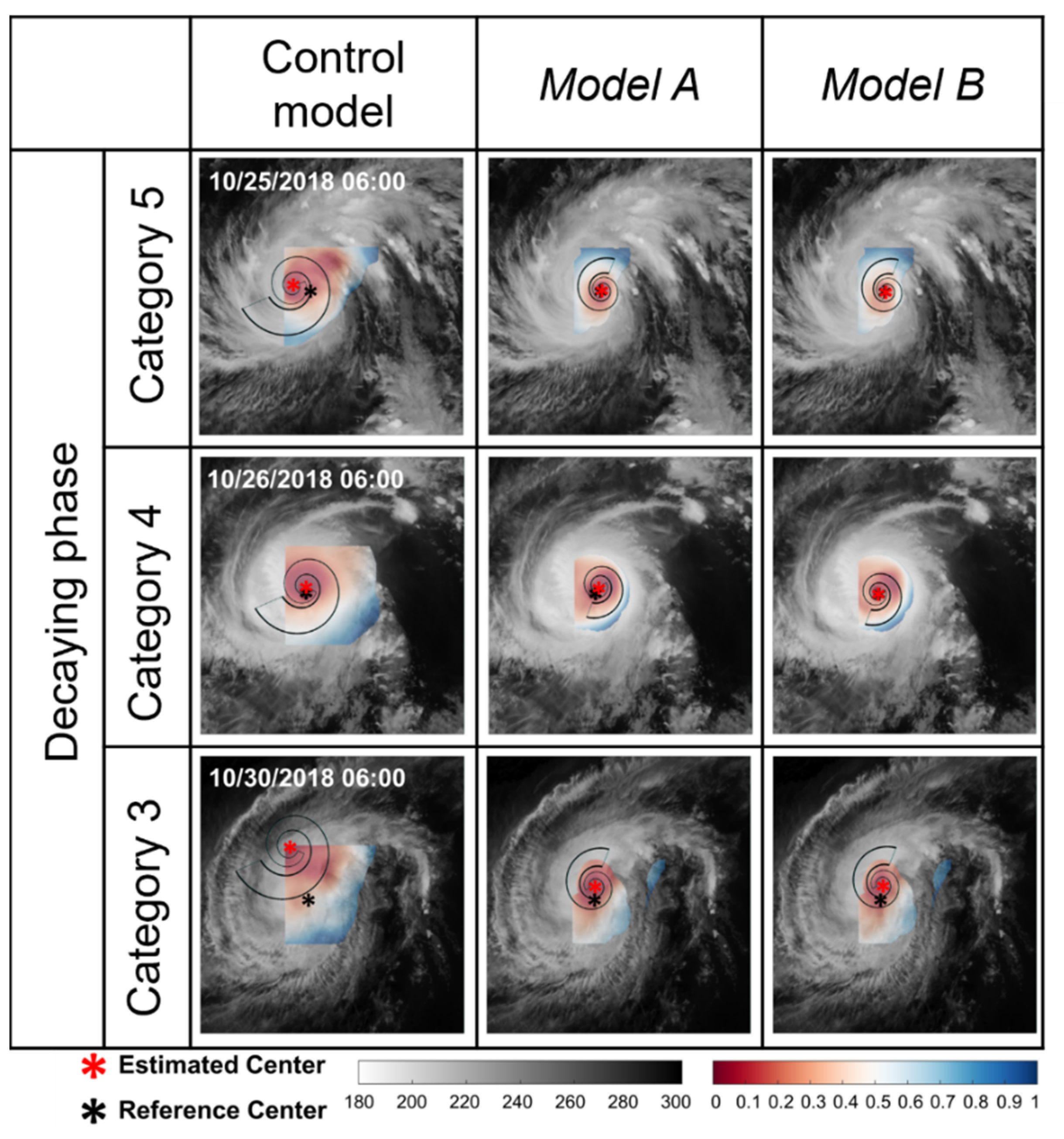
4.1. Evaluation of Tropical Cyclone Center Estimation Models by Intensity and Phase

Table 4 lists the quantitative error metrics for scheme 1 for all TC categories. In every category, model B outperformed both model A and the control model. The overall MAEs of the control model, model A, and model B were 0.53°, 0.49°, and 0.44°, respectively. Models A and B improved the performance by 6.6% and 17.4%, respectively, compared to the control model. As the TC intensified, the errors of each model decreased. In category 1, the MAEs of the control model, model A, and model B were comparable (0.59°, 0.63°, and 0.58°, respectively), whereas they were significantly different in category 5 (0.40°, 0.25°, and 0.11°, respectively). For category 5, models A and B improved the performance by 38.7% and 72.8%, respectively, compared to the control model. P05 also increased as the TC intensity increased. Model B had the highest P05, at 60%, whereas the control model had the lowest, at 44%. In particular, model B demonstrated that 84% of category 4 cases and 97% of category 5 cases were correctly identified, with MAE values <0.5°. Model B had the highest P05, 0.42, 0.49, 0.65, 0.84, and 0.97, respectively, from categories 1–5, indicating that it has a high probability of accurately pinpointing the TC center location.
The quantitative errors of the scheme-2-based TC center estimation for each category are summarized in Table 5. In scheme 2, models A and B improved the performance in terms of MAEs by 19.3% and 20.8%, respectively, compared with the control model. P05 for both models (0.27 for model A and 0.29 for model B) was more than double that of the control model (0.13). However, there were significant differences in the SS between models A and B based on intensity. In the case of weak and normal TCs with categories 1–3, the SSs in models A and B were comparable, whereas the differences were significant for the strong TC cases with categories 4 to 5: model A resulted in SSs of +3.8%, +12.5%, and +32.1% and model B resulted in SSs of +2.8%, +13.5%, and +33.8% for categories 1–3, respectively, whereas model A yielded SSs of +35.5% and +53.2% and model B resulted in SSs of +41.2% and +72.3% for categories 4 and 5, respectively. This implies that the SCM value, which was additionally used in model B, particularly contributed to the TC center determination for strong TCs. Model B detected the TC centers for 52% and 83% of the validation cases accurately, with MAE < 0.5°, whereas the control model detected only 20% and 29% of the validation cases with MAE < 0.5°. Because scheme 2 had a larger ROI than scheme 1, there was more confusion in estimating a TC center: the overall MAE of the control model based on scheme 2 was over 1°, whereas that of scheme 1 was 0.53°. However, the SSs of models A and B in scheme 2 were higher than those in scheme 1: compared to scheme 1, the overall SSs of models A and B increased by 12.7% and 3.4%, respectively, when scheme 2 was used.
Two important findings emerged from the intensity-wise evaluations of both schemes, particularly model B: (1) as the TC intensified, its MAE decreased and SS increased, and (2) the P05 values rapidly increased as the TC intensified. The combination of both SCM and LSB for extracting Fmat in model B contributed to locating an accurate TC center in both schemes.
Figure 6 compares the MAEs by intensity and phase (i.e., the developing and decaying phases of TCs). In both phases, the three models exhibited a similar pattern: the greater the TC intensity, the lower the MAE. Nonetheless, the estimation results varied considerably by phase; even within the same category, estimation errors were smaller for developing TCs than for decaying TCs. During the developing phase, model B with scheme 1 produced an MAE of 0.52° for weak TCs (categories 1–2) and 0.22° for normal and strong TCs (categories 3–5). During the decaying phase, weak TCs exhibited an MAE of 0.59°, whereas normal and strong TCs had an MAE of 0.31°. When a TC grows, the pressure gradient focused on the TC center and its structural characteristics, such as a clear storm eye in the high-pressure area and spiral inflows, are more evident than during the decaying phase [41,42].
As the TC intensifies, it becomes easier to determine its center location [12,16,43]. This is the result of the organization of the TC shape, which was affected by the pressure-gradient wind balance induced by the thermal field [44,45,46]. When the gradient increases, owing to the pressure difference between the TC center and its surroundings, the surrounding WV concentrates toward the center. In the developing phase, this causes the spatial extent of a TC to expand and convective clouds to become densely concentrated around the TC center. In contrast, the tangential wind of the inner and outer parts of a TC significantly decreases during the decaying phase because its decelerating rotation is observed using satellite data [47]. This induces phase-dependent variation in the results. In the case of scheme 1model B, the detection results in the developing phase were more accurate than those in the decaying phase, reducing the MAEs by 12.6%, 30.0%, 29.5%, 35.8%, and 27.3% for categories 1–5, respectively.
Figure 7 illustrates the TC-center-tracking results using the control model and model B according to the two schemes using typhoons JEBI (2018) and HAGIBIS (2019). Both the control model (red line) and model B (blue line) estimated the centers in the decaying phase (indicated by an asterisk) less accurately than those in the developing phase (indicated by a solid dot) (Figure 7a). While model B accurately determined the centers for both schemes, the control model generated highly variable tracks by scheme. The control model for scheme 1 followed the reference track reasonably well, whereas the model for scheme 2 yielded erratic track estimations. This implies that proposed model B is less sensitive to the initial guess center and can be used for operational purposes.
In addition, the operationally reported TC center determination results based on ARCHER [11,14] were compared with the results from the proposed models. Table 6 shows the center estimation performance of ARCHER, the scheme-1-based control model, and the proposed models (i.e., models A and B). For all TC observations (i.e., 97 observations for 17 typhoons), ARCHER, the control model, and models A and B produced MAEs of 0.45°, 0.50°, 0.46°, and 0.38 °, respectively. Similar to the previous evaluation results (Table 4 and Table 5, and Figure 6), model B resulted in the best performance, followed by model A and control model. ARCHER showed a performance comparable to that of model A.

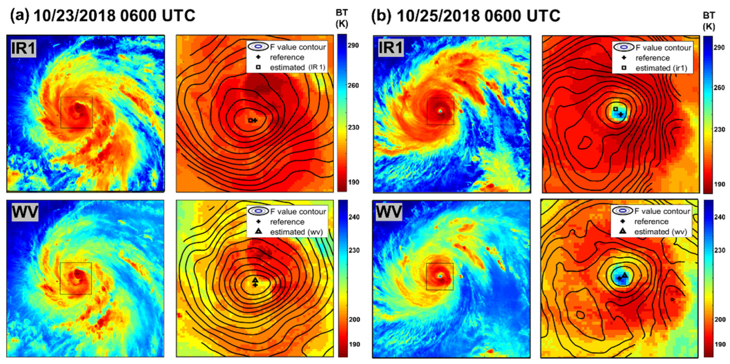
4.2. Tropical Cyclone Center Estimations Using Typhoon YUTU in 2018

Using Typhoon YUTU in 2018, the intensity- and phase-wise TC center estimation results from the three models were validated. The ROI sizes and TC center detection errors are listed in Table 7. Models A and B calculated Fmat in the ROI extracted using an SCM, whereas the control model calculated Fmat in a 125-pixel-square ROI based on the initial guess for a TC center. For Typhoon YUTU (2018), the ROI size of models A and B decreased by 31–61%, respectively, compared to the control model; therefore, the ROIs in models A and B were narrower than those of the control model. As shown in Table 7, the detection performances of models A and B are superior to those of the control model. This suggests that SCM-based ROI extraction and improved LSB contribute to the accurate detection of TC centers. Comparing the detection performance between the two proposed models, model B demonstrated more accurate detection results in the eight cases of Typhoon YUTU (2018) than the other models. It is suggested that the revised Fmat with an SCM in model B improved TC center detection. Figure 8 depicts the TC center detection results of the three models for the TCs listed in Table 7. The weaker the TC, the more likely it was for the control model to misidentify the TC outflow as a TC center, whereas models A and B detected the TC center relatively well. This is because the ROIs of the proposed models were able to exclude regions that could be incorrectly identified, such as a region with deep convection, but not a TC center region. This is evident in the case of the TCs at 0600 UTC on 30 October 2018 (category 3 TC in the decaying phase). While the outflow region was incorrectly identified as a TC center by the control model, models A and B had already excluded this region from the ROIs. In other words, the SCM helped to reduce confusion in TC center detection.
Figure 9 shows the scheme-2—model-B-based channel-wise TC observations and center estimation results for typhoon YUTU (2018). Compared to IR1 channel observations, WV-based observations showed more concentrated patterns of low BTs, which corresponded to the deep convective area. It caused the WV-channel-based F-value to appear to have a sharper gradient toward the TC-center-like region than the IR1 channel. However, due to the insignificance of the cirrus altitude in the TC system [11,40], the F-values of each channel do not always indicate the same point. Moreover, in some cases, such as Figure 9a,b, the pre-determined TC centers from each channel were positioned on different directions relative to the real TC center. This is derived from the difference between the IR1 and WV channels for deep convective regions. From the years 2011–2019, about 32% of the TC cases demonstrated that the pre-determined TC centers between IR1 and WV were located in directions that differed from the reference centers by greater than 90°. Consequently, the combination of IR1 and WV is believed to synergistically contribute to the objective TC center determination by reducing the obscurity of the cirrus canopy.

4.3. Novelty and Limitations

In this study, an improved LSB-based TC center estimation approach that exploits the spatial characteristics of a TCCS is proposed. The SCM used to quantify the spatial characteristics and BT trend of the TCCS contributed to both steps of the proposed TC center estimation approach (i.e., ROI setting and TC center determination). This enabled the identification of regions that may have been misidentified as TC centers during the ROI-setting step. Thus, specifying ROIs using an SCM can be expected to not only contribute to an increased focus on TC-like centers, but also reduce the algorithm’s running time. It was also used to extract Fmat in model B, which improves the accuracy of TC center detection. The improved LSB proposed in this study enables a better fit to the spiral-shaped rainband surrounding the TC center than the control model. This contributes positively, particularly when TC intensity is weak or moderate. It was confirmed that, while the spiral band from the control model incorrectly identified the region with low BT in outflows as a TC center, the LSB from the proposed model detected the rainband surrounding the TC center relatively well (e.g., at 22 October 2018 1200 UTC, 23 October 2018 0600 UTC, 25 October 2018 0000 UTC, and 30 October 2018 0600 UTC; Figure 8). The TC center estimation approach proposed in this study has several novelties: (1) it is fully automated and can be used for operational purposes; (2) the advanced ROI-setting process can prescreen potentially confusing regions such as outflows of the TC; and (3) the improved LSB considers the size and length of the TC rainband in relation to its intensity.
However, the proposed algorithm had several limitations. (1) It was difficult to fit the proposed LSB to rainbands in weak and decaying TCs because of the various TC shapes. In this situation, numerical weather prediction models or microwave satellite data can provide reliable center locations for weak TCs, although they cannot be obtained in real time. Ground-based weather radar is also a great way to locate a TC center within radar coverage. (2) Detection error can be caused by a large ROI, according to scheme 2 (with KMA-based observation data reported 6 h prior). This increases the likelihood that distant convective clouds will be identified as TC centers. While SCM can mitigate such erroneous TC center estimations, it has little effect on weak and decaying TCs, which have irregularly shaped clouds. Since the extent of the ROI was based on the distance that a TC could potentially travel during the data interval, reducing the report interval could reduce misidentification of TC candidate regions.

5. Conclusions

The primary objective of this study was to propose a fully automated operational TC center estimation method using geostationary satellite data. Two steps are involved in estimating TCs: (1) ROI setting and (2) TC center determination. While the majority of previous studies have focused on the second step, ROI specification is crucial for accurate and efficient TC center estimation. In this study, an SCM and improved LSB were proposed for more accurate TC center determination and ROI setting. To investigate the optimal method for TC center determination, two models were tested (models A and B) using two schemes (schemes 1 and 2). The results were compared with those of the control model [12] based on the intensity and phase of TCs using best-track reference data. Compared with the control model, the proposed models improved the performance with errors of less than 0.5°, with improvements of 10% and 16% in schemes 1 and 2, respectively. In particular, for strong TCs (category ≥ 4), the models significantly improved by 35% and 43%, respectively. Among the proposed models, model B achieved the best performance, with MAEs of 0.44° and 0.98° in schemes 1 and 2, respectively. Compared to the control model, the overall performance of model B improved by 17.4% and 20.8% for schemes 1 and 2, respectively. In particular, for Category 5, the performance of model B improved by 72.8% and 72.3% in both schemes. Compared with model A, model B improved the performance by approximately 56.0% and 39.5% for schemes 1 and 2, respectively. These results indicate that specifying the ROI using an SCM could effectively reduce false detections, and the combination of an SCM and improved LSB, proposed as model B in this study, improves the accuracy of TC center detection using geostationary satellite data.
While the proposed approach produced promising results, there is room for improving the TC center detection. Recently, deep learning has been used for TC identification using geostationary satellite data; however, it has not been explored for TC center determination from geostationary satellite images. Future work will include convolutional-neural-network-based TC center determination because TCs and their centers have distinct spatial characteristics based on their intensity and phase.

Author Contributions

Y.S. and J.L. wrote the manuscript and contributed to data analysis and research design. J.I. supervised this study; contributed to the research design, manuscript writing, and discussion of the results; and served as the corresponding author. S.S. contributed to the data analysis and model design. All authors have read and agreed to the published version of the manuscript.

Funding

This work was funded by a grant (no. 20009742) from the Ministry-Cooperation R&D program of Disaster-Safety, funded by the Ministry of Interior and Safety (MOIS), South Korea, and by “Development of Advanced Science and Technology for Marine Environmental Impact Assessment” of the Korea Institute of Marine Science and Technology Promotion (KIMST), funded by the Ministry of Oceans and Fisheries (KIMST-20210427) and by the Ministry of Science and ICT, Korea, under the Information Technology Research Center support program (IITP-2022-2018-0-01424). J.L. was partially supported by the Basic Science Research Program through the National Research Foundation of Korea (NRF), funded by the Ministry of Education of South Korea (no. 2020R1A6A3A13077532).

Data Availability Statement

COMS satellite data are available at the following website: https://datasvc.nmsc.kma.go.kr/datasvc/ (accessed on 21 April 2021). The data used in this research are available upon the request to the corresponding author.

Conflicts of Interest

The authors declare no conflict of interest.

Abbreviations

ARCHERAutomated Rotational Center Hurricane Eye Retrieval
BTBrightness temperature
BTTBrightness temperature template
COMS MICommunication, Ocean and Meteorological Satellite Meteorological Imager
IR1Infrared-1
JWTCJoint warning typhoon center
KMAKorea Meteorological Administration
LSBLogarithm spiral band
MAEMean absolute error
P05Percentage of MAE less than 0.5°
RMSERoot mean squared error
ROIRegion of interest
SCBeMSpiral cloud belt matching
SCMScore matrix
SCTSpatial characteristic template
SSSkill score
TCTropical cyclone
TCCSTropical cyclone cloud system
WNPWestern North Pacific
WVWater vapor

References

  1. Jacob, S.D.; Shay, L.K. The Role of Oceanic Mesoscale Features on the Tropical Cyclone–Induced Mixed Layer Response: A Case Study. J. Phys. Oceanogr. 2003, 33, 649–676. [Google Scholar] [CrossRef]
  2. Weinkle, J.; Maue, R.; Pielke, R. Historical Global Tropical Cyclone Landfalls. J. Clim. 2012, 25, 4729–4735. [Google Scholar] [CrossRef]
  3. Moore, T.W.; Dixon, R.W. Tropical cyclone-tornado casualties. Nat. Hazards 2012, 61, 621–634. [Google Scholar] [CrossRef]
  4. Holland, G.; Bruyère, C.L. Recent intense hurricane response to global climate change. Clim. Dyn. 2014, 42, 617–627. [Google Scholar] [CrossRef]
  5. Liang, A.; Oey, L.; Huang, S.; Chou, S. Long-term trends of typhoon-induced rainfall over Taiwan: In situ evidence of poleward shift of typhoons in western North Pacific in recent decades. J. Geophys. Res. 2017, 122, 2750–2765. [Google Scholar] [CrossRef]
  6. Altman, J.; Ukhvatkina, O.N.; Omelko, A.M.; Macek, M.; Plener, T.; Pejcha, V.; Cerny, T.; Petrik, P.; Srutek, M.; Song, J.; et al. Poleward migration of the destructive effects of tropical cyclones during the 20th century. Proc. Natl. Acad. Sci. USA 2018, 115, 11543–11548. [Google Scholar] [CrossRef]
  7. Lee, J.; Im, J.; Cha, D.-H.; Park, H.; Sim, S. Tropical Cyclone Intensity Estimation Using Multi-Dimensional Convolutional Neural Networks from Geostationary Satellite Data. Remote Sens. 2020, 12, 108. [Google Scholar] [CrossRef]
  8. Aberson, S.D. Targeted Observations to Improve Operational Tropical Cyclone Track Forecast Guidance. Mon. Weather Rev. 2003, 131, 1613–1628. [Google Scholar] [CrossRef]
  9. Dong, L.; Zhang, F. OBEST: An Observation-Based Ensemble Subsetting Technique for Tropical Cyclone Track Prediction. Weather Forecast. 2016, 31, 57–70. [Google Scholar] [CrossRef]
  10. Dvorak, V.F. Tropical Cyclone Intensity Analysis and Forecasting from Satellite Imagery. Mon. Weather Rev. 1975, 103, 420–430. [Google Scholar] [CrossRef]
  11. Wimmers, A.J.; Velden, C.S. Advancements in Objective Multisatellite Tropical Cyclone Center Fixing. J. Appl. Meteorol. Climatol. 2016, 55, 197–212. [Google Scholar] [CrossRef]
  12. Lu, X.; Yu, H.; Yang, X.; Li, X.; Tang, J. A new technique for automatically locating the center of tropical cyclones with multi-band cloud imagery. Front. Earth Sci. 2019, 13, 836–847. [Google Scholar] [CrossRef]
  13. Song, J.-J.; Wang, Y.; Wu, L. Trend discrepancies among three best track data sets of western North Pacific tropical cyclones. J. Geophys. Res. 2010, 115, D12. [Google Scholar] [CrossRef]
  14. Wimmers, A.J.; Velden, C.S. Objectively Determining the Rotational Center of Tropical Cyclones in Passive Microwave Satellite Imagery. J. Appl. Meteorol. Climatol. 2010, 49, 2013–2034. [Google Scholar] [CrossRef]
  15. Jaiswal, N.; Kishtawal, C.M. Automatic Determination of Center of Tropical Cyclone in Satellite-Generated IR Images. IEEE Geosci. Remote Sens. Lett. 2011, 8, 460–463. [Google Scholar] [CrossRef]
  16. Wei, K.; Jing, Z.-L.; Li, Y.-X.; Liu, S.-L. Spiral band model for locating Tropical Cyclone centers. Pattern Recognit. Lett. 2011, 32, 761–770. [Google Scholar] [CrossRef]
  17. Schmetz, J.; Tjemkes, S.A.; Gube, M.; van de Berg, L. Monitoring deep convection and convective overshooting with METEOSAT. Adv. Space Res. 1997, 19, 433–441. [Google Scholar] [CrossRef]
  18. Olander, T.L.; Velden, C.S. Tropical Cyclone Convection and Intensity Analysis Using Differenced Infrared and Water Vapor Imagery. Weather Forecast. 2009, 24, 1558–1572. [Google Scholar] [CrossRef]
  19. Han, H.; Lee, S.; Im, J.; Kim, M.; Lee, M.-I.; Ahn, M.H.; Chung, S.-R. Detection of Convective Initiation Using Meteorological Imager Onboard Communication, Ocean, and Meteorological Satellite Based on Machine Learning Approaches. Remote Sens. 2015, 7, 9184–9204. [Google Scholar] [CrossRef]
  20. Lee, J.; Kim, M.; Im, J.; Han, H.; Han, D. Pre-trained feature aggregated deep learning-based monitoring of overshooting tops using multi-spectral channels of GeoKompsat-2A advanced meteorological imagery. GIsci Remote Sens. 2021, 58, 1052–1071. [Google Scholar] [CrossRef]
  21. Kumar, S.; del Castillo-Velarde, C.; Rojas, J.L.F.; Moya-Álvarez, A.; Castro, D.M.; Srivastava, S.; Silva, Y. Precipitation structure during various phases the life cycle of precipitating cloud systems using geostationary satellite and space-based precipitation radar over Peru. GIsci Remote Sens. 2020, 57, 1057–1082. [Google Scholar] [CrossRef]
  22. Yin, G.; Baik, J.; Park, J. Comprehensive analysis of GEO-KOMPSAT-2A and FengYun satellite-based precipitation estimates across Northeast Asia. GIsci Remote Sens. 2022, 59, 782–800. [Google Scholar] [CrossRef]
  23. Zhou, Y.; Matyas, C.J. Regionalization of precipitation associated with tropical cyclones using spatial metrics and satellite precipitation. GIsci Remote Sens. 2021, 58, 542–561. [Google Scholar] [CrossRef]
  24. Chang, F.-L.; Li, Z. Retrieving vertical profiles of water-cloud droplet effective radius: Algorithm modification and preliminary application. J. Geophys. Res. 2003, 108, D24. [Google Scholar] [CrossRef]
  25. Fiolleau, T.; Roca, R. An Algorithm for the Detection and Tracking of Tropical Mesoscale Convective Systems Using Infrared Images From Geostationary Satellite. IEEE Trans. Geosci. Remote Sens. 2013, 51, 4302–4315. [Google Scholar] [CrossRef]
  26. Takahashi, H.; Luo, Z.J. Characterizing tropical overshooting deep convection from joint analysis of CloudSat and geostationary satellite observations. J. Geophys. Res. 2014, 119, 112–121. [Google Scholar] [CrossRef]
  27. Han, D.; Lee, J.; Im, J.; Sim, S.; Lee, S.; Han, H. A Novel Framework of Detecting Convective Initiation Combining Automated Sampling, Machine Learning, and Repeated Model Tuning from Geostationary Satellite Data. Remote Sens. 2019, 11, 1454. [Google Scholar] [CrossRef]
  28. Lee, H.-B.; Heo, J.-H.; Sohn, E.-H. Korean fog probability retrieval using remote sensing combined with machine-learning. GIsci Remote Sens. 2021, 58, 1434–1457. [Google Scholar] [CrossRef]
  29. Lee, S.; Choi, J. A snow cover mapping algorithm based on a multitemporal dataset for GK-2A imagery. GIsci Remote Sens. 2022, 59, 1078–1102. [Google Scholar] [CrossRef]
  30. Liu, C.-C.; Shyu, T.-Y.; Lin, T.-H.; Liu, C.-Y. Satellite-derived normalized difference convection index for typhoon observations. J. Appl. Remote Sens. 2015, 9, 096074. [Google Scholar] [CrossRef] [Green Version]
  31. Rosenfeld, D.; Woodley, W.L.; Lerner, A.; Kelman, G.; Lindsey, D.T. Satellite detection of severe convective storms by their retrieved vertical profiles of cloud particle effective radius and thermodynamic phase. J. Geophys. Res. 2008, 113, D4. [Google Scholar] [CrossRef]
  32. Frank, W.M.; Gray, W.M. Radius and Frequency of 15 m s−1 (30 kt) Winds around Tropical Cyclones. J. Appl. Meteorol. Climatol. 1980, 19, 219–223. [Google Scholar] [CrossRef]
  33. Cocks, S.B.; Gray, W.M. Variability of the Outer Wind Profiles of Western North Pacific Typhoons: Classifications and Techniques for Analysis and Forecasting. Mon. Weather Rev. 2002, 130, 1989–2005. [Google Scholar] [CrossRef]
  34. Lee, C.-S.; Cheung, K.K.W.; Fang, W.-T.; Elsberry, R.L. Initial Maintenance of Tropical Cyclone Size in the Western North Pacific. Mon. Weather Rev. 2010, 138, 3207–3223. [Google Scholar] [CrossRef]
  35. Wang, Y.; Wu, C.C. Current understanding of tropical cyclone structure and intensity changes—A review. Meteorol. Atmos. Phys. 2004, 87, 257–278. [Google Scholar] [CrossRef]
  36. Yang, J.; Chen, M. Variations of rapidly intensifying tropical cyclones and their landfalls in the Western North Pacific. Coast. Eng. 2021, 63, 142–159. [Google Scholar] [CrossRef]
  37. Dvorak, V.F. Tropical Cyclone Intensity Analysis Using Satellite Data; US Department of Commerce, National Oceanic and Atmospheric Administration, National Environmental Satellite, Data, and Information Service: Washington, DC, USA, 1984; Volume 11.
  38. Wong, K.Y.; Yip, C.L.; Li, P.W. Automatic tropical cyclone eye fix using genetic algorithm. Expert Syst. Appl. 2008, 34, 643–656. [Google Scholar] [CrossRef]
  39. Ming, J.; Zhang, J.A. Effects of surface flux parameterization on the numerically simulated intensity and structure of Typhoon Morakot (2009). Adv. Atmos. Sci. 2016, 33, 58–72. [Google Scholar] [CrossRef]
  40. Liu, C.; Shyu, T.; Chao, C.; Lin, Y. Analysis on typhoon Long Wang intensity changes over the ocean via satellite data. J. Mar. Sci. Technol. 2009, 17, 23–28. [Google Scholar] [CrossRef]
  41. Fujita, T.; Izawa, T.; Watanabe, K.; Imai, I. A Model of Typhoons Accompanied by Inner and Outer Rainbands. J. Appl. Meteorol. Climatol. 1967, 6, 3–19. [Google Scholar] [CrossRef]
  42. Holland, G.J. Angular momentum transports in tropical cyclones. Q. J. R. Meteorol. Soc. 1983, 109, 187–209. [Google Scholar] [CrossRef]
  43. Bai, Q.; Wei, K.; Jing, Z.; Li, Y.; Tuo, H.; Liu, C. Tropical cyclone spiral band extraction and center locating by binary ant colony optimization. Sci. China Earth Sci. 2012, 55, 332–346. [Google Scholar] [CrossRef]
  44. Willoughby, H.E. Forced secondary circulations in hurricanes. J. Geophys. Res. Oceans. 1979, 84, 3173–3183. [Google Scholar] [CrossRef]
  45. Smith, R.K. Tropical Cyclone Eye Dynamics. J. Atmos. Sci. 1980, 37, 1227–1232. [Google Scholar] [CrossRef]
  46. Willoughby, H.E. Temporal Changes of the Primary Circulation in Tropical Cyclones. J. Atmos. Sci. 1990, 47, 242–264. [Google Scholar] [CrossRef]
  47. Tsujino, S.; Horinouchi, T.; Tsukada, T.; Kuo, H.-C.; Yamada, H.; Tsuboki, K. Inner-Core Wind Field in a Concentric Eyewall Replacement of Typhoon Trami (2018): A Quantitative Analysis Based on the Himawari-8 Satellite. J. Geophys. Res. 2021, 126, e2020JD034434. [Google Scholar] [CrossRef]
Figure 1. Intensity-wise tropical cyclones observed from Communication, Ocean and Meteorological Satellite Meteorological Imager in 2017: typhoon NANMADOL with 50 kts wind speed (first row), typhoon LAN with 90 kts wind speed (second row), and typhoon NORU with 115 kts wind speed (third row). (a,b) show infrared-1- and water-vapor-channel-based images, respectively, and (c) represents the normalized brightness temperature distribution of the horizontal line with 101 pixels (approximately 404 km; dotted lines in (a,b)) across the tropical cyclone center.
Remotesensing 14 04800 g001
Figure 2. Flow chart of the proposed TC center estimation approach.
Remotesensing 14 04800 g002
Figure 3. Examples of interest regions according to the two schemes using Communication, Ocean and Meteorological Satellite Meteorological Imager observations at 0600 UTC on 15 October 2017. The blue circle is the tropical cyclone center predicted from Korea Metrological Association forecasting reports at 0600 UTC on 15 October 2017 issued 6 h prior, and the red circle is the tropical cyclone center observed at 0000 UTC on 15 October 2017. The blue and red dashed boxes are the interest regions used for schemes 1 and 2, respectively.
Remotesensing 14 04800 g003
Figure 4. Pre-processing to extract a tropical cyclone cluster system (TCCS) using Communication, Ocean and Meteorological Satellite Meteorological Imager sensor observation at 0600 UTC on 15 October 2017 as an example. (a) Brightness temperature (BT)-based infrared image observed from Communication, Ocean and Meteorological Satellite Meteorological Imager. (b) Deep convective region with a BT below the 25% quantile in the interest region. (c) Excluding the three largest clusters, the orange-colored clusters represent small fragmented clusters. (d) The extracted TCCS.
Remotesensing 14 04800 g004
Figure 5. Two spatial templates to calculate a score matrix, where (a) represents the morphological characteristics around a tropical cyclone center by intensity category. To compare the spatial distribution of the events, they were normalized into 0–1. The solid line in (a) shows a brightness temperature (BT) trend in the infrared channel and the dashed line shows a BT trend in the water vapor channel. (b) represents the templates for spatial characteristics and BT of a tropical cyclone by intensity category. The size and value of each template are decided based on statistics across the tropical cyclone center. R1–R5 (distance ranges from the tropical cyclone center) were determined using α, β, γ, and δ, representing a distance of 6, 21, 34, and 51 pixels, respectively. Each pixel size corresponds to approximately 4 km. The values of the spatial characteristic templates consist of (1,2,3) and (4,2,3) toward the outside for intensity categories 1 and 2 and 3–5, respectively.
Remotesensing 14 04800 g005
Figure 6. Mean absolute error (MAE) of the control model and models A and B for both scheme 1 (above) and 2 (below). The MAE of all models decreased as the tropical cyclone intensity increased. In both schemes, category 5 showed the best performance while category 1 yielded the largest estimation error.
Remotesensing 14 04800 g006
Figure 7. Tracking results of the control model and model B based on two schemes for typhoon JEBI in 2018 and typhoon HAGIBIS in 2019. (a,b) show the tracking results according to schemes 1 and 2, respectively. The black, blue, and red lines indicate the JTWC best track, the estimated track by the control model, and the estimated center by model B, respectively. A filled circle represents a tropical cyclone in the developing phase, while an asterisk indicates a tropical cyclone in the decaying phase.
Remotesensing 14 04800 g007
Figure 8. Tropical cyclone center location estimated by the scheme-2-based control model and models A and B by category and phase. Communication, Ocean and Meteorological Satellite Meteorological Imager infrared-1-channel-based observations are used as background images, and regions of interest are shown in color. The color of regions of interest represents normalized Fmat values (0–1) at the IRW observation, and reddish color indicates lower Fmat. The black asterisks indicate the tropical cyclones center determined by the JTWC best track and the red asterisks represent the tropical cyclone center estimated by the control model and models A and B.
Remotesensing 14 04800 g008aRemotesensing 14 04800 g008b
Figure 9. Channel-wise tropical cyclone (TC) observations and TC center estimation results for typhoon YUTU (2018). (a,b) are the TCs observed at 23 October 2018 0600 UTC and 25 October 2018 0600 UTC, respectively. The left column of (a,b) shows the IR1- and WV-channel-based observation, while the right column depicts the contour lines of the F-value for the area around the center (the black rectangle on the left column).
Remotesensing 14 04800 g009
Table 1. Specifications of the Communication, Ocean and Meteorological Satellite Meteorological Imager sensor. Water vapor and infrared 1 channels were used for tropical cyclone center estimation in this study.
ChannelWavelength Range (µm)Central Wavelength (µm)Spatial Resolution (km)Temporal Resolution (min)
Visible0.55–0.80.67115
Shortwave Infrared3.5–4.03.74
Water Vapor6.5–7.06.7
Infrared 110.3–11.310.8
Infrared 211.5–12.512.0
Table 2. Intensity categorization of tropical cyclones according to the standard from the Korea Meteorological Administration.
CategoryMaximum Sustained Wind
m/sKnots (kts)
Category 117–2534–48
Category 225–3348–64
Category 333–4464–85
Category 444–5485–105
Category 554–105–
Table 3. Parameters used for constructing an improved logarithmic spiral band.
CategorySizeaωb l
Cat. 1S
M
L
24
26
28
[0 13]
[0 14]
[0 15]
0.17 [ 0   2.5 π ]
Cat. 2S
M
L
24
26
28
[0 12]
[0 13]
[0 14]
0.17[0 2.5 π ]
Cat. 3S
M
L
22
24
26
[0 11]
[0 12]
[0 13]
0.17[0 2.75 π ]
Cat. 4S
M
L
20
22
24
[0 10]
[0 11]
[0 12]
0.17 [ 0   2.75 π ]
Cat. 5S
M
L
20
22
24
[0 10]
[0 11]
[0 12]
0.17 [ 0   3 π ]
Table 4. Evaluation results of scheme-1-based tropical cyclone center estimation. Scheme 1 used the forecasting reports issued from the Korea Metrological Association 6 h prior. The unit of mean error (ME), mean absolute error (MAE), and root mean squared error (RMSE) is degrees (°), and P05 is unitless. The unit of skill score (SS) is percentage (%), which implies the improvement of models A and B compared to the control model based on SCBeM. The improved cases are shown in bold.
Scheme 1
Control ModelModel AModel B# of Samples
MAERMSEP05MAE (SS)RMSEP05MAE (SS)RMSEP05
Cat. 10.590.760.380.63 (−6.2)0.800.350.58 (+1.2)0.760.421023
Cat. 20.540.680.420.55 (−0.9)0.690.410.49 (+9.0)0.630.49620
Cat. 30.510.630.470.43 (+15.7)0.550.600.38 (+24.0)0.520.65888
Cat. 40.460.550.500.34 (+26.9)0.430.730.24 (+47.1)0.360.84530
Cat. 50.400.480.610.25 (+38.7)0.310.910.11 (+72.8)0.190.97109
All0.530.670.440.49 (+6.6)0.650.510.44 (+17.4)0.600.593170
Table 5. Evaluation results of scheme-2-based tropical cyclone center estimation. Scheme 2 used the real-time reports issued from the Korea Metrological Association 6 h prior. The unit of ME, MAE, and RMSE is degree (°), and P05 is unitless. The unit of SS is percentage (%), and it implies the improvement of the model A and B compared to the control model based on SCBeM. The improved cases are shown in bold.
Scheme 2
Control ModelModel AModel B# of Samples
MAERMSEP05MAE (SS)RMSEP05MAE (SS)RMSEP05
Cat. 11.321.680.091.27 (+3.8)1.630.131.29 (+2.8)1.660.131023
Cat. 21.261.610.111.10 (+12.5)1.450.181.09 (+13.5)1.460.20620
Cat. 31.291.640.140.88 (+32.1)1.230.320.85 (+33.8)1.210.33888
Cat. 41.021.330.200.66 (+35.5)0.990.490.60 (+41.2)0.930.52530
Cat. 50.821.070.290.38 (+53.2)0.550.720.23 (+72.3)0.430.83109
All1.231.590.130.99 (+19.3)1.360.270.98 (+20.8)1.360.293170
Table 6. Comparison of the model performance of ARCHER, the scheme-1-based control model, model A, and model B. The best-performing one is marked as bold.
MethodUsed ImageryMAE
Operational report
(Wimmers and Velden, 2010; 2016)
ARCHERHimawari-8 AHI IR0.45
Control model
(Lu et al., 2018)
SCBeMCOMS MI IRW0.50
Model ALSBCOMS MI IRW, WV0.46
Model BLSB + SCMCOMS MI IRW, WV0.38
Table 7. Region of interest size and tropical cyclone center detection errors of the control model and models A and B for the eight tropical cyclone cases of typhoon YUTU (2018). The observation time is represented in MM/DD/YYYY hhmn UTC. The most accurate detection result for each tropical cyclone case is shown in bold.
Observed Time (UTC)PhaseCategoryROI Size (Pixels)Detection Error (°)
ControlModel AModel BControlModel AModel B
10/22/2018
1200
Developing114,845768176812.010.720.51
10/23/2018
0600
213,936549054901.410.100
10/23/2018
1800
315,180948394831.020.280.10
10/24/2018
0600
415,33810,54010,5400.580.220.14
10/25/2018
0000
513,379811281121.530.670.22
10/25/2018
0600
Decaying510,490593959390.950.140.10
10/26/2018
0600
414,634591659160.320.360.10
10/30/2018
0600
312,446706770672.820.700.70
Publisher’s Note: MDPI stays neutral with regard to jurisdictional claims in published maps and institutional affiliations.

