Controllable Fused Semantic Segmentation with Adaptive Edge Loss for Remote Sensing Parsing

Abstract

High-resolution remote sensing images have been put into the application in remote sensing parsing. General remote sensing parsing methods based on semantic segmentation still have limitations, which include frequent neglect of tiny objects, high complexity in image understanding and sample imbalance. Therefore, a controllable fusion module (CFM) is proposed to alleviate the problem of implicit understanding of complicated categories. Moreover, an adaptive edge loss function (AEL) was proposed to alleviate the problem of the recognition of tiny objects and sample imbalance. Our proposed method combining CFM and AEL optimizes edge features and body features in a coupled mode. The verification on Potsdam and Vaihingen datasets shows that our method can significantly improve the parsing effect of satellite images in terms of mIoU and MPA.

1. Introduction

Remote sensing parsing aims to execute meticulous image parsing to assist environmental monitoring [1,2], urban planning [3,4], agricultural and forestry change detection [5,6,7]. As a fundamental task in computer vision, semantic segmentation is proposed to assign an accurate label to each pixel in an image, which embraces the core of remote sensing parsing. The seminal work of Long et al. [8] reveals the formidable performance of DCNNs (Deep Convolutional Neural Networks) in semantic segmentation, and semantic segmentation is widely applied in many fields such as automatic driving [9], image generation [10] and remote sensing [11].

DCNNs have been proved to have a powerful ability to extract features, and they can be applied in many complex visual tasks [12,13]. Although semantic segmentation has achieved undisputed success in remote sensing parsing, DCNNs are still bedeviled by some challenging problems including frequent neglect of tiny objects, implicit understanding of some certain category and unbalanced distribution of all categories:

• Compared to general semantic segmentation, more small fragments such as cars, trees and buildings are found without expectation in remote sensing images. What is more worrisome is that such tiny objects can be found strewn across high-resolution remote sensing images, as illustrated in blue boxes in Figure 1.
  

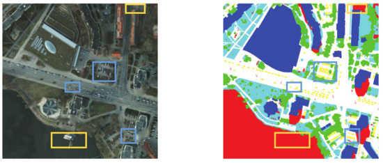  Figure 1. Illustration of Potsdam dataset. The left image is a raw image in Potsdam dataset, and the right image is the corresponding label. Blue boxes mark the tiny objects such as cars, and yellow boxes mark complicated objects such as clutters.
• Due to changes in application scenarios, each data collection needs a certain criterion to judge the category. As shown in yellow boxes in Figure 1, background information includes lake areas, ships and some certain regions in Potsdam dataset. The enormous complexity of remote sensing images causes great difficulty in background understanding.
• Another vexing issue is the unbalanced distribution of each category pixels. In both Potsdam and Vaihingen datasets, the background category is the clutter, and the rest categories including car, tree, building, low vegetation and impervious surface belong to foreground items. The distribution of each object category (including building, background, tree, low vegetation, car and impervious surface) is shown in Figure 2 and Figure 3. In the ISPRS Potsdam dataset, the distribution of foreground and background is out of balance. Background pixels account for 4.70% in the training set (IDs of training images are $02\_10$, $03\_10$, $03\_11$, $03\_12$, $04\_11$, $04\_12$, $05\_10$, $05\_12$, $06\_08$, $06\_09$, $06\_10$, $06\_11$, $06\_12$, $07\_07$, $07\_09$, $07\_11$ and $07\_12$) and 6.48% in the test set (IDs of test images are $02\_11$, $02\_12$, $04\_10$, $05\_11$, $06\_07$, $07\_08$ and $07\_10$). Moreover, all foreground items are not evenly distributed, among which the proportion of car is particularly low due to its small size and haphazard layout. The predicted results (can be observed in section Experimental Results) show that FCN [8] and similar methods cannot explicitly guide recognition of backgrounds due to scarce samples, and FCN and similar methods are likely to misclassify them as foreground pixels.
  

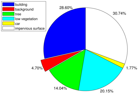  Figure 2. Category distribution of Potsdam training dataset.
  

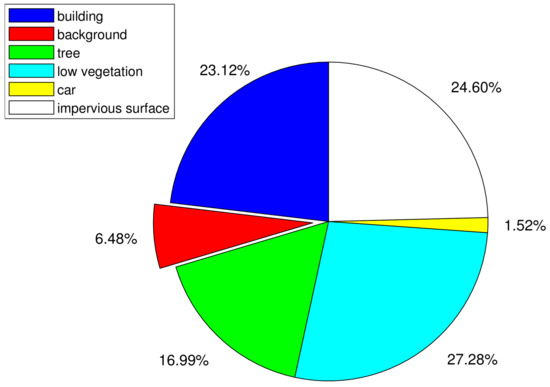  Figure 3. Category distribution of Potsdam test dataset.

In order to improve the reliability of semantic segmentation in remote sensing parsing, our method resorts to the alleviation of the above three problems. The crux of implicit understanding of background information lies in the conflicting fusion of high-level and low-level features, which is a controllable fusion module with adjustable weights that will gradually filter out contradictory information. In order to address the unbalanced distribution of foreground and background pixels, a new optimization strategy combining boundary hard examples mining and the traditional cross-entropy loss function is proposed. At the microscopic level, semantic segmentation indeed divides boundaries of each semantic category, which aids in the identification of tiny objects [14].

In general, the following are our major contributions:

• The principles of semantic segmentation from both a macroscopic and microscopic standpoint are explained. Following these standpoints, our method proposes a controllable fusion module to reduce intra-class inconsistency and an adaptive edge loss function to reduce inter-class confusion based on this idea.
• This paper present a novel semantic segmentation framework for remote sensing parsing that uses the controllable feature module and edge adaptive loss function to improve final performance.
• Our proposed module and loss function can be plugged into mainstream baselines. Extensive experiments on ISPRS Potsdam and ISPRS Vaihingen datasets are carried out to validate their efficiency and attain competitive performance.

2. Related Works

In remote sensing parsing, numerous studies have been reported to focus on semantic segmentation. In this section, relevant advancements in three primary fields will be reviewed, which include semantic segmentation in aerial image analysis, strategies of feature fusion and introduction of edge detection.

2.1. Semantic Segmentation in Aerial Image Analysis

Several previous works have showcased the utility of semantic segmentation in aerial image analysis  [15,16,17,18]. Many related works have progressed in two ways: the designed architecture and the modified mechanism in semantic segmentation. For the sake of algorithm efficiency, they explored fine-grained segmentation with a designed architecture, such as enlarging receptive fields [19] or constructing explicit spatial relations  [20,21,22]. In addition, some works altered the framework of semantic segmentation and successfully applied them in aerial image analysis [23,24,25]. In particular, [26] exploited a new method to avoid the need for costly training data. Their initial generation mechanism was designed to provide more diversified samples with different combinations of objects, directions and locations. Furthermore, a variety of semantic segmentation algorithms was applied to specific task scenarios, such as the change detection of Earth’s surfaces [27], monitoring built-ups [28,29], analyzing urban functional zones [30,31] and aerial reconnaissance by Unmanned Aerial Vehicles [32].

It is admitted that there is a significant and growing demand for up-to-date geospatial data together with methods for the rapid extraction of relevant and useful information that needs to be delivered to stakeholders [33]. This demand for precise geospatial information is constantly growing in order to adapt to the current needs of the world at a global level [34]. Remote sensing parsing is an important task in understanding geospatial data that can provide semantic and localization information cues for interest targets. Remote sensing parsing means analyzing very-high-resolution images, which helps to locate objects at the pixel level and assign them with categorical labels [19,21]. Object-Based Image Analysis (OBIA) has emerged as an effective method of analyzing high spatial resolution images [34]. OBIA is an alternative to a pixel-based method, with the basic analysis unit as image objects instead of individual pixels [35]. Hossain and Chen carried out extensive high-quality research on segmentation for remote sensing parsing and focused on the suitability of specific algorithms [36]. Recently, among the semantic methods, DL has been used in studies [19,37], parsing very high images as it has the capability to treat data as a nested model.

2.2. Strategies of Feature Fusion

The backbone feature fusion modules and head make up the general semantic segmentation paradigm, as shown in Figure 4. The feature fusion module advanced fine-grained segmentation in the initial fully convolutional networks [8]. High-level features contain ample semantic information that helps identify pixel categories, and low-level features contain abundant spatial information, which indicates how pixels are distributed. Feature fusion modules are designed to build relationships between high-level and low-level features. The feature fusion module, in terms of algorithm mechanisms, theoretically guides spatial features with semantic features. Certain refined modules were proposed based on this idea to bridge the gap between high-level and low-level features. Concatenation in channel dimension [38], feature pyramids [39], spatial pyramid poolings [40,41] and non-local modules [42,43] were among the modules that came into effect.

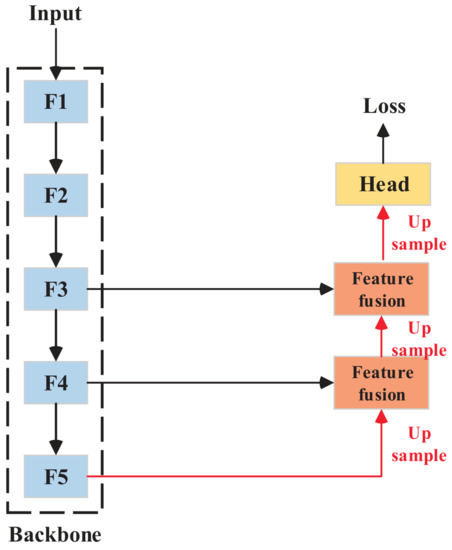
Figure 4. Thg general semantic segmentation paradigm.

2.3. Introduction of Edge Detection

In remote sensing parsing, distinct edge information is critical for remote sensing parsing  [44]. The common methods to supplement edge information include image processing alone  [45,46] and the introduction of extra data (such as Light Detection and Ranging (LiDAR) and digital surface model)  [16]. Automatic extraction of edge information can reduce the data labelling costs and accelerates the development of remote sensing products and services.

The goal of semantic edge detection is to identify distinct inter-class borders [47,48]. Recent works have focused on the fusion of body segmentation and edge preservation [14,49], highlighting the fact that semantic segmentation necessitates object body and edge modeling supervision. As a result, Li et al. [49] developed a unique framework by optimizing body and edge loss in an orthogonal manner, and then combined them as a final loss function. In [48], they held the view that most methods still suffer from intra-class inconsistency and inter-class indistinction. They aimed to acquire features with better homogeneity by using designed architecture to address the problem of intra-class inconsistency. As for the problem of inter-class indistinction, they made supervisory boundary labels from the segmentation ground truth with Canny processing. As demonstrated by Ding et al. [50], Weights in the corner of a square filter usually offer the least information in local feature extraction. Hence, Zheng et al. [19] suggested a cross-like Spatial Pyramid Pooling module. In order to improve learning edge information in DCNNs, they proposed an edge-aware loss, which adds an extra supervised dice-based loss for the edge part.

3. Methodology

3.1. Feature Fusion

The hierarchical backbone network yields feature maps of various sizes, unless otherwise mentioned, the backbone network in our experiments is Resnet-50. Consider feature map $F_i\in {\mathbb{R}}^{H_i\times W_i\times C_i}$ indexed in bottom-to-top order ($H_{i+1}\le H_i$, $W_{i+1}\le W_i$), in which H, W and C are height, width and channel dimension, respectively.

The fusion of multi-level features can be expressed as Equation (1):

$$(F_1,F_2,\dots ,F_i)\to (\widetilde{F_1},\widetilde{F_2},\dots ,\widetilde{F_i}).$$

(1)

where $\widetilde{F_i}$ is the fused output in the i-th layer.

The goal of feature fusions is to integrate semantic information (from top layers) with spatial location information (from bottom layers). As a result, the process essence of feature fusion is to assess the importance of different features and filter out information that is inconsistent.

In mainstream semantic segmentation models, there are several types of feature fusions:

• The spatial pyramid pooling is embedded at the top of backbone networks to encode multi-scale contextual information. PSPNet [41] and Deeplabv3+ [40] built pyramid poolings with different dilation rates in convolutional neural networks.
• In encoder–decoder frame networks, the decoding process uses lateral connections [39] or skip connections [38] to integrate feature information and then outputs predicted probabilities.
• Another type of method computes a weighted sum of the responses at all positions (such as Non-local neural networks [42], CCNet [43]).

Obviously, the fusion strategies described above have not explicitly established the feature correlations and are unable to quantify the importance of each feature. Thus, a controllable feature fusion module is proposed in this paper.

Gating mechanism has been proved to be valid in the evaluation of each feature vector in long-short term memory networks (LSTM) [51]. Inspired by LSTM, the controllable fusion module is depicted in Figure 5, which calculates the weighted sum of all features as the adjustable outputs. In order to explain the whole process, take the controllable fusion module in i-th layer as an example. It can be formulated as follows:

$$\widetilde{F_i}=G_i·F_i+(1-G_i)·\sum _{k\ne 1}{G}_k·F_k,$$

(2)

where the weight factor in i-th layer is $G_i$, and the sum of other layers is factorized by $(1-G_i)$. It is noticeable that the spatial dimensions of other layers are unified as $(H_i,W_i)$ by bilinear interpolation. Furthermore, weight $G_i\in {\mathbb{R}}^{C_i}$ is a vector activated by sigmoid function, and the specific computing process is shown in Equation (3).

$$G_i=\sigma \left(Con{v}_{1\times 1}\left(F_i\right)\right).$$

(3)

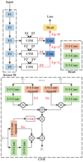
Figure 5. FCN with CFM. The CFM module is applied in F3, F4 and F5 in Resnet-50, and the details of CFM are shown at the bottom. The red lines represent upsampling.

$G_i$ is optimized automatically according to the importance of feature $F_i$. The larger the contribution of $F_i$ to the final prediction, the closer $G_i$ is to one and vice versa.

3.2. Edge Detection

The cross-entropy loss function is a classic loss function in semantic segmentation (shown in Equation (4)):

$$L(y,\widehat{y})=-\frac{1}{N}\sum _{i=1}^N\sum _{k=1}^K[y_{ik}log\left({\widehat{y}}_{ik}\right)+(1-y_{ik})log(1-{\widehat{y}}_{ik})]$$

(4)

where N is the number of total pixels in a batch, K is the total number of categories and y and $\widehat{y}$ represent label and prediction.

Segmentation methods are guided by two criteria: homogeneity within a congener segment and distinction from adjacent segments [33]. Edge-based image segmentation methods attempt to detect edges between regions and then identify segments as regions within these edges. One assumption is that the edge feature aids in pixel location, while the body part containing rich semantic information aids in pixel categorization. The definition and location of edge regions are crucial to guide semantic segmentation with edge information.

Recent research has revealed that purified edge information can help with semantic segmentation. In DFN [14], Canny operator was used to obtain additional edge information labels and a binary loss function was constructed for edge extraction. Gradient mutation of optical image was utilized in some research studies relative to edge perception loss function [19,49]. While the aforementioned works enhanced classification properties, they simply followed the principle that intra-class features (also known as body part) and inter-class features (also known as edge part) are of complete heterology and interact in an orthometric manner. There appears to be an implicit link between intra-class and inter-class features. Assuming that edge-body joint optimization can further improve semantic segmentation, an adaptive edge loss function is proposed.

It is necessary to review the online hard example mining (OHEM) algorithm before elaboration on the proposed adaptive edge loss function. The motivation of OHEM algorithm is to improve the sampling strategy for object-detection algorithms while dealing with extreme distributions of hard and easy cases [52]. The authors proposed the OHEM algorithm for training Fast R-CNN and it proceeded in this manner: At iteration t, the RoI network [53] performs a forward pass using feature maps from the backbone (such as VGG-16) and all RoIs. Top 1% of them were assigned as hard examples after sorting the loss of outputs in descending order (namely take top 1% examples where the network performs worst). When implemented in Fast R-CNN, it computes backward passes only for hard examples in RoIs.

The OHEM loss function could be extended to semantic segmentation frameworks with only modest alterations. Outputs P, which refer to the predicted probability of each category, are sorted in ascending order throughout forward propagation. Threshold probability $\varphi$ is updated according to the preset minimum number of reserved samples $N^{\prime }$ (typically $N^{\prime }$ is 100,000 when patch size is $512\times 512$). Actually, threshold probability $\varphi$ is equal to $P\left[N^{\prime }\right]$, which is the $N^{\prime }$-th value of predicted outputs. Hard examples are those with a probability of less than or equal to $\varphi$. Then, the remaining samples are filled with ignored labels and will not contribute to gradient optimization. Finally, only hard examples contribute to cross-entropy loss.

OHEM loss function is formulated as follows:

$$L(y,\widehat{y})=-\frac{1}{N^{\prime }}\sum _{i=1}^{N^{\prime }}\sum _{k=1}^K[y_{ik}log\left({\widehat{y}}_{ik}\right)+(1-y_{ik})log(1-{\widehat{y}}_{ik})],$$

(5)

where $N^{\prime }$ accounts for the number of pixels participating in practical backpropagation.

Although the OHEM algorithm can mine hard examples in semantic segmentation, the practical findings reveal that a majority of hard examples are dispersed along the boundaries. Different categories can be easily confused with each other due to visual resemblance. Inaccurate classification of pixels adjacent to boundaries is a bottleneck of FCN-likewise methods. The validity of OHEM is due to its ability to identify hard examples allowing for more effective hard-example optimization. Nevertheless, the OHEM loss function treats each pixel equally without identification of edge parts. This feature limits OHEM’s ability to interpret intricate scenes, such as remote sensing photographs. The optimization strategy must also analyze object structures in addition to mining hard examples. Hopefully, segmentation maps contain rich edge clues, which are essentials for semantic edge refinement.

In OHEM loss function, the number of sampled examples $N^{\prime }$ is set in advance, and it will partition all examples into two sections (hard and easy examples). In essence, the OHEM loss function only selects relatively harder samples. Consider the following two extreme scenarios: ① An image patch contains only one single object; ② an image patch comprises a variety of objects. There are many assimilative examples in the first scenario; thus, $N^{\prime }$ shall be reduced to avoid overfitting. In the second scenario, it is difficult to determine an exact category for pixels attached to both sides of the boundary. In this case, $N^{\prime }$ is usually a larger number to ensure sufficient examples for optimization. In the aforementioned cases, the selection of $N^{\prime }$ is fundamentally different, revealing that OHEM cannot precisely suit regardless of how hyperparameter $N^{\prime }$ is selected. Our goal is to design a loss function that can dynamically divide hard and easy examples based on each patch.

The model computes the probability of each label y for a training example x as follows:

$$p\left(k\right|x)=\frac{e^{z_k}}{{\sum }_{i=1}^K{e}^{z_i}},$$

(6)

where k represents the k-th category and $k\in \{1,2,\dots ,K\}$, and $z_i$ is the model’s logits. Assume that for each training example x, the true distribution over labels is $q\left(k\right|x)$ in Equation (7).

$$q\left(k\right|x)=\left\{\begin{array}{cc}1,k=y\hfill & \\ 0,otherwise.\hfill \end{array}\right.$$

(7)

Let us omit the dependence of p and q on example x for the sake of simplicity. Thus, the cross-entropy loss for each example is defined as Equation (8).

$$l=-\sum _{k=1}^{K}q\left(k\right)log\left(p\left(k\right)\right)+(1-q\left(k\right))log(1-p\left(k\right)).$$

(8)

Minimizing this loss function is equivalent to maximizing the expected log-likelihood of the correct label. For a particular example x with label y, the log-likelihood is maximized as $q\left(k\right)={\delta }_{k,y}$ (${\delta }_{k,y}$ is Dirac delta), where the label is selected according to its ground-truth distribution $q\left(k\right)$.

Consider the case of a single ground-truth label y so that $q(k=y)=1$ and $q\left(k\right)=0$ for all $k\ne y$. For a particular example x with label y, the log-likelihood is maximized for $q\left(k\right)={\delta }_{k,y}$, where ${\delta }_{k,y}$ is Dirac delta. The optimization is guided by the cross-entropy loss function, where $z_y$ is substantially larger than $z_k(k\ne y)$.

This strategy, however, may result in over-fitting. If the model learns to assign full probability to the ground-truth label for a particular training example, it is not guaranteed to generalize. Szegedy et al. proposed a regularization mechanism named label-smoothing for a more adaptable optimization [54]. They set a unique distribution over labels $u\left(k\right)$ and a smoothing parameter $\epsilon$ in the label distribution, which were independent of the training example x. For each training example x with ground-truth y, label distribution $q\left(k\right)={\delta }_{k,y}$ was replaced with Equation (9):

$$q^{\prime }\left(k\right)=(1-\epsilon ){\delta }_{k,y}+\epsilon u\left(k\right),$$

(9)

which mixed the original ground-truth distribution $q\left(k\right)$ and the fixed distribution $u\left(k\right)$ with weights $1-\epsilon$ and $\epsilon$, respectively. The distribution of the label k is obtained as follows: First, set it as the ground-truth label $k=y$; then, with probability $\epsilon$, replace k with a sample drawn from the distribution $u\left(k\right)$. They used the uniform distribution as $u\left(k\right)$ so that the label distribution was changed as Equation (10):

$$q^{\prime }\left(k\right)=(1-\epsilon ){\delta }_{k,y}+\frac{\epsilon }{K},$$

(10)

where K is the number of total classes. $\epsilon$ represents the probability of the ground-truth labels being replaced.

In our proposed adaptive edge loss function, the ratio of hard examples to all examples determines $\epsilon$. During actual optimization, a gradient information map using the Laplacian operator (deal with true label distribution) is calculated. Elements with a gradient of 0 are regarded as easy examples, while the other elements are all filled with 1 and are regarded as hard examples (as known as edge parts). Easy examples can only be optimized by cross entropy when constructing the final loss function, while hard examples are input into the adaptive edge loss function for optimization.

The calculation process of our proposed adaptive edge loss function is shown in Algorithm 1, and it can be formulated as follows:

$$\begin{array}{c}\hfill L(y,\widehat{y})=-\frac{1}{N_1}\sum _{i=1}^{N_1}\sum _{k=1}^K[y_{ik}^{easy}log\left({\widehat{y}}_{ik}^{easy}\right)+(1-y_{ik}^{easy})log(1-{\widehat{y}}_{ik}^{easy})]\\ \hfill -\frac{1}{N_2}\sum _{i=1}^{N_2}\sum _{k=1}^K[y{\prime }_{ik}^{hard}log\left({\widehat{y}}_{ik}^{hard}\right)+(1-y{\prime }_{ik}^{hard})log(1-{\widehat{y}}_{ik}^{hard})],\end{array}$$

(11)

where $N_1$ and $N_2$ are the number of easy examples and hard examples, respectively. y is the ground-truth label and $\widehat{y}$ is the predicted probability of the model.

Algorithm 1 Adaptive Edge Loss function

Input:  D: training dataset composed of $x_i,y_i$; K: number of total categories; q: label distribution Output: $\theta$: optimal parameters of the network 1: Initialize parameters of the network according to [55], $N_{hard}\leftarrow 0$, $N_{easy}\leftarrow 0$ 2: for all$x_i,y_i\in$D do 3:     for $k=1$ to $\mathbf{K}$ do 4:         compute predicted probability ${\widehat{y}}_i\left(k\right)=f_{\theta }\left(x_i\right)$ 5:         compute smoothed label distribution $\widehat{q}\left(k\right)=(1-\xi )q\left(k\right)+\frac{\xi }{K}$ 6:         for all pixel $s\in x_i$ do 7:            if Laplace(${\widehat{y}}_s)$ < 0 then 8:                compute loss value for easy examples 9:                $N_1\leftarrow N_1+1$ 10:            end if 11:            if Laplace(${\widehat{y}}_s$) > 0 then 12:                replace $y\left(k\right)$ as $y^{\prime }\left(k\right)$ according to smoothed distribution $\widehat{q}\left(k\right)$ 13:                compute loss value for hard examples 14:                $N_2\leftarrow N_2+1$ 15:            end if 16:         end for 17:     end for 18:     compute final loss value according to Equation (11) 19: end for 20: optimize $\theta$ according to Stochastic Gradient Descent

4. Experimental Results

4.1. Description of Data Sets

The Potsdam and Vaihingen datasets (https://www2.isprs.org/commissions/comm2/wg4/benchmark/ (accessed on 12 December 2013)) are used for benchmarking. The Potsdam dataset consists of 38 high resolution aerial images that cover a total area of 3.42 km${}^2$ and are captured in four channels (near infrared, red, green and blue). All images are 6000 × 6000 pixels in size and are annotated with pixels-level labels of six classes. The spatial resolution is 5 cm, and co-registered DSMs are available as well. In order to train and evaluate networks, 17 RGB images (image IDs: $02\_10$, $03\_10$, $03\_11$, $03\_12$, $04\_11$, $04\_12$, $05\_10$, $05\_12$, $06\_08$, $06\_09$, $06\_10$, $06\_11$, $06\_12$, $07\_07$, $07\_09$, $07\_11$ and $07\_12$) were utilized for training, and the test set was built with remaining RGB images (image IDs: $02\_11$, $02\_12$, $04\_10$, $05\_11$, $06\_07$, $07\_08$ and $07\_10$), which follows the setup in [56,57].

The Vaihingen dataset is composed of 33 aerial images with a spatial resolution of 9 cm that were gathered over a 1.38 km${}^2$ area of Vaihingen. Each image has three bands, corresponding to near infrared, red and green wavelengths with an average size of 2494 × 2064 pixels. Notably, DSMs, which indicate the height of all object surfaces in an image, are also provided as complementary data. Sixteen of the images are manually annotated with pixel-wise labels, and each pixel is classified into one of six land cover classes. Following the setup in [56,58,59], 11 RGB images (image IDs: 1, 3, 5, 7, 13, 17, 21, 23, 26, 32 and 37) were chosen for training, and the remaining five RGB images (image IDs: 11, 15, 28, 30 and 34) were used to test our model.

4.2. Training Details and Metrics

ResNet-50 [60] is chosen as our backbone networks by default. Following the same setting in [37], all models involved were trained with 100 epochs on cropped images. During training, random scale variation (scale range is between 0.5 and 2.0) and horizontal and vertical flip are used for data augmentation. A sliding window striding 256 pixels is applied to crop the image into a fixed size of 512 × 512 for data preprocessing. The mean intersection over union (mIoU) and mean pixel accuracy (MPA) are chosen as the main metrics for evaluation. The baseline for ablation studies is Semantic-FPN [39] with output stride 32.

4.3. Experiments

Extensive experiments concerning the controllable fusion module (hereinafter referred to as CFM) and the adaptive edge loss function (hereinafter referred to as AEL) were conducted.

Ablation experiments with FCN and Deeplabv3 as baseline separately were performed to verify the effectiveness of CFM and AEL. A total of four experiments on Potsdam and Vaihingen datasets were conducted. As shown in Table 1 and Table 2, CFM and AEL can significantly promote FCN like-wise networks. CFM increases by at least 1.148% in mIoU, and AEL increases by at least 2.53% and 0.861% in mIoU and MPA. In the Deeplab like-wise models shown in Table 3 and Table 4, CFM effectively improves mIoU by 2.311%, and AEL effectively improves mIoU by 1.176%.

Table 1. Ablation study of FCN likewise models on Potsdam dataset.

Method	CFM	AEL	mIoU (%)	MPA (%)
Baseline	-	-	69.698	81.223
Baseline	🗸	-	76.811	85.200
Baseline	🗸	🗸	77.959	86.061

CFM means the controllable fusion module. AEL means the adaptive edge loss.

Table 2. Ablation study of Deeplab likewise models on Potsdam dataset.

Method	CFM	AEL	mIoU (%)	MPA (%)
Baseline	-	-	73.340	81.453
Baseline	🗸	-	75.651	82.241
Baseline	🗸	🗸	78.202	86.264

CFM means the controllable fusion module. AEL means the adaptive edge loss.

Table 3. Ablation study of FCN likewise models on Vaihingen dataset.

Method	CFM	AEL	mIoU (%)	MPA (%)
Baseline	-	-	65.782	81.379
Baseline	🗸	-	68.312	82.431
Baseline	🗸	🗸	73.346	84.241

CFM means the controllable fusion module. AEL means the adaptive edge loss.

Table 4. Ablation study of Deeplab likewise models on Vaihingen dataset.

Method	CFM	AEL	mIoU (%)	MPA (%)
Deeplabv3 plus	-	-	68.264	82.942
Deeplabv3 plus	🗸	-	69.440	83.056
Deeplabv3 plus	🗸	🗸	72.368	84.881

CFM means the controllable fusion module. AEL means the adaptive edge loss.

The ablation experimental results showed that both CFM and AEL can play a positive role in the general semantic segmentation framework model, especially in FCN networks.

In addition to the ablation experiments, the hyperparameter selection of the kernel size in AEL was also compared. The kernel size in AEL can only be odd, and the experimental results with kernel size as 3, 5 and 7 were compared respectively. In the following four groups of experiments, mIoU and MPA as evaluation were chosen as metrics shown in Figure 6 and Figure 7. The experimental results showed that the selection of kernel size has limited influence on mIoU and MPA. When the kernel size is 3 and 5, the effect is basically the same. Therefore, the kernel size in AEL is finally set as 5.

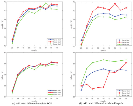
Figure 6. Comparison of different kernels of Adaptive Edge loss on Potsdam dataset. (a) The baseline is FCN. (b) The baseline is Deeplabv3. The metrics are mIoU and MPA.

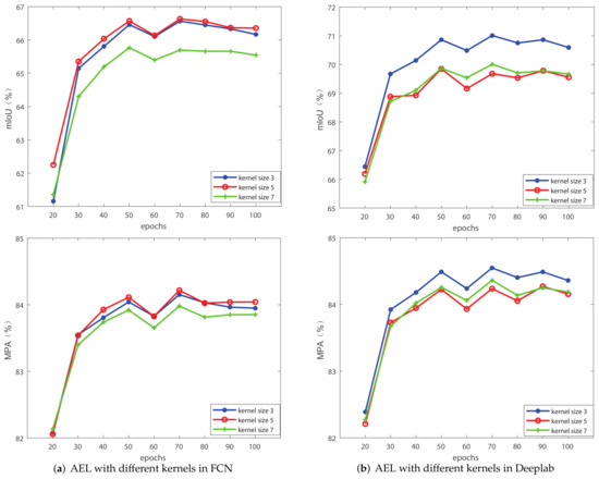
Figure 7. Comparison of different kernels of Adaptive Edge loss on Vaihingen dataset. (a) The baseline is FCN. (b) The baseline is Deeplabv3. The metrics are mIoU and MPA.

Furthermore, CFM is also compared with other general feature fusion modules, including lateral connections in [39], spatial pyramid pooling with dilated convolutions in [40], skip connections in [38], non-local fusion in [42] and semantic flows in [61]. In this group of experiments, the baseline is unified as FCN. The detailed architectures of all fusion modules are depicted in Figure 8, Figure 9 and Figure 10. It is noticeable that Flow warp in [61] referred to [62], but their warping procedure incorporated low-level and high-level features to predict offset fields.

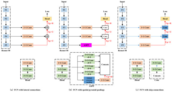
Figure 8. FCN with different fusion modules. (a) FCN with lateral connections. (b) FCN with spatial pyramid poolings. (c) FCN with skip connections. The red lines represent upsampling.

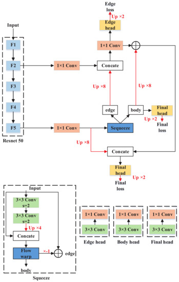
Figure 9. FCN with semantic flows. The red lines represent upsampling.

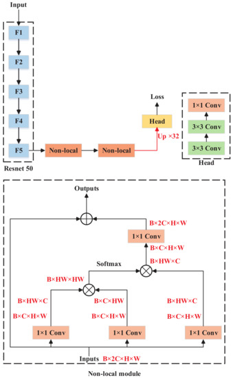
Figure 10. FCN with non-local fusions. B, H, W and C represent batch size, height, width and channel dimension, respectively.

The pixel accuracy of each category (clutter, impervious surface, car, low vegetation, tree and building) is also sorted out in Table 5 and Table 6 in order to comprehensively analyze the performance of each fusion module. In both Potsdam and Vaihingen datasets, the proposed CFM has a significant improvement in mIoU and marginal improvements in MPA. CFM can effectively classify complex categories. In both datasets, the corresponding impervious surface pixel accuracies reach 77.476% and 72.898%, respectively, which are the highest scores among all fusion modules. In parsing clutter pixels, CFM also helps FCN in reaching an almost 2.96% increase in mIoU. Meanwhile, the CFM module can still maintain high accuracy when discriminating small objects (car and tree). Theoretically, CFM constructs a strong attention mechanism, which combines the semantic features of each layer and redistributes weights to correct the prediction results of the model. Thus, it can effectively distinguish the pixels of impervious surface. In addition, its fusion strategy also integrates local and global information; thus, it also promotes the classification of small objects.

Table 5. Results of different fusion modules on Potsdam dataset. CL means clutter. I means impervious surface. CA means car. L means low vegetation. T means tree. B means building. The highest scores are marked in bold.

Method	mIoU (%)	MPA (%)	CL (%)	I (%)	CA (%)	L (%)	T (%)	B (%)
FPN	69.698	81.223	51.013	71.477	69.870	66.361	62.423	78.357
ASPP	71.186	82.141	55.085	73.056	73.530	67.737	61.775	79.834
CONC	69.698	81.223	51.013	71.477	69.870	66.361	62.423	78.357
Decouple	70.671	81.760	52.003	71.900	71.653	67.037	63.289	79.477
Nonlocal	72.857	84.797	54.167	76.131	63.332	71.289	67.294	86.242
CFM	76.811	85.200	54.979	77.476	81.503	71.752	67.613	85.712

CFM means our controllable fusion module.

Table 6. Results of different fusion modules on Vaihingen dataset. CL means clutter. I means impervious surface. CA means car. L means low vegetation. T means tree. B means building. The highest scores are marked in bold.

Method	mIoU (%)	MPA (%)	CL (%)	I (%)	CA (%)	L (%)	T (%)	B (%)
FPN	65.782	81.379	-	71.631	54.503	52.211	70.458	80.108
ASPP	64.357	81.518	-	71.899	45.885	52.458	70.031	81.509
CONC	63.060	81.115	-	71.333	41.602	52.422	69.752	80.193
Decouple	66.155	82.270	-	72.561	50.321	55.878	71.683	80.332
Nonlocal	50.213	74.713	-	63.405	11.482	42.533	61.000	72.645
CFM	68.312	82.431	-	72.898	60.389	55.547	71.255	81.471

CFM means our controllable fusion module.

In the last figure, existing state-of-art models are also represented, which include CCNet [43], Deeplabv3+ [40], PSPNet [41], UNet [38], EANet [19] and Semantic flows (FCN decouple and Deeplab decouple) [49]. All the above networks were retrained on a single 2080-ti with batch size as eight for fairness. The training epoches are 100, and the cropped size is 512. Therefore, their final performance is somewhat different from that in the original paper. Visualization results can be found in Figure 11 and Figure 12.

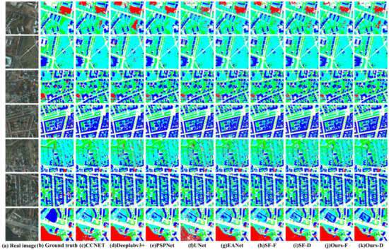
Figure 11. Visualization of all models on Potsdam dataset. (a) Ground truth. (b) Results of CCNet. (c) Results of Deeplabv3+. (d) Results of PSPNet. (e) Results of UNet. (f) Results of EANet. (g) Results of SFNet with FCN. (h) Results of SFNet with Deeplab. (i) Results of our method with FCN. (j) Results of our method with Deeplab.

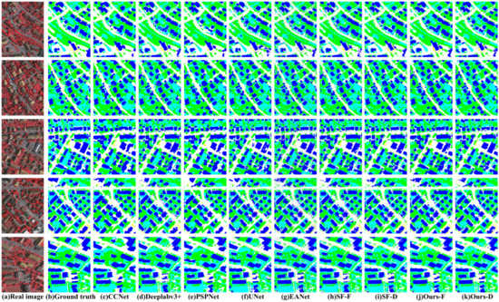
Figure 12. Visualization of all models on Vaihingen dataset. (a) Ground truth. (b) Results of CCNet. (c) Results of Deeplabv3+. (d) Results of PSPNet. (e) Results of UNet. (f) Results of EANet. (g) Results of SFNet with FCN. (h) Results of SFNet with Deeplab. (i) Results of our method with FCN. (j) Results of our method with Deeplab.

The results are shown in Table 7 and Table 8, and some methods are distinguished as two models according to their baselines (SF-F means semantic flows with FCN, SF-D means semantic flows with Deeplab, Ours-F means our proposed methods with FCN, and Ours-D means our proposed methods with Deeplab). In both Potsdam and Vaihingen datasets, FCN and Deeplab embedded with CFM and AEL outperformed other models in terms of mIoU and MPA. CCNet constructs the attention mechanism in the spatial dimension. It can accurately analyze complex categories such as impervious surface. However, it is difficult to identify small objects such as cars and trees. Similar problems can also be found in EANet. There is one possible theoretical explanation for such problems. Their models set strong constraints but failed to establish a clear mapping relationship, which results in the most important and common features but cannot take into account those rare samples.

Table 7. Results of other models on Potsdam dataset. CL means clutter. I means impervious surface. CA means car. L means low vegetation. T means tree. B means building. The highest scores are marked in bold.

Method	mIoU (%)	MPA (%)	CL (%)	I (%)	CA (%)	L (%)	T (%)	B (%)
CCNet	59.073	76.210	46.474	61.563	44.097	60.798	56.834	72.073
Deeplabv3+	73.340	81.453	63.712	72.291	73.264	67.157	60.624	78.363
PSPNet	61.656	78.801	52.140	65.935	43.613	63.461	58.589	76.683
UNet	74.844	83.423	42.027	76.356	79.485	69.498	66.131	82.749
EANet	64.514	80.106	52.378	69.861	50.310	65.593	60.760	76.047
SF-F	70.671	81.760	52.003	71.900	71.653	67.037	63.289	79.477
SF-D	77.079	85.404	55.872	77.879	81.732	71.787	67.977	86.018
Ours-F	77.959	86.061	54.293	79.133	81.602	72.891	68.143	88.025
Ours-D	78.202	86.264	68.193	79.058	79.939	81.775	72.884	88.219

Table 8. Results of other models on Vaihingen dataset. CL means clutter. I means impervious surface. CA means car. L means low vegetation. T means tree. B means building. The highest scores are marked in bold.

Method	mIoU (%)	MPA (%)	CL (%)	I (%)	CA (%)	L (%)	T (%)	B (%)
CCNet	51.843	74.669	-	63.049	18.980	43.439	60.627	73.118
Deeplabv3+	68.264	82.942	-	73.700	57.164	56.752	72.267	81.435
PSPNet	51.325	75.513	-	64.519	11.999	43.837	61.475	74.793
UNet	68.001	83.519	-	75.191	51.941	57.322	72.134	83.416
EANet	64.964	80.448	-	69.814	55.732	54.652	67.983	76.639
SF-F	66.155	82.270	-	72.561	50.321	55.878	71.683	80.332
SF-D	72.274	84.750	-	77.514	65.860	60.211	72.838	86.046
Ours-F	73.346	84.241	-	77.504	62.148	59.571	73.849	86.658
Ours-D	72.368	84.881	-	77.388	66.064	59.542	73.326	85.518

Establishing an explicit fusion relationship between edge features and body features can indeed advance remote sensing parsing. Semantic flows constructed flow-warp procedure in order to optimize edge loss and body loss; hence, it can achieve clear accuracy leadings on both datasets. Similarly, our proposed scheme improves the feature fusion process and edge-body loss optimization. It should be noted that these two strategies are fundamentally different. During the process of feature fusion, the CFM proposed in this paper actually fuses all features and then carries out self calibration, while the strategy of semantic flows is to extract edge and subject features in a decoupled manner. When analyzing complex and changeable impervious surfaces, the models with CFM and AEL have achieved leading accuracy. When analyzing small targets, the model also achieves a significant improvement.

Only the controllable fusion module (CFM) proposed in this paper is involved with inference. Therefore, four groups of experimental results are recorded in Table 9. Compared with the baselines (FCN and Deeplabv3 plus), the forward inference time of CFM increased by 15 ms and 12 ms. In view of its gain in mIoU and MPA, CFM is still cost-effective feature fusion module.

Table 9. Inference time of our methods.

Method	Inference Time (ms)
FCN	150
FCN + CFM	165 ↑(15)
Deeplabv3 plus	116
Deeplabv3 plus + CFM	128 ↑(12)

5. Discussion

The experimental results indicate that our proposed method has three advantages over other algorithms. First, our proposed controllable fusion module and adaptive edge loss function can be plugged into general baselines (such as FCN and Deeplabv3) with minimal modifications. The final evaluation metrics prove that our modified modules can significantly improve the baselines. Second, our modified networks can effectively filter out distractors. In Potsdam and Vaihingen datasets, categories such as clutters and buildings have high semantic complexity. During upsampling, our proposed controllable fusion modules adjust features at all levels and automatically determine weight values for all features according to their importance. In the final weighted fusion, our modified networks realize valid recognition for different categories. Third, our proposed method is capable of dealing with tiny objects (such cars and trees). Inspired by edge detection, our proposed adaptive edge loss function further mines difficult samples in edge information, which is helpful for identifying small targets. In short, our proposed method has a powerful feature fusion ability and detailed recovery capability for high-resolution remote sensing images. Our method achieves competitive results, but further work on remote sensing parsing still needs to be conducted.

6. Conclusions

In this study, a controllable fusion module (CFM) and an adaptive edge loss (AEL) are proposed to solve problems in remote sensing parsing. Currently, parsing algorithms based on semantic segmentation are trapped in three aspects including frequent neglect of small distributed objects, high complexity of category understanding and unbalanced distribution of categories. Our proposed CFM helps to construct an explicit relationship between all-level features, which achieves 7.113% and 2.53% mIoU improvement in Potsdam and Vaihingen datasets, respectively. AEL can dynamically optimize hard samples in edge pixels and simultaneously optimize body pixels. Results of ablation experiments reveal that AEL achieves up to 4.862% and 7.564% mIoU improvement in Potsdam and Vaihingen datasets. The strategies described above improve semantic segmentation models in a coupled manner. The proposed CFM and AEL can be embedded into mainstream baselines such as FCN and Deeplabv3, and the final results show that our methods achieve best performances of 78.202% and 73.346% mIoU in Potsdam and Vaihingen datasets.

References

- Ohki, M.; Shimada, M. Large-area land use and land cover classification with quad, compact, and dual polarization SAR data by PALSAR-2. IEEE Trans. Geosci. Remote Sens. 2018, 56, 5550–5557. [Google Scholar] [CrossRef]
- Su, H.; Yao, W.; Wu, Z.; Zheng, P.; Du, Q. Kernel low-rank representation with elastic net for China coastal wetland land cover classification using GF-5 hyperspectral imagery. ISPRS J. Photogramm. Remote Sens. 2021, 171, 238–252. [Google Scholar] [CrossRef]
- Luo, X.; Tong, X.; Pan, H. Integrating Multiresolution and Multitemporal Sentinel-2 Imagery for Land-Cover Mapping in the Xiongan New Area, China. IEEE Trans. Geosci. Remote Sens. 2020, 59, 1029–1040. [Google Scholar] [CrossRef]
- Xu, F.; Somers, B. Unmixing-based Sentinel-2 downscaling for urban land cover mapping. ISPRS J. Photogramm. Remote Sens. 2021, 171, 133–154. [Google Scholar] [CrossRef]
- Marconcini, M.; Fernández-Prieto, D.; Buchholz, T. Targeted land-cover classification. IEEE Trans. Geosci. Remote Sens. 2013, 52, 4173–4193. [Google Scholar] [CrossRef]
- Antropov, O.; Rauste, Y.; Astola, H.; Praks, J.; Häme, T.; Hallikainen, M.T. Land cover and soil type mapping from spaceborne PolSAR data at L-band with probabilistic neural network. IEEE Trans. Geosci. Remote Sens. 2013, 52, 5256–5270. [Google Scholar] [CrossRef]
- Song, L.; Xia, M.; Jin, J.; Qian, M.; Zhang, Y. SUACDNet: Attentional change detection network based on siamese U-shaped structure. Int. J. Appl. Earth Obs. Geoinf. 2021, 105, 102597. [Google Scholar] [CrossRef]
- Long, J.; Shelhamer, E.; Darrell, T. Fully convolutional networks for semantic segmentation. In Proceedings of the IEEE Conference on Computer Vision and Pattern Recognition, Boston, MA, USA, 7–12 June 2015; pp. 3431–3440. [Google Scholar]
- Siam, M.; Gamal, M.; Abdel-Razek, M.; Yogamani, S.; Jagersand, M.; Zhang, H. A comparative study of real-time semantic segmentation for autonomous driving. In Proceedings of the IEEE Conference on Computer Vision and Pattern Recognition Workshops, Salt Lake City, UT, USA, 18–22 June 2018; pp. 587–597. [Google Scholar]
- Tang, H.; Xu, D.; Yan, Y.; Torr, P.H.; Sebe, N. Local class-specific and global image-level generative adversarial networks for semantic-guided scene generation. In Proceedings of the IEEE/CVF Conference on Computer Vision and Pattern Recognition, Seattle, WA, USA, 13–19 June 2020; pp. 7870–7879. [Google Scholar]
- Ding, L.; Zhang, J.; Bruzzone, L. Semantic segmentation of large-size VHR remote sensing images using a two-stage multiscale training architecture. IEEE Trans. Geosci. Remote Sens. 2020, 58, 5367–5376. [Google Scholar] [CrossRef]
- Xia, M.; Zhang, X.; Liu, W.; Weng, L.; Xu, Y. Multi-Stage Feature Constraints Learning for Age Estimation. IEEE Trans. Inform. Forensics Secur. 2020, 15, 2417–2428. [Google Scholar] [CrossRef]
- He, A.; Luo, C.; Tian, X.; Zeng, W. A twofold siamese network for real-time object tracking. In Proceedings of the IEEE Conference on Computer Vision and Pattern Recognition, Salt Lake City, UT, USA, 18–23 June 2018; pp. 4834–4843. [Google Scholar]
- Yu, C.; Wang, J.; Peng, C.; Gao, C.; Yu, G.; Sang, N. Learning a discriminative feature network for semantic segmentation. In Proceedings of the IEEE Conference on Computer Vision and Pattern Recognition, Salt Lake City, UT, USA, 18 June 2018; pp. 1857–1866. [Google Scholar]
- Kaiser, P.; Wegner, J.D.; Lucchi, A.; Jaggi, M.; Hofmann, T.; Schindler, K. Learning aerial image segmentation from online maps. IEEE Trans. Geosci. Remote Sens. 2017, 55, 6054–6068. [Google Scholar] [CrossRef]
- Marmanis, D.; Schindler, K.; Wegner, J.D.; Galliani, S.; Datcu, M.; Stilla, U. Classification with an edge: Improving semantic image segmentation with boundary detection. ISPRS J. Photogramm. Remote Sens. 2018, 135, 158–172. [Google Scholar] [CrossRef] [Green Version]
- Qu, Y.; Xia, M.; Zhang, Y. Strip pooling channel spatial attention network for the segmentation of cloud and cloud shadow. Comput. Geosci. 2021, 157, 104940. [Google Scholar] [CrossRef]
- Chen, B.; Xia, M.; Huang, J. MFANet: A Multi-Level Feature Aggregation Network for Semantic Segmentation of Land Cover. Remote Sens. 2021, 13, 731. [Google Scholar] [CrossRef]
- Zheng, X.; Huan, L.; Xia, G.S.; Gong, J. Parsing very high resolution urban scene images by learning deep ConvNets with edge-aware loss. ISPRS J. Photogramm. Remote Sens. 2020, 170, 15–28. [Google Scholar] [CrossRef]
- Yang, X.; Li, S.; Chen, Z.; Chanussot, J.; Jia, X.; Zhang, B.; Li, B.; Chen, P. An attention-fused network for semantic segmentation of very-high-resolution remote sensing imagery. ISPRS J. Photogramm. Remote Sens. 2021, 177, 238–262. [Google Scholar] [CrossRef]
- Diakogiannis, F.I.; Waldner, F.; Caccetta, P.; Wu, C. ResUNet-a: A deep learning framework for semantic segmentation of remotely sensed data. ISPRS J. Photogramm. Remote Sens. 2020, 162, 94–114. [Google Scholar] [CrossRef] [Green Version]
- Mou, L.; Hua, Y.; Zhu, X.X. Relation matters: Relational context-aware fully convolutional network for semantic segmentation of high-resolution aerial images. IEEE Trans. Geosci. Remote Sens. 2020, 58, 7557–7569. [Google Scholar] [CrossRef]
- Sun, Y.; Zhang, X.; Xin, Q.; Huang, J. Developing a multi-filter convolutional neural network for semantic segmentation using high-resolution aerial imagery and LiDAR data. ISPRS J. Photogramm. Remote Sens. 2018, 143, 3–14. [Google Scholar] [CrossRef]
- Li, Y.; Shi, T.; Zhang, Y.; Chen, W.; Wang, Z.; Li, H. Learning deep semantic segmentation network under multiple weakly-supervised constraints for cross-domain remote sensing image semantic segmentation. ISPRS J. Photogramm. Remote Sens. 2021, 175, 20–33. [Google Scholar] [CrossRef]
- Feng, Y.; Sun, X.; Diao, W.; Li, J.; Gao, X.; Fu, K. Continual Learning With Structured Inheritance for Semantic Segmentation in Aerial Imagery. IEEE Trans. Geosci. Remote Sens. 2021, 60, 5607017. [Google Scholar] [CrossRef]
- Pan, X.; Zhao, J.; Xu, J. Conditional Generative Adversarial Network-Based Training Sample Set Improvement Model for the Semantic Segmentation of High-Resolution Remote Sensing Images. IEEE Trans. Geosci. Remote Sens. 2020, 59, 7854–7870. [Google Scholar] [CrossRef]
- Qian, J.; Xia, M.; Zhang, Y.; Liu, J.; Xu, Y. TCDNet: Trilateral Change Detection Network for Google Earth Image. Remote Sens. 2020, 12, 2669. [Google Scholar] [CrossRef]
- Wu, F.; Wang, C.; Zhang, H.; Li, J.; Li, L.; Chen, W.; Zhang, B. Built-up area mapping in China from GF-3 SAR imagery based on the framework of deep learning. Remote Sens. Environ. 2021, 262, 112515. [Google Scholar] [CrossRef]
- Chen, J.; Qiu, X.; Ding, C.; Wu, Y. CVCMFF Net: Complex-Valued Convolutional and Multifeature Fusion Network for Building Semantic Segmentation of InSAR Images. IEEE Trans. Geosci. Remote Sens. 2021, 60, 5205714. [Google Scholar] [CrossRef]
- Du, S.; Du, S.; Liu, B.; Zhang, X. Mapping large-scale and fine-grained urban functional zones from VHR images using a multi-scale semantic segmentation network and object based approach. Remote Sens. Environ. 2021, 261, 112480. [Google Scholar] [CrossRef]
- Luo, H.; Chen, C.; Fang, L.; Khoshelham, K.; Shen, G. Ms-rrfsegnet: Multiscale regional relation feature segmentation network for semantic segmentation of urban scene point clouds. IEEE Trans. Geosci. Remote Sens. 2020, 58, 8301–8315. [Google Scholar] [CrossRef]
- Masouleh, M.K.; Shah-Hosseini, R. Development and evaluation of a deep learning model for real-time ground vehicle semantic segmentation from UAV-based thermal infrared imagery. ISPRS J. Photogramm. Remote Sens. 2019, 155, 172–186. [Google Scholar] [CrossRef]
- Kotaridis, I.; Lazaridou, M. Remote sensing image segmentation advances: A meta-analysis. ISPRS J. Photogramm. Remote Sens. 2021, 173, 309–322. [Google Scholar] [CrossRef]
- Lang, S. Object-based image analysis for remote sensing applications: Modeling reality–dealing with complexity. In Object-Based Image Analysis; Springer: Berlin/Heidelberg, Germany, 2008; pp. 3–27. [Google Scholar]
- Castilla, G.; Hay, G.G.; Ruiz-Gallardo, J.R. Size-constrained region merging (SCRM). Photogramm. Eng. Remote Sens. 2008, 74, 409–419. [Google Scholar] [CrossRef]
- Hossain, M.D.; Chen, D. Segmentation for Object-Based Image Analysis (OBIA): A review of algorithms and challenges from remote sensing perspective. ISPRS J. Photogramm. Remote Sens. 2019, 150, 115–134. [Google Scholar] [CrossRef]
- Li, X.; He, H.; Li, X.; Li, D.; Cheng, G.; Shi, J.; Weng, L.; Tong, Y.; Lin, Z. PointFlow: Flowing Semantics Through Points for Aerial Image Segmentation. In Proceedings of the IEEE/CVF Conference on Computer Vision and Pattern Recognition, Online Conference, 19 June 2021; pp. 4217–4226. [Google Scholar]
- Ronneberger, O.; Fischer, P.; Brox, T. U-net: Convolutional networks for biomedical image segmentation. In Proceedings of the International Conference on Medical Image Computing and Computer-Assisted Intervention, Boston, MA, USA, 8 June 2015; Springer: Berlin/Heidelberg, Germany, 2015; pp. 234–241. [Google Scholar]
- Kirillov, A.; Girshick, R.B.; He, K.; Dollár, P. Panoptic Feature Pyramid Networks. In Proceedings of the IEEE Conference on Computer Vision and Pattern Recognition, Long Beach, CA, USA, 16 June 2019; pp. 6399–6408. [Google Scholar]
- Chen, L.C.; Zhu, Y.; Papandreou, G.; Schroff, F.; Adam, H. Encoder-decoder with atrous separable convolution for semantic image segmentation. In Proceedings of the European Conference on Computer Vision (ECCV), Munich, Germany, 8 September 2018; pp. 801–818. [Google Scholar]
- Zhao, H.; Shi, J.; Qi, X.; Wang, X.; Jia, J. Pyramid scene parsing network. In Proceedings of the IEEE Conference on Computer Vision and Pattern Recognition, Honolulu, HI, USA, 22 July 2017; pp. 2881–2890. [Google Scholar]
- Wang, X.; Girshick, R.; Gupta, A.; He, K. Non-local neural networks. In Proceedings of the IEEE Conference on Computer Vision and Pattern Recognition, Salt Lake City, UT, USA, 18 June 2018; pp. 7794–7803. [Google Scholar]
- Huang, Z.; Wang, X.; Huang, L.; Huang, C.; Wei, Y.; Liu, W. Ccnet: Criss-cross attention for semantic segmentation. In Proceedings of the IEEE/CVF International Conference on Computer Vision, Long Beach, CA, USA, 16 June 2019; pp. 603–612. [Google Scholar]
- Li, A.; Jiao, L.; Zhu, H.; Li, L.; Liu, F. Multitask Semantic Boundary Awareness Network for Remote Sensing Image Segmentation. IEEE Trans. Geosci. Remote Sens. 2021. [Google Scholar] [CrossRef]
- Shi, Y.; Li, Q.; Zhu, X.X. Building segmentation through a gated graph convolutional neural network with deep structured feature embedding. ISPRS J. Photogramm. Remote Sens. 2020, 159, 184–197. [Google Scholar] [CrossRef] [PubMed]
- Waldner, F.; Diakogiannis, F.I. Deep learning on edge: Extracting field boundaries from satellite images with a convolutional neural network. Remote Sens. Environ. 2020, 245, 111741. [Google Scholar] [CrossRef]
- Yu, Z.; Feng, C.; Liu, M.; Ramalingam, S. CASENet: Deep Category-Aware Semantic Edge Detection. In Proceedings of the IEEE Conference on Computer Vision and Pattern Recognition, Honolulu, HI, USA, 22 July 2017; pp. 1761–1770. [Google Scholar]
- Liu, Y.; Cheng, M.M.; Hu, X.; Wang, K.; Bai, X. Richer convolutional features for edge detection. In Proceedings of the IEEE Conference on Computer Vision and Pattern Recognition, Honolulu, Hawaii, 22 July 2017; pp. 3000–3009. [Google Scholar]
- Li, X.; Li, X.; Zhang, L.; Cheng, G.; Shi, J.; Lin, Z.; Tan, S.; Tong, Y. Improving Semantic Segmentation via Decoupled Body and Edge Supervision. In Proceedings of the Computer Vision—ECCV 2020—16th European Conference, Glasgow, UK, 23–28 August 2020; Part XVII. Springer: Berlin/Heidelberg, Germany, 2020; Volume 12362, pp. 435–452. [Google Scholar]
- Ding, H.; Jiang, X.; Liu, A.Q.; Magnenat-Thalmann, N.; Wang, G. Boundary-Aware Feature Propagation for Scene Segmentation. In Proceedings of the IEEE/CVF International Conference on Computer Vision, Long Beach, CA, USA, 16 June 2019; pp. 6818–6828. [Google Scholar]
- Hochreiter, S.; Schmidhuber, J. Long Short-Term Memory. Neural Comput. 1997, 9, 1735–1780. [Google Scholar] [CrossRef]
- Shrivastava, A.; Gupta, A.; Girshick, R. Training region-based object detectors with online hard example mining. In Proceedings of the IEEE Conference on Computer Vision and Pattern Recognition, Las Vegas, NV, USA, 26 June 2016; pp. 761–769. [Google Scholar]
- Girshick, R. Fast r-cnn. In Proceedings of the IEEE International Conference on Computer Vision, Boston, MA, USA, 8 June 2015; pp. 1440–1448. [Google Scholar]
- Szegedy, C.; Vanhoucke, V.; Ioffe, S.; Shlens, J.; Wojna, Z. Rethinking the inception architecture for computer vision. In Proceedings of the IEEE Conference on Computer Vision and Pattern Recognition, Las Vegas, NV, USA, 26 June 2016; pp. 2818–2826. [Google Scholar]
- He, K.; Zhang, X.; Ren, S.; Sun, J. Delving deep into rectifiers: Surpassing human-level performance on imagenet classification. In Proceedings of the IEEE International Conference on Computer Vision, Boston, MA, USA, 8 June 2015; pp. 1026–1034. [Google Scholar]
- Maggiori, E.; Tarabalka, Y.; Charpiat, G.; Alliez, P. High-resolution aerial image labeling with convolutional neural networks. IEEE Trans. Geosci. Remote Sens. 2017, 55, 7092–7103. [Google Scholar] [CrossRef] [Green Version]
- Sherrah, J. Fully Convolutional Networks for Dense Semantic Labelling of High-Resolution Aerial Imagery. arXiv 2016, arXiv:1606.02585. [Google Scholar]
- Volpi, M.; Tuia, D. Dense Semantic Labeling of Subdecimeter Resolution Images With Convolutional Neural Networks. IEEE Trans. Geosci. Remote Sens. 2017, 55, 881–893. [Google Scholar] [CrossRef] [Green Version]
- Marcos, D.; Volpi, M.; Kellenberger, B.; Tuia, D. Land cover mapping at very high resolution with rotation equivariant CNNs: Towards small yet accurate models. ISPRS J. Photogramm. Remote Sens. 2018, 145, 96–107. [Google Scholar] [CrossRef] [Green Version]
- He, K.; Zhang, X.; Ren, S.; Sun, J. Deep residual learning for image recognition. In Proceedings of the IEEE Conference on Computer Vision and Pattern Recognition, Las Vegas, NV, USA, 26 June 2016; pp. 770–778. [Google Scholar]
- Li, X.; You, A.; Zhu, Z.; Zhao, H.; Yang, M.; Yang, K.; Tan, S.; Tong, Y. Semantic flow for fast and accurate scene parsing. In Proceedings of the European Conference on Computer Vision; Springer: Berlin/Heidelberg, Germany, 2020; pp. 775–793. [Google Scholar]
- Dai, J.; Qi, H.; Xiong, Y.; Li, Y.; Zhang, G.; Hu, H.; Wei, Y. Deformable Convolutional Networks. In Proceedings of the IEEE International Conference on Computer Vision, ICCV 2017, Venice, Italy, 22–29 October 2017; pp. 764–773. [Google Scholar]
Publisher’s Note: MDPI stays neutral with regard to jurisdictional claims in published maps and institutional affiliations. |
© 2022 by the authors. Licensee MDPI, Basel, Switzerland. This article is an open access article distributed under the terms and conditions of the Creative Commons Attribution (CC BY) license (https://creativecommons.org/licenses/by/4.0/).