1. Introduction
Polarimetric synthetic aperture radar (PolSAR), a kind of multichannel synthetic aperture radar (SAR), has four channels, HH, HV, VH, and VH, which are formed according to the vertical and horizontal transmission and reception of electromagnetic waves. The polarization of back-scattering waves changes after being reflected by the targets; then, the polarimetric sensors provide more information to describe the land surface structure, land covers, geometrical structures, etc. The targets on the ground can be described using a so-called scattering coefficient that can represent the interaction of an electromagnetic wave with the targets [
1].
Compared with optical radar, PolSAR data can actively obtain more information on land cover by alternately transmitting and receiving electromagnetic waves. After obtaining more comprehensive backscattering information, this multichannel sensor can describe land covers from many perspectives, such as color and texture in pseudo-color images, components in coherent or incoherent target decomposition algorithms and parameters, and coefficients in back-scattering matrices [
2,
3,
4]. Recently, lots of researchers have devoted themselves to PolSAR land cover classification, segmentation, clustering, or other pixel-level tasks [
5,
6,
7].
With the development of radar imaging techniques, more sensors with high precision and polarimetric channels (such as ALOS-2, GF3, and TerraSAR-X) have been launched. The continual launching of remote sensing satellites produces a monotonically increasing amount of data. These satellites provide large amounts of data for learning and produce more high-resolution images to extend the research field from pixel-level to target-level and scene-level tasks [
8]. Limited by the difficulty of accessing the full polarimetric data, they lag behind the development of PolSAR image scene classification. However, there is still a huge potential for PolSAR data to deal with scene-level data understanding [
9].
PolSAR data have multimodal features in different representation spaces to create a comprehensive description of the targets. The eigenvalue decomposition H/A/
with Wishart-based distance was adopted for unsupervised classification in the early days [
10]. Furthermore, target decomposition theorems (including model-, eigenvector-, or eigenvalue-based incoherent and coherent decompositions) are exploited to provide physical interpretations of the targets, in which some feature extraction methods are proposed to describe the PolSAR samples as much as possible [
1,
11,
12,
13,
14,
15,
16]. In the literature [
2], texture is first investigated as a valuable resource for PolSAR classification, and some image feature extraction techniques (such as the gray-level co-occurrence matrix [
17,
18], Gabor wavelets [
19,
20], fractal features [
21,
22], etc.) are analyzed to represent the pixels in the image.
Overall, with those multimodal features, one still needs to analyze the properties of those features and make a comprehensive fusion technique for the corresponding tasks. Current existing multi-view space clustering (MSC) methods open a new avenue for combining those features, which maintains consistency among different feature spaces in a clustering structure [
23]. Some low-rank or sparse constraints are exploited to construct the affinity matrix and encourage the sparsity and low-rankness of the solution [
24]. Especially for image-level tasks, an image can be represented by a tensor; then, the tensor-based MSC method is designed, which may also be constrained by a variety of regularization terms [
25]. PolSAR data are represented by features in multiple spaces, and PolSAR images can be formulated as tensors. Therefore, determining how to make full use of those PolSAR tensorial forms and exploit the underlying properties in a multimodal features space is very significant for PolSAR data interpretation.
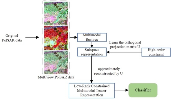
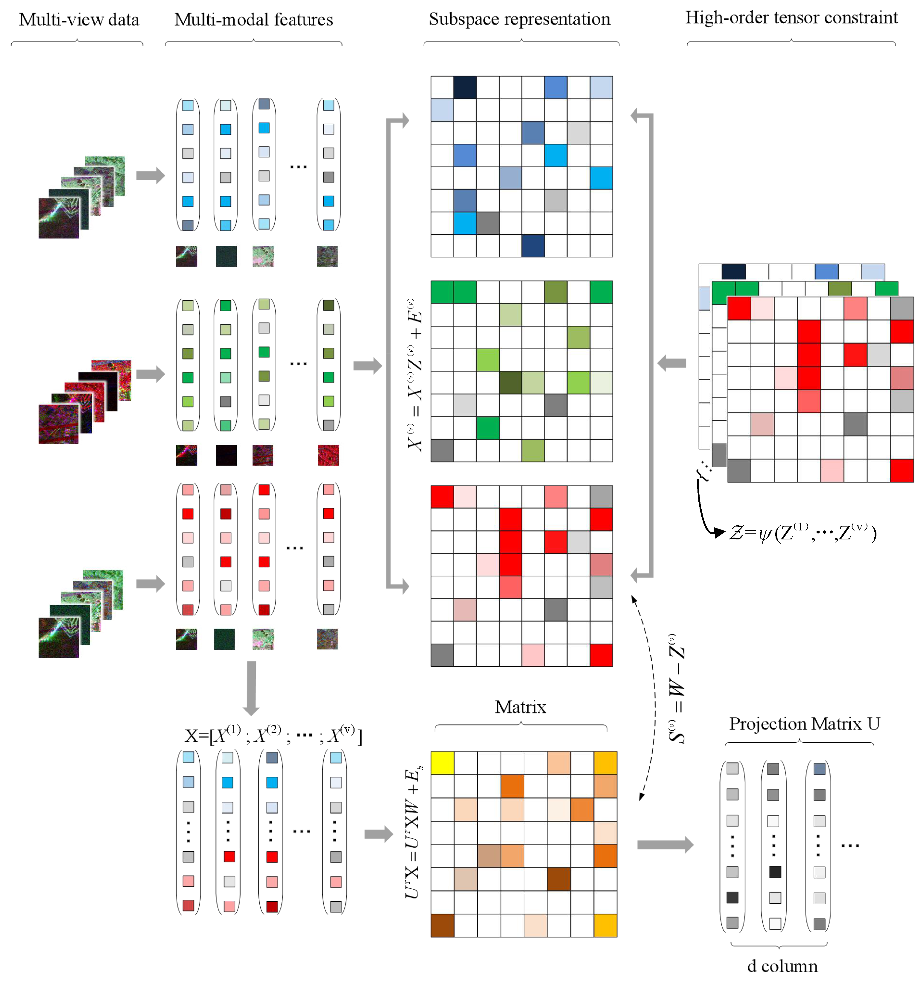
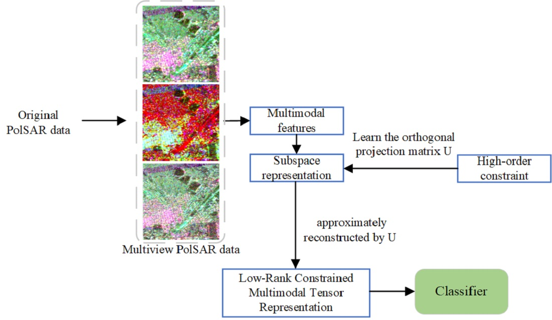
Inspired by multi-view space clustering algorithms, a novel low-rank constrained multimodal tensor representation method (LR-MTR) is proposed to combine multiple features in PolSAR data for scene classification. Different from the most prevalent existing tensor-based PolSAR or hyperspectral land cover classification methods regarding each sample as a tensor [
26,
27,
28,
29,
30], the proposed method constructs all the representation matrices in different spaces as a tensor, as shown in
Figure 1. Furthermore, the high-order representation tensor is constrained by a low-rank norm to model the cross-information from multiple different subspaces. It reduces the unnecessary information of subspace representations in calculations and captures the complementary information among those multiple features. A projection matrix is also calculated by minimizing the difference between all the cascaded features and the features in the corresponding space, which will reduce the difference between the global and single feature spaces. The learned projection matrix can effectively solve the out-of-sample problem in a large-scale data set. Two typical matrices are alternately updated in the optimization: the affinity matrices learned from the multimodal PolSAR data samples and the projection matrix calculated by the representation tensor. Finally, to produce the final results, K-nearest neighbor (KNN) and support vector machine (SVM) classifiers are applied. To solve the complex minimization problem, an augmented Lagrangian alternating direction minimization (AL-ADM) [
31,
32] algorithm has been applied.
This study has four contributions, as follows:
(1) A new dimension reduction algorithm is introduced. This new algorithm integrates the original multimodal features and extracts an eigenvalue decomposition-based projection matrix. We develop a new framework for image feature extraction. Our method can search the optimal projection matrix and optimal subspace simultaneously.
(2) PolSAR coherency/covariance/scattering matrices and various polarimetric target decomposition can be utilized to describe PolSAR data in multimodal feature spaces. To derive a comprehensive representation, the pseudo-color images from Freeman, Cloude, and Pauli are provided to represent the data. This paper describes PolSAR data via multimodal images and tests the visual information via some efficiency texture extraction methods.
(3) To obtain the correlation among the underlying multimodal data and to congregate those features, LR-MTR regards all the subspace features as high-order, so it can be seen as a tensor. With the constraint of a low-rank term, the tensor models the cross-information and obtains representation matrices in the multimodal subspace. LR-MTR reduces the redundancy of the learned subspace representation. Meanwhile, the LR-MTR algorithm also performs with better accuracy on PolSAR scene classification.
(4) Due to the difficulty of accessing PolSAR data, studies in PolSAR image scene classification are relatively rare. To effectively process and investigate this field, we use the semantic information to label images according to the actual land cover situation. Two new full-polarization PolSAR data sets covering Shanghai and Tokyo, produced by ALOS-2, are exploited to build scene classification data.
On the algorithm level, this method introduces a novel multimodal tensor representation method. It does not directly represent samples in the data domain, but constructs a representation tensor under a new tensor low-rank constraint. It learns a representative projection matrix to reduce the redundant information and projects all the features from different modalities into the representation space. Furthermore, the fused features are obtained for the subsequent PolSAR scene classification.
We organize the remaining parts of this study as follows.
Section 2 introduces the related works. In
Section 3, we introduce the motivation of our algorithm, the theory and methodology of the proposed algorithm, and the optimal solution. In
Section 4, experiments are undertaken to show the efficiency of our algorithm. The experimental analysis and visualization results are used to present our data sets. In
Section 5, the conclusion is provided.
3. LR-MTR
In this section, we introduce the motivation of LR-MTR, the specific algorithm, and the optimization.
represent multi-view features data collection. LR-MTR calculates the projection matrix
U by minimizing the difference between the whole cascaded data set and the features in the corresponding space and combines the subspace representations features into a low-rank tensor
Z. The projection matrix is used for linear dimension reduction. LR-MTR utilizes the tensor to model the high-order correlations from multimodal data and obtains a series of representation matrices in the multimodal subspace. The overview of LR-MTR is shown in
Figure 1.
3.1. The Motivation of the Method
Most of the existing representative linear dimension reduction methods mainly use geometric, sample metric, or class-specific structures to calculate the similarity of samples and learn a projection matrix for feature extraction. For example, the well-known locality preserving projection (LPP) constructs a similarity graph and retains the local relationships among the data, neighbor preserving embedding (NPE) uses the same thought, and linear discriminant analysis (LDA) employs label information to search for a linear combination of features from two or more known categories. These approaches all process the cascaded features without considering the consistency and independence of the multi-view features from one sample. In the real world, one modal feature is not guaranteed to effectively describe a sample, especially for remote sensing data. The PolSAR is a multi-channel radar sensor and can be represented by some typical modalities, such as color and textures in pseudo-images, coefficients in incoherent/coherent target decompositions, and free parameters in scattering matrices. PolSAR scene classification, taking each image as one sample, can make full use of the information from the PolSAR image, including not only the spatial knowledge, but also the redundant features provided by PolSAR multi-channel descriptors.
Thus, it is urgent to simultaneously exploit the multimodal PolSAR features for data processing. In different representation spaces, PolSAR data have multimodal features to create a comprehensive description for the targets, which can be directly constructed into a high-order tensor. It will seek the spatial information from multi-view data and correlate multimodal features. These high-order tensor samples can extend the linear dimension reduction algorithms to tensor forms, such as tensor locality preserving projection (TLPP) or tensor neighbor preserving embedding (TNPE), but this also results in the huge computation of calculating the tensor similarities and constructing tensor graphs. We try to use representation matrices from multi-view subspaces to construct a tensor that can effectively improve the extraction of correlations among multi-views. Compared with these tensor dimension reduction techniques, LR-MTR constructs a representation tensor instead of a feature tensor, effectively reducing the computation complexity in optimization.
Therefore, the robustness of LRR to noise, corrosion, and occlusion can be fully equipped when learning linear dimension reduction in a robust multi-view subspace. Given that LRR can extract robust features matrix Z between data sets, the low-rank representation relation is explored.
3.2. The Main Algorithm
To achieve linear dimension reduction in PolSAR data with sample-specific outliers and corruptions, we assume that the PolSAR data can be approximately reconstructed by the orthogonal projection matrix
U. Thus, the following objective function can be designed based on Equation (
1) in a multi-view subspace:
This objective function was built to calculate the optimal projection and representation matrix. The term is used to measure the reconstructive error, and the term is used to minimize the subspace representation matrix and the overall self-representing matrix W. The rank minimization problem has the NP-hard property. To solve this problem, the rank function with the convex lower bound was replaced.
Common approaches to solve the multi-view subspace clustering problem deal with each view feature separately. Considering the correlations of different views, we introduce a tensor nuclear norm to capture hidden related information from different views and learn their subspace representations. The tensor nuclear norm can be written as:
where
’s are constant, satisfying
, and
.
is an
M-order tensor. Unfolding the tensor
along the
mode, the matrix
is formed. Through the nuclear norm
, we can restrict the tensor to a low rank. The nuclear norm is an approximation of the rank of matrices because it is a compact convex envelope of the matrix rank. The low-rank tensor representation’s objective function can be written as follows:
where the function
is used to fuse different matrices
to a third-order tensor
.
E is formed by concatenating the column of errors corresponding to each view. The columns were encouraged to be zero by
-norm. This corruption is sample-specific, which is an underlying assumption. This means that some instances may have been corrupted. In the integrated approach,
will be constrained by a consistent and common quantity value. To reduce the variation of the error magnitude between multi-views, the data matrices are normalized so that the errors of different views have the same scale. We normalized
with
. The lowest-rank self-representation matrix comes from the objective function.
Based on Equations (
1) and (
5), an objective function is designed to calculate the projection matrix
U by minimizing the difference between the whole cascaded data set and the features in the corresponding subspace. We combine this method of calculating the projection matrix with the previously proposed method of constructing higher-order tensors to achieve higher-order correlation and linear dimension reduction among multi-view data. To adopt the alternating-direction minimizing strategy and make the equation separable, S Auxiliary
is used to replace
in the tensor nuclear norm. The function is as follows:
where
is the strength of the nuclear norm,
z is the vectorization of
Z, and
is the matrix of
s.
is the alignment matrix corresponding to the mode-
k unfolding, which is used to align the corresponding elements between
and
. The feature matrix
is arranged in rows by the matrices
that form different modalities. As
is low-rank, the solution
Z is ensured to be low-rank in the first constraint. Meanwhile, the features that form multi-views to the representing samples are constrained by the representation matrix in the low-rank tensor norm. The projection matrix
U is also calculated to minimize the difference between the whole cascaded data set and the features in the corresponding subspace.
3.3. The Optimal Solution
We introduce our method to the optimization problem in this part. For the two variables in the model, there is no method to attain the optimal solutions synchronously, so a different method is proposed. There are two steps of the iterative algorithms: fix variable W to calculate the optimal U, and then fix U to calculate W.
Step 1: Fix U to calculate W
In Step 1, the AL-ADM method will used for the optimization problem Equation (
7) to minimize the Lagrangian function below:
in which
is a penalty parameter,
stands for the Frobenius norm of a matrix, and
and
are the Lagrangian multipliers. The definition is given as
, where
represents the matrix’s inner product. The above problem is unconstrained, and by fixing the other variables we can minimize in turn with respect to the variables
,
,
,
E, and
, and the Lagrangian multipliers
and
will be updated. For each iteration, we update each variable through the following equations:
1. subproblem:
The subspace representation
can be updated through the following subproblem:
where
is the operation that selects the elements and reshapes them into a matrix corresponding to the
v-th view. Thus, we can find
through the following:
with
An M-way tensor has M unfolding ways. For all these modes in our experiments, elements corresponding to the v-th views were chosen by the . After that, it is reshaped to the dimensional matrices and corresponding to .
2. z subproblem:
We update z directly by . As in each iteration, and have no relation to other views, z is updated independently among multiple views. When all s are obtained, z can be updated.
3. E subproblem:
The error matrix
E can be updated by the following:
where we vertically concatenate the matrices
with the column to form
F. The above subproblem can be solved through Lemma 3.2 in [
50].
4. subproblem:
In each iteration, the multiplier
can be updated by the following:
5. W subproblem:
The optimizer
W can be updated through the following subproblem:
After taking the derivative of the above formula, the solution of
W is obtained by the following:
6. subproblem:
In each iteration, the multiplier
is updated by the following:
7. subproblem:
The optimizer
can be updated through the following subproblem:
The solution of
is obtained by the following:
8. subproblem:
The error matrix
can be optimized by the following equation:
Similarly, to update E, the solution of can be obtained when we vertically concatenate the matrices .
9. subproblem:
The multiplier
can be updated by the following:
10. subproblem:
can be updated by the following:
where we give a definition
, which reshapes the vector
into a matrix corresponding to the
mode unfolding.
is the threshold of the spectral soft threshold operation, where
denotes the threshold and
is the singular value decomposition (SVD) of the matrix
L.
11. subproblem:
We replace the corresponding elements to update
:
12. subproblem:
The variable
can be updated by the following:
Step 2: Fix W to calculate U
When
W is given, the problem is transformed into the following:
We can use the proposed algorithm,
norm minimization, to solve this equation. The method includes two steps. First, we can calculate a diagonal matrix
H:
in which the
column of the matrix is represented by
. After that, we can transform Equation (
25) into the equivalent trace minimization equation:
The optimal solution of Equation (
26) comes from the eigenfunction problem:
in which
is the eigenvalue and
u is the corresponding eigenvector. The optimal solution
has eigenvectors corresponding to the smaller non-zero eigenvalues.
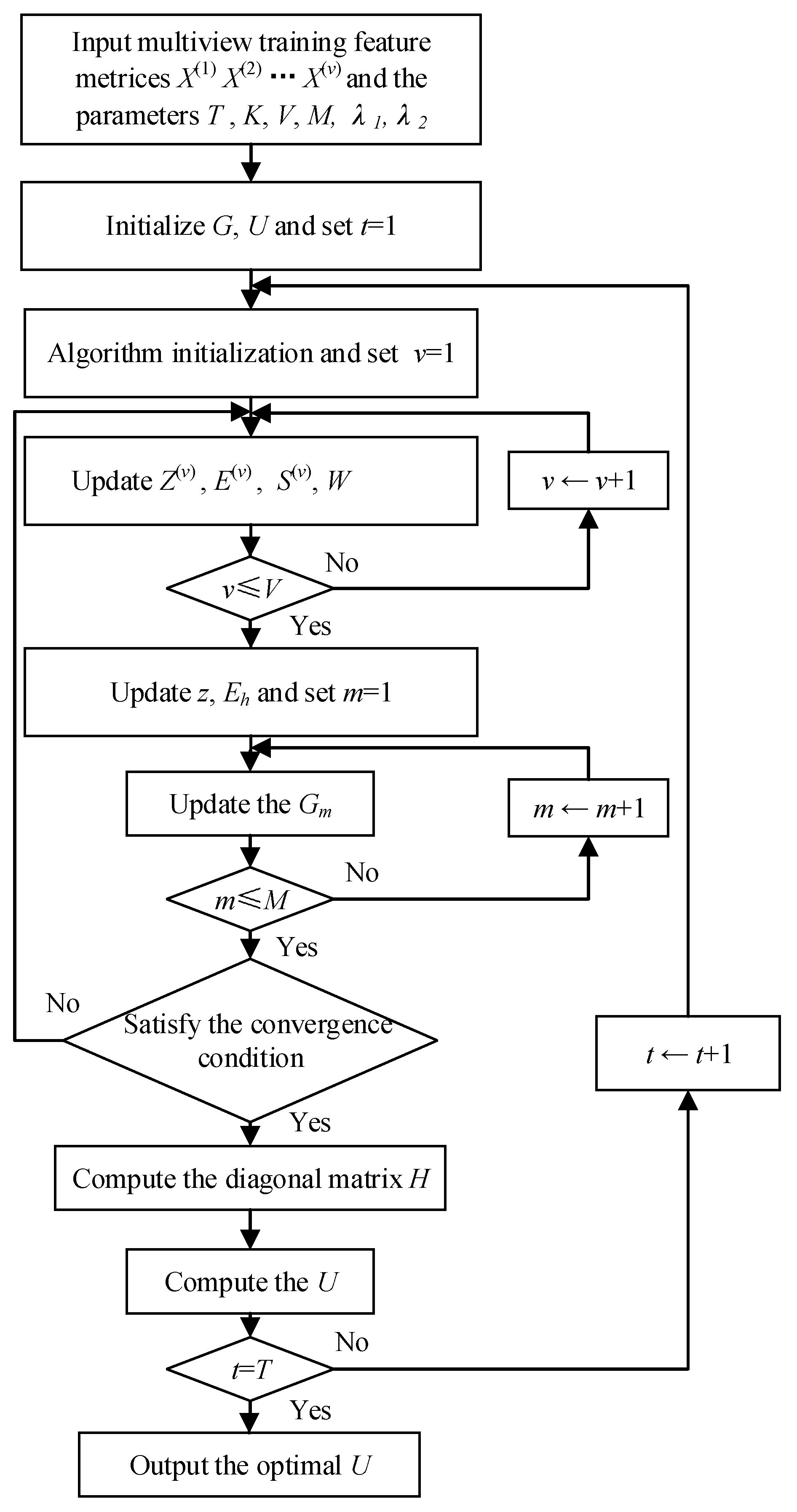
Algorithm 1 gives the steps of the optimal solution. To facilitate better understanding, the block diagram of the LR-MTR algorithm is shown in
Figure 2.
| Algorithm 1 Algorithm LR-MTR. |
| Input: Multimodal feature matrices: …, the numbers of iterations T and the cluster number K and the parameter and . |
| Output: the optimal projection U |
| initialize: Set and U as the matrix with orthogonal column vectors. |
| for … do |
| Initialize: ; ; …; |
| …; …; |
| ……; |
| …; …; |
| |
| while not comverged do |
| for each of V views do |
| Update according to Equations (10), (12), (13), (15), (16) and (18); |
| end for |
| Update z, by Equations (19) and (20); |
| for each of M modes do |
| Updata , and according to Equations (21), (22) and (23); |
| end for |
| Update by ; |
| check the convergence conditions: |
| and |
| |
| |
| ; |
| end while |
| Updata H using Equation (25). |
| Solve the eigenfunction Equation (27) to obtain the optimal U |
| end for |
| Project the samples onto the low-dimensional subspace to obtain low dimensional for classification. |
3.4. Complexity Analysis
In the optimization procedure, two-lever iteration is used to calculate the results. The first loop includes the projection matrix
U and affinity matrix
W calculations. When calculating
U, a sub-loop is also needed to iteratively update every parameter, including
,
,
,
E,
, and Lagrangian multipliers
. First, to calculate
U, the ALM optimization involves some sub-optimization problems. However, the main computation complexity
comes from multiplying the matrix in updating
,
W, and
. Second, to calculate
U, the computational complexity is from the eigen-decomposition of Equation (
27) covering
. If the LR-MTR converges in
T steps, the computational complexity is, at most,
, where
t is the loop number of the inner iteration of ALM. The outer iteration is fast (three iterations at most), so the computational burden is not too high.
3.5. Convergence Analysis
The objective function of LR-MTR is solved through alternative iterative optimization. We divide this optimization into two parts, one for updating
W and anther for
U. The suboptimization of
W is an AL-ADM process, and
U can be updated via an eigenvalue decomposition [
51,
52].
We find a function
from the objective function of Equation (
7). Then the theorem can be given.
Theorem 1. The sequence monotonically decreases in the iterative scheme.
Proof. Suppose that, in the
t-th iteration of the outer loop, we have the result from Equation (
8) as follows:
That means
updates in the inner loop have the parameters
, and
according to the AL-ADM method, which reduce the value of
in both loops, and an optimized
W is obtained. The convergence properties of the inner loop can also be proven as in the literature [
53]. Then it has
We can have
. After updating
W, we should furthermore update
U via Equation (
24). A diagonal matrix
H should be constructed in Equation (
25), and matrix
U can be obtained by a standard eigenfunction problem in Equation (
26). It has
. That will further reduce the objective value as follows:
It can be concluded from the above formulations that and , which means it is monotonically decreasing. As the equation has a positive lower bound, and due to the monotonic decrease in Theorem 1, it is simple to know that the sequence will converge to a local optimal solution. □
4. Experiments
To test the effectiveness of the LR-MTR algorithm, we run several experiments using the proposed method, which we compare with the previous algorithms. Two PolSAR data sets are used to demonstrate the LR-MTR algorithm. SVM and KNN classifiers are used for the final classification. In our experiment, terrain classification is performed by labeling each tile in a large PolSAR image with some predefined terrain category labels. In high-resolution and large-scale PolSAR image scenes, patch-level classification is more effective than pixel-level classification, as the patches contain richer terrain details which cannot be achieved by a single pixel.
4.1. Data Sets
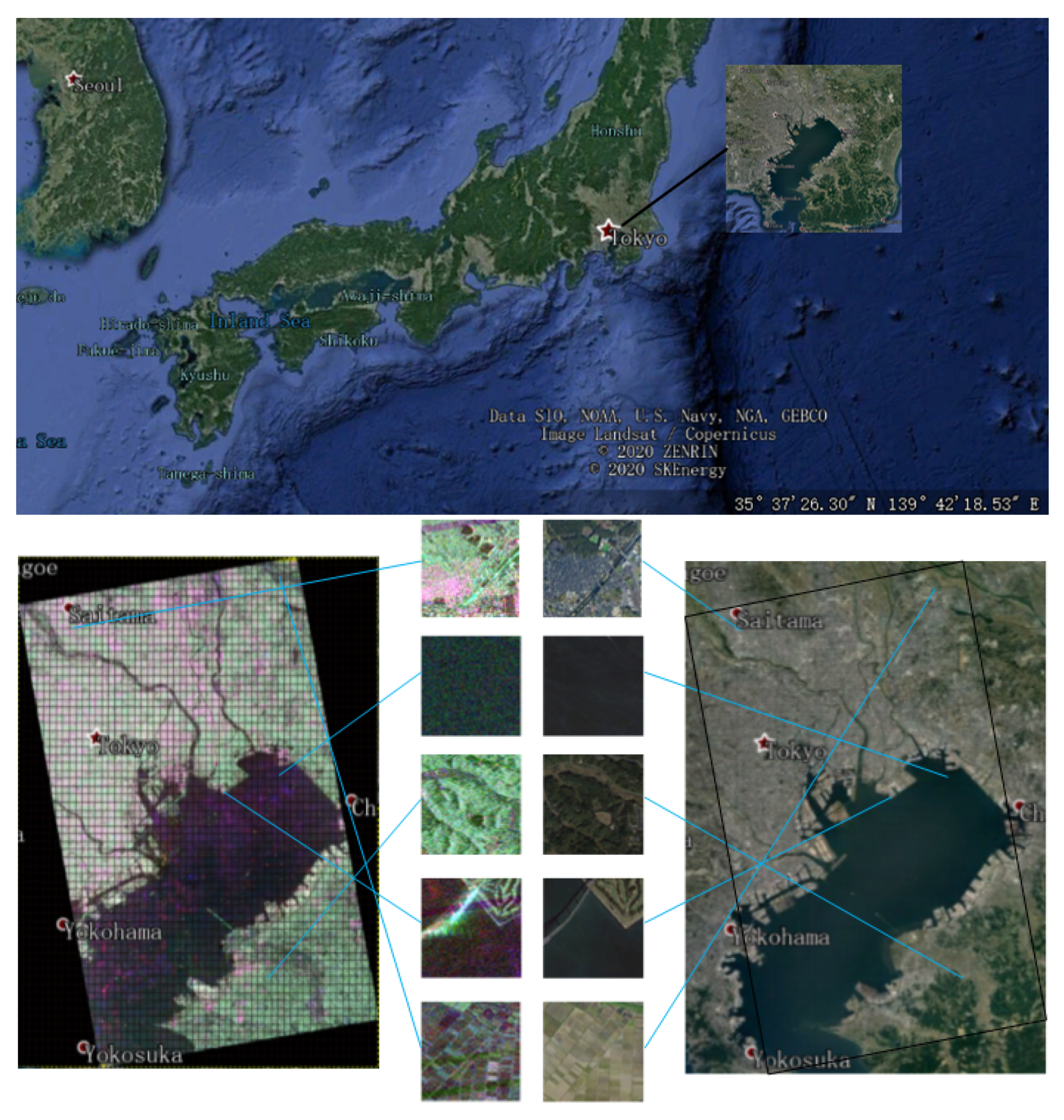
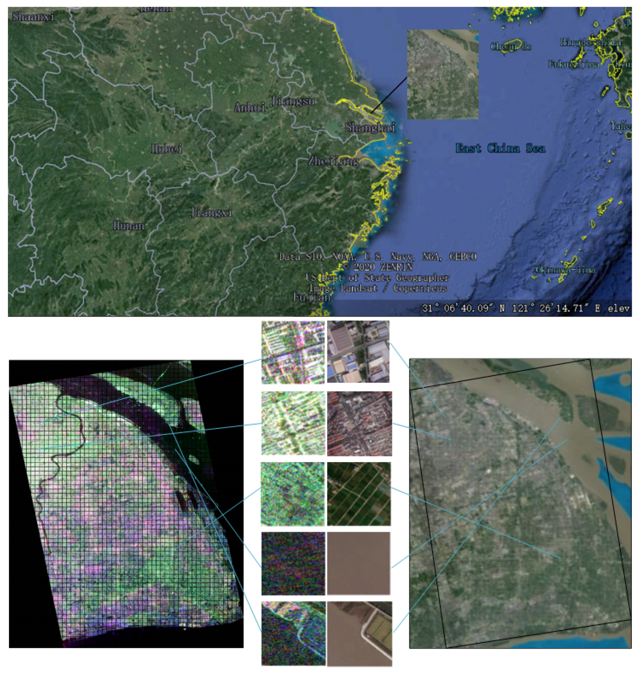
The LR-MTR method was evaluated on two data sets. One data set covers the region of Tokyo, Japan, in January 2015. The geographical location of the Tokyo data set and the scene categories are presented in
Figure 3. The Tokyo data set comes from ALOS-2 fully polarimetric SAR data, whose spatial resolution is six meters. The size of the PolSAR scene in the experiments is 14,186 × 16,514.
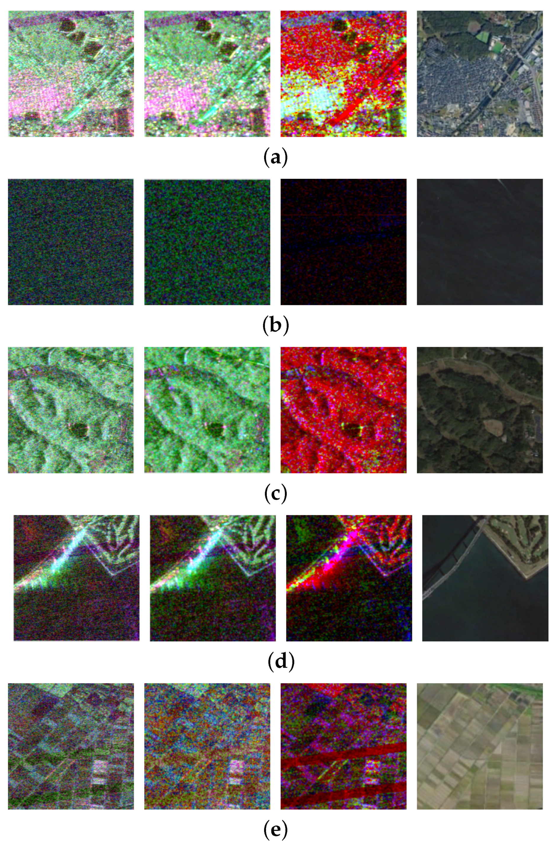
For the typical land covers, water and smooth surfaces correspond to surface scattering, rough covers to diffuse scattering, thick tree trunks and buildings to dihedral scattering, and areas of foliage to volume scattering. The patches covering all those typical land covers or jointly constructed by them are selected as the terrain categories. Then, five main terrain categories are given in the Tokyo data set: building, water, woodland, coast, and farmland. Moreover, a category which is not associated with any of the given categories is counted as the last uncertain category. The Tokyo data set is labeled with the reference of categories above. After being labeled, these data need to be preprocessed to construct the PolSAR scene data set. First, geographic calibration of the raw data is performed in the PolSARpro software. Second, Lee filtering is performed on the data. Finally, we cut the large image into small scene patches (samples). There are pixels in each sample. Then, the cut small samples are labeled. We have access to 2000 samples in the Tokyo data set. There are 855, 697, 205, 187, and 56 scenes for the building, water, woodland, coast, and farmland categories, respectively.
To extract the multimodal features, we apply the parameters from polarimetric decomposition. Further, to extract features hidden in the polarimetric phases, we use three polarimetric parameter groups: Pauli decomposition, H/alpha decomposition, and Freeman decomposition. Pauli decomposition is a typical coherency decomposition. The scattering S matrix was expressed as the complex sum of the Pauli matrices.
Figure 4 shows four images from different categories. The first column shows the Pauli image of each category, where red comes from
, green from
, and blue from
. The second column is the Cloude decomposition pseudo-color image of each category, where red represents
, green
, and blue
, as described in Figure 6.10 in [
1]. The third column is the Freeman decomposition pseudo-color image of each category, in which red is Odd, green is Dbl, and blue is Vol. The fourth column’s pictures present the category in Google Earth.
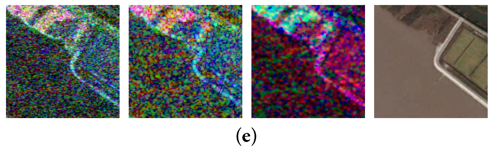
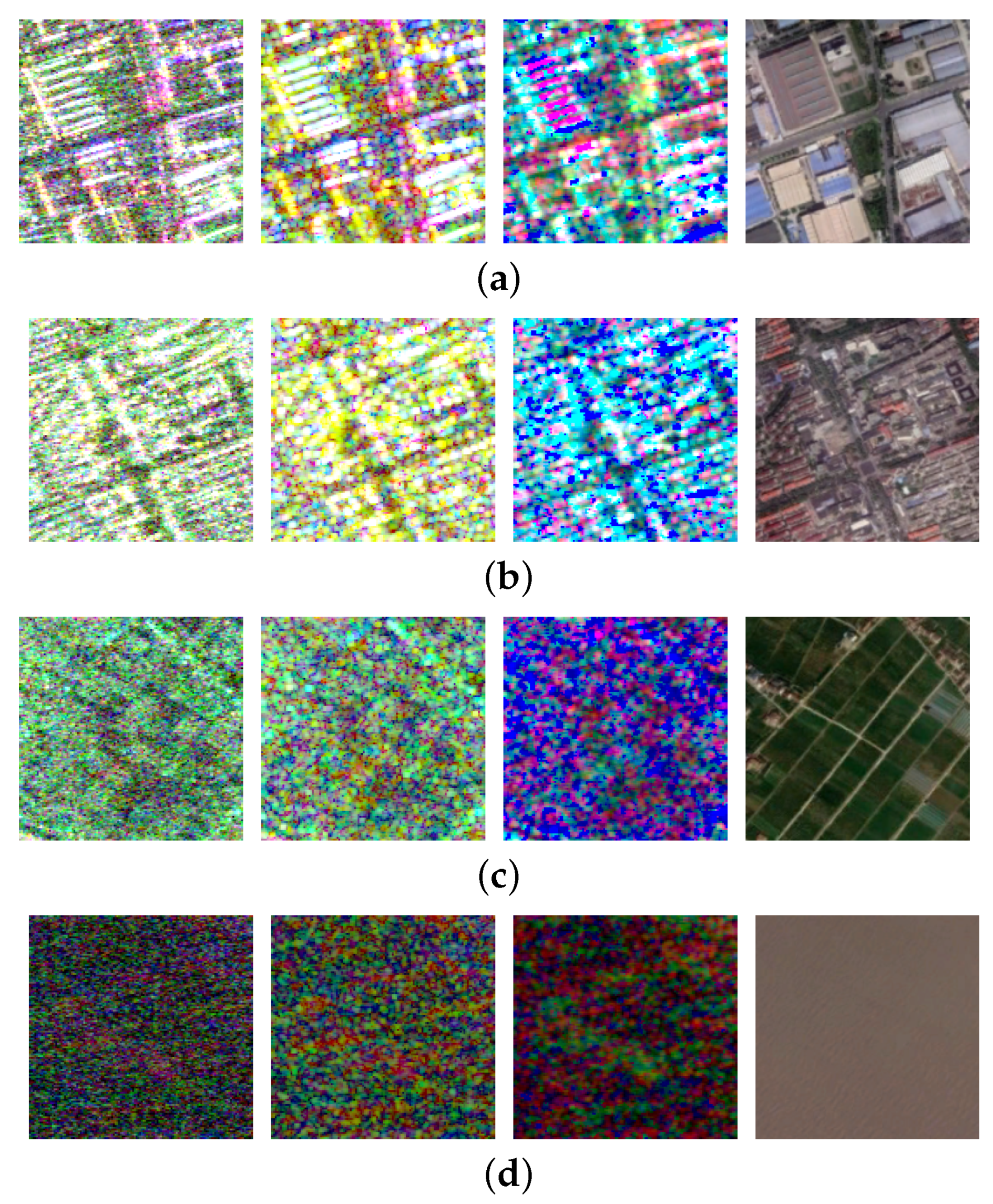
The second data set covers the region of Shanghai, China, in March 2015, as seen in
Figure 5. The geographical location of the Shanghai data set and the scene categories are presented in
Figure 3. The Shanghai data set also comes from ALOS-2. The resolution is the same as that of the Tokyo data set. The size of the labeled PolSAR scene is 8300 × 11,960, and the data set has five main categories: urban areas, suburban areas, farmland, water, and coast. Each sample has
pixels, and there are 1600 samples. There are 262, 346, 378, 417, and 197 scenes for the urban areas, suburban areas, farmland, water, and coast categories, respectively. In the Shanghai data set, we also use polarimetric decomposition to extract more multimodal features, and these four images also come from different categories in the Shanghai data set, as shown in
Figure 6, similar to the Tokyo data set.
4.2. Feature Descriptors
To evaluate the classification performance, we use two feature descriptors for comparison. Different features were extracted from the following algorithms: local binary pattern (LBP) and gray-level co-occurrence matrix (GLCM). The dimensions of GLCM and LBP are eight and fifteen, respectively. In a window, the other eight adjacent pixels are compared with the center one on the gray-scale value level, and we use the value from the center pixel as the threshold; this is where the original LBP operator comes from. If the surrounding pixels have greater values than the threshold, the position where this pixel comes from is set as 1; if not, it is set as 0. By doing so, eight pixels in the window can be calculated to generate an 8-bit binary number. The center pixel’s LBP value can be obtained, which can show the texture information of the region of interest.
4.3. Experiment Setup
To evaluate the LR-MTR algorithm, we select some different SOTA methods to compare it with in the experiments. There are linear dimension reduction algorithms (multiple dimensional scaling (MDS), independent component analysis (ICA), and principal component analysis (PCA)), linearization of manifold learning methods (such as locality preserving projection (LPP), neighbor preserving embedding (NPE), and locally linear embedding (LLE)), and nonlinear dimension reduction methods (such as kernel principal component analysis (KPCA) and stochastic neighbor embedding (SNE)). We set 15 as the number of neighbors in graph embedding algorithms. To ensure the fairness of the experiment, the features of these algorithms are reduced to a fixed dimension. Before the experiments, we need to ascertain the influence of the parameters in the experiments. The feature dimensions of the data sets also influence the algorithm performance. During data processing, training samples were selected from the whole group of samples randomly. Furthermore, in learning projection matrices, the number of training samples is important and also needs to be considered. We selected L images from each individual for the training process, and the other images in the data set were used as the test set. We set different L by the scale of each individual/object in the two data sets, i.e., L = 10, 20, 30, 40, 50, 60, and 70 for the Tokyo and Shanghai databases. In both data sets, for the LR-MTR algorithm, the M parameter was set as the same value, i.e., , and the parameter was tuned. Each task was conducted five times, and then the mean accuracy was recorded. For each comparative experiment, we tuned the parameters to their best performance. Overall accuracy (OA), average accuracy (AA), and Kappa coefficients are used to show the performance.
4.4. Experimental Result
As discussed in the last subsection, we used seven dimension reduction methods to process 24 and 45 high-dimensional features for comparison. They are composed of three modes of GLCM and LBP features. The high-dimensional features were reduced to the same dimension. The final results are recorded in two PolSAR data sets that have different typical terrain categories. The classification results and maps are shown in
Table 1,
Table 2,
Table 3 and
Table 4,
Figure 7 and
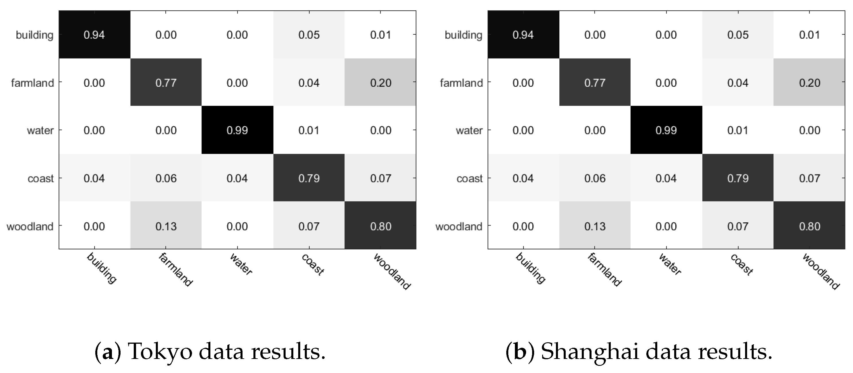
Figure 8. The confusion matrix in
Figure 7 shows that our method has good classification ability on different categories of both data sets. The classification map in
Figure 8 is randomly selected from one of the repeated experiments. Fifty samples were randomly selected to train the projection matrix
U for the linear dimension reduction algorithm, and 50 samples were used to train the classifiers (KNN and SVM). The parameter
k, which represents the nearest neighbor number, is set to 21 in the KNN classifier. The SVM classifier uses cross-validation to seek the optimal model parameters. In the following experimental analysis, a KNN classification map was used to show the visualization results.
From the classification results and classification map, it is not difficult to see that the LR-MTR algorithm has better classification performance in terms of all indices than other SOTA algorithms. For OA, the LR-MTR algorithm is approximately 2%, 2%, and 1% better than the second best algorithms. This reveals that the LR-MTR algorithm is an effective algorithm for PolSAR scene classification. In
Table 1,
Table 2,
Table 3 and
Table 4, we assign different terrain categories with the corresponding numbers. In
Table 1 and
Table 2, we use the numbers 1–5 to represent different categories: building, farmland, water, coast, and woodland, respectively. In
Table 3 and
Table 4, we use the numbers 1–5 to represent urban areas, suburban areas, water, farmland, and coast, respectively.
4.5. Experiment Analysis
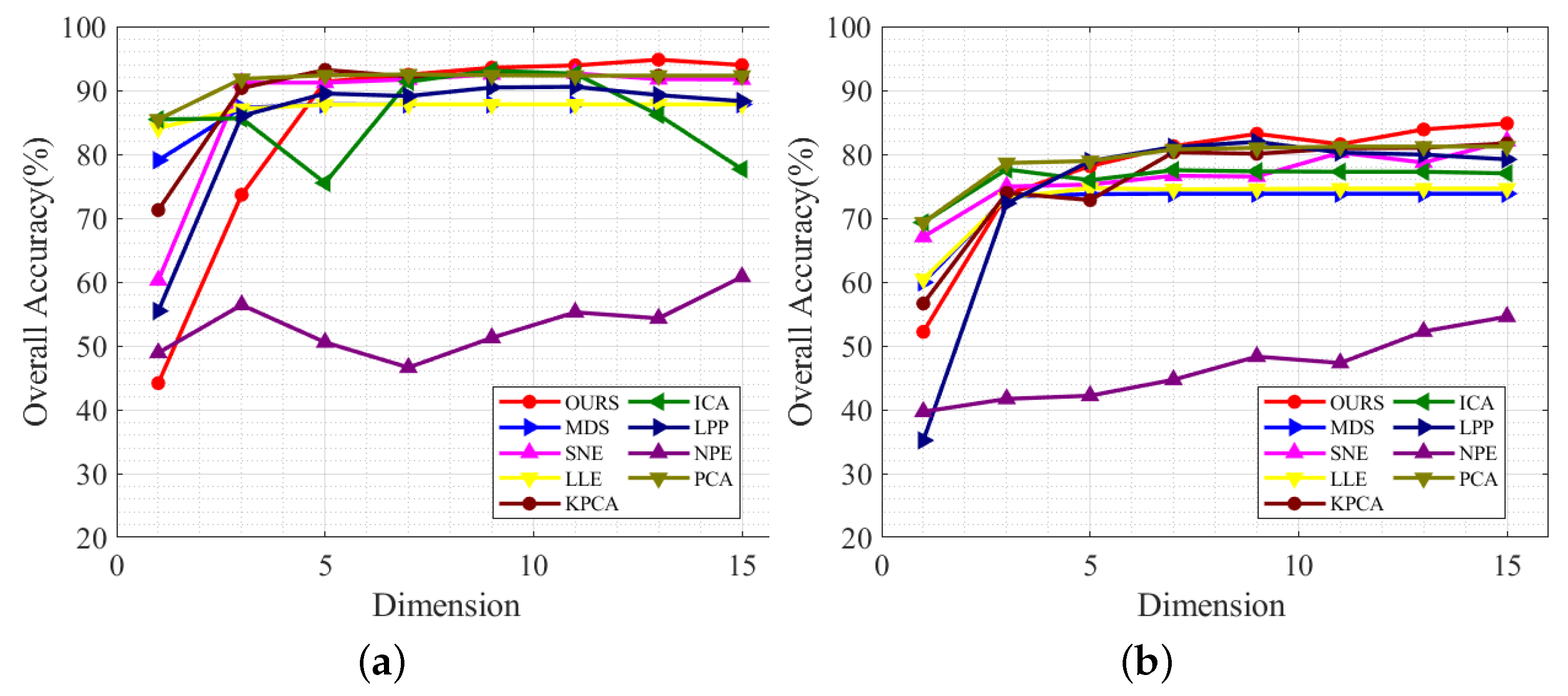
(1) Dimension: Fifty training samples were randomly selected from each category and used to learn the projection matrix
U. As the dimension changes from 1, 3, 5, …, 15, the KNN results are also affected, as shown in
Figure 8. This also shows that the LR-MTR method has a better classification accuracy than other dimension reduction algorithms when the number of dimensions is greater than seven. When it is greater than three, all algorithms except the NPE algorithm have better classification performance. Once the algorithm performance remains stable, all the algorithms will achieve better results.
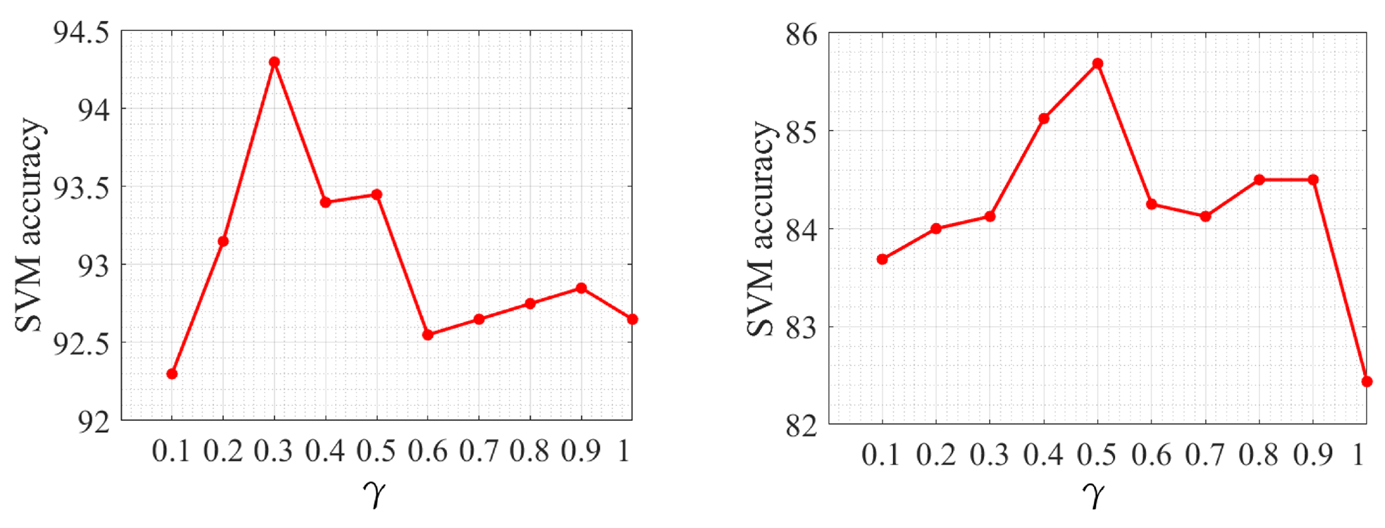
(2) Parameter Sensitivity:
Figure 9 shows the parameter tuning examples. In the LR-MTR algorithm, the balance parameter
is the most important parameter in the model. From
Figure 9, it is not difficult to find that the parameter
has some effectiveness on the two data sets. The value of
is bigger in the Shanghai data set than in the Tokyo data set for promising results. As shown in the figure, the results are different with the increase in parameters. It is not difficult to find that the parameters have certain influence on the two different data sets, and there will be an optimal parameter, but the value of the optimal parameter is different in different data sets.
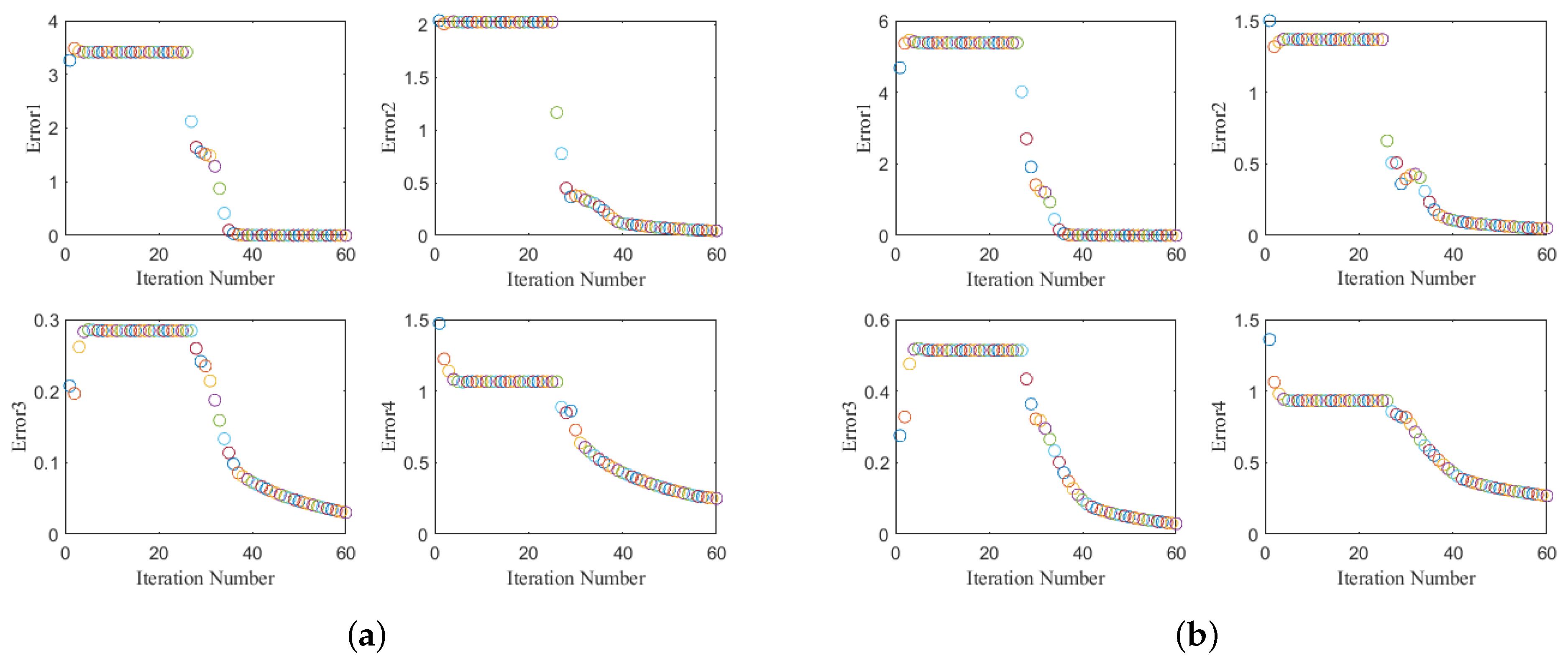
(3) Convergence: To demonstrate the convergence of the LR-MTR algorithm,
Figure 10 shows the objective values versus the iteration steps on the two representative data sets. The convergent properties of LR-MTR on the Tokyo data set and the Shanghai data set are shown in
Figure 10a,b where the errors 1–4 correspond to the computed results of the four convergence conditions in Algorithm 1, respectively. This shows that the four parameters of convergence in our method reduce as the number of iterations increases. Generally, the LR-MTR method is able to converge within 40 to 60 iterations. In the experiment, the outer loop iteration is set as two or three.
(4) Running Time: LR-MTR and the contrasting algorithms with the same number of samples (50 samples per category) were run, and the time was recorded, as shown in
Table 5. Compared with other algorithms, our algorithm cannot achieve a good performance time, as it takes more time to improve the feature representative. This is because the LR-MTR algorithm is based on an optimization algorithm with two loops, which takes more time during the convergence process. The running time can be further reduced accordingly to improve the optimal solutions.
(5) Generalization: In order to test the generalization of the proposed method, we used the learned projected matrix on another data set for classification. For a fair comparison, those DR techniques, including PCA, LPP, NPE, ICA, KPCA, LEE, SNE, and MDS, all used the same 50 samples from each category for learning the projection matrices. The OA and specific accuracy are given.
Table 6 shows the results of projection matrices learning from the Tokyo data set and being used on the Shanghai data set. Meanwhile,
Table 7 shows the results of projection matrices learning from the Shanghai data set and being used on the Tokyo data set. In the test data sets, we chose 50 samples from one data set as training samples and used the other samples for testing. From these experiments, our algorithm is able to achieve the best classification OA 79.81 (Tokyo learned U used on Shanghai data set) and 87.35 (Shanghai learned U used on Tokyo data set). This is due to the ability to capture the relevance between features, which proves that LR-MTR also has better generalization than other DR techniques.


 ,
, 


