Analysis of the Optical Turbulence Model Using Meteorological Data

Abstract

The model of atmosphere optical turbulence is important in the research field of laser atmospheric transmission, and plays a key role in astronomical site selection. In this paper, the single and overall statistical analysis between different outer scale models (HMNSP99 and the Dewan model) were conducted and the results show that the HMNSP99 model has better performance with the lowest bias, root mean square error, and center root mean square error. The results of the statistical analysis of three turbulence parameters revealed that there is a correlation between turbulence parameters and statistical operators, where statistical operators increase significantly when wind shear and temperature gradient respectively exceed 0.016 s⁻¹, 0 K/m, and the outer scale is within 2.5 m. Furthermore, a new statistical outer-scale model, the WSTG model, is proposed and the results of statistical analysis present that the WSTG model is more reliable than the HMNSP99 model in reconstructing optical turbulence strength. These results acquired from this paper add substantially to our understanding of atmosphere optical turbulence and the conclusions can be applied to improve the performance of an adaptive optics system and astronomical site selection.

1. Introduction

One of the most significant current discussions in adaptive optics (AO) systems is atmospheric optical turbulence because of its direct effects on light waves propagated in the turbulent atmosphere including scintillation, phase change, beam drift and angle-of-arrival fluctuation [1,2,3]. The primary parameter used to characterize atmospheric optical turbulence is the index of refraction structure constant $C_n^2$ [4,5,6]. In the past decades, several instruments have been developed to measure atmospheric optical turbulence, such as the meteorological balloons equipped micro-thermometer [7], SCIDAR (scintillation detection and ranging) [8], MASS (multi-aperture scintillation sensor) [9], and DIMM (differential image motion monitor) [10,11,12]. Despite their use in field testing, these instruments are expensive and difficult to operate in complicated environments, which makes estimation a less expensive and convenient alternative.

Over the years, the developments in adaptive optics have heightened the need for a $C_n^2$ estimation model. The simplest empirical model was proposed from segmented fitting on experimental data, which represent the statistically averaged results of atmospheric optical turbulence. For example, the submission laser communication (SLC) model, the Air Force Geophysics Laboratory (AFGL) and Air Force Maui Optical Station (AMOS) model, and the Critical Laser Enhancing Atmospheric Research (CLEAR I) model [13,14,15,16]. Based on the basic theory of turbulence, parameterization models were developed to establish the relationship between conventional meteorological parameters and the profiles of $C_n^2$ through the outer scale. The National Oceanic and Atmospheric Administration (NOAA) model was developed by VanZandt in 1985, which integrated the fine structure of wind shear and was relatively complex [17]. In 1988, Coulman used standard meteorological observation data to estimate $C_n^2$ profiles whose external scale was a function of altitude [18]. In 1993, based on sounding data, an outer scale model was proposed by Dewan considering the vertical shear of the horizontal wind speed [19]. Later, Trinquet established a model named AXP (with parameters A and P both functions of altitude), which indicated a vertical resolution of 300 m and a wind shear under 0.04 s⁻¹ [20]. A simple approach to estimate the $C_n^2$ profile was proposed using the Thope scale and the overturning of the temperature applied to distinguish turbulence [21]. Furthermore, Ruggiero & DeBenedictis developed an outer scale model at the Air Force Research Laboratory from the Holloman Spring 1998 and Holloman Spring 1999 thermosonde campaigns (HMNSP99), which gave the relationships relating parameterization to wind shear and temperature gradient [22]. In 2020, Bi et al. investigated the accuracy of the HMNSP99 model by comparing them with the corresponding radiosonde measurements and indicated that the estimated $C_n^2$ profiles were not completely consistent with the measured values at the corresponding altitudes [23]. The existing optical turbulence models each have their own advantages and disadvantages, and no one model is recognized as the best. Despite its drawbacks, the HMNSP99 model represents the most widely used outer scale model [23,24,25]. Due to the shortcomings of the existing optical turbulence models, improvements are needed to reflect the optical turbulence characteristics more accurately. Through a large amount of experimental data, the existing model is statistically analyzed to find the source of error, and finally a credible optical turbulence model is obtained.

This study sets out to evaluate the performance of different models, determines influencing factors of the models and develops a new model to better estimate $C_n^2$ profiles. The remainder of this paper is organized as follows: Section 2 introduces three methodologies associated with the investigation of the $C_n^2$ profiles, Section 3 provides the experimental results and discussion, including the use of contrast experiments, and, finally, Section 4 concludes the paper and proposes some limitations.

2. Experiment and Methodology

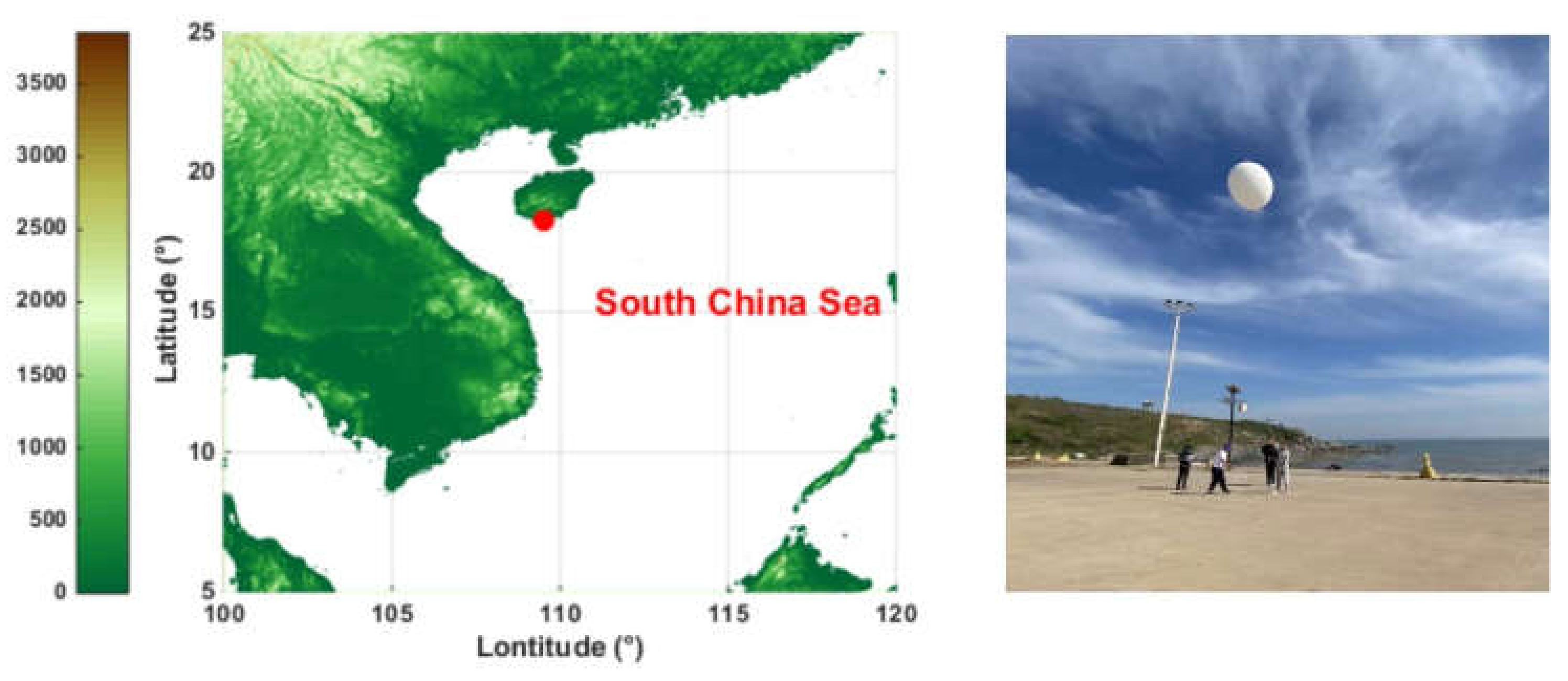
2.1. Experiment Detail

From November to December in 2017, an offshore atmospheric turbulence in situ measurement experiment was implemented in Sanya where balloon-borne radiosondes equipped with micro-thermometers and GPS was conducted by the Anhui Institute of Optics and Fine Mechanics of the Chinese Academy of Sciences. A comprehensive description of the micro-thermometer and its specifications are given in [13,14,15,16]. All the flights were released during the early morning at 7:40 a.m. or late evening at 7:40 p.m. Sanya (18.3° N, 109.5° E) is located in the South China Sea, south of Hainan Island, at an altitude of 9 m above mean sea level (AMSL), which has outstanding marine climate characteristics. The location of the experiment site and the photographs of the experimental scenario picture of the micro-thermometer are shown in Figure 1. The red point in the figure is the release position of our balloon-borne radiosondes.

2.2. Estimation Model

To obtain a vertical profile of optical turbulence strength, the parameterization models are developed to convert radiosonde meteorological parameters into the refractive index structure constant [19]. Under the assumption of local homogeneity and stationarity of the refractive index fluctuations, the parameterization model used the Tatarskii model for estimating $C_n^2$, and the profile can be expressed in the following form [4]:

$$C_n^2=a{L}_0{}^{4/3}{M}^2$$

(1)

where $a$ is a dimensionless constant set to 2.8 [26]. $L_0$ is the outer scale that mean it is the largest scale of inertial range turbulence, and the potential refractive index gradient $M$ is expressed as:

$$M=-\left(\frac{79\times {10}^{-6}P}{T}\right)\frac{\partial \ln \theta }{\partial h}$$

(2)

where $M$ is related to atmospheric temperature $\left(T\right)$, atmospheric pressure $\left(P\right)$, and potential temperature $\left(\theta \right)$. $h$ is the height above ground. $C_n^2$ can be expressed from the outer scale $L_0$ and meteorological parameters. In addition to the turbulent outer scale $L_0$, these meteorological parameters can be obtained by the balloon-borne radiosondes during the actual experiments. Therefore, it is particularly important to choose an appropriate outer scale model to estimate the $C_n^2$ profiles.

Based on the Tatarskii equation, Dewan developed an outer scale model considering the vertical shear of the horizontal wind speed, in which two expressions for the troposphere and stratosphere are proposed [19]. The outer scale model is given as follows:

$$L_0{}^{4/3}=\left\{\begin{array}{l}{0.1}^{4/3}\times {10}^{1.64+42\times S},\mathrm{T}\mathrm{r}\mathrm{o}\mathrm{p}\mathrm{o}\mathrm{s}\mathrm{p}\mathrm{h}\mathrm{e}\mathrm{r}\mathrm{e}\\ {0.1}^{4/3}\times {10}^{0.506+50\times S},\mathrm{S}\mathrm{t}\mathrm{r}\mathrm{a}\mathrm{t}\mathrm{o}\mathrm{s}\mathrm{p}\mathrm{h}\mathrm{e}\mathrm{r}\mathrm{e}\end{array}\right.$$

(3)

$$S=\sqrt{{\left(\frac{\partial u}{\partial h}\right)}^2+{\left(\frac{\partial v}{\partial h}\right)}^2}$$

(4)

where $S$ is the vertical shear of the horizontal velocity. $u$ and $v$ are two horizontal wind components. Another outer scale mode, known as the HMNSP99 model, was proposed to estimate the $C_n^2$ profiles, which takes the temperature gradient ($\frac{dT}{dh}$) and wind shear ($S$) into account [22]. For containing multiple parameters associated with the optical turbulence, the outer scale model plays an important role in estimating $C_n^2$ profiles, and its specific expression is:

$$L_0{}^{4/3}=\left\{\begin{array}{l}{0.1}^{4/3}\times {10}^{0.362+16.728S-192.347\frac{dT}{dh}},\mathrm{T}\mathrm{r}\mathrm{o}\mathrm{p}\mathrm{o}\mathrm{s}\mathrm{p}\mathrm{h}\mathrm{e}\mathrm{r}\mathrm{e}\\ {0.1}^{4/3}\times {10}^{0.757+13.819S-57.784\frac{dT}{dh}},\mathrm{S}\mathrm{t}\mathrm{r}\mathrm{a}\mathrm{t}\mathrm{o}\mathrm{s}\mathrm{p}\mathrm{h}\mathrm{e}\mathrm{r}\mathrm{e}\end{array}\right.$$

(5)

2.3. Statistical Operators

In this paper, two statistical operators of the bias and root mean square error (RMSE) operators are applied to evaluate the performance and reliability of the estimated values of different models in reconstructing optical turbulence strength [27]. The bias contains information on systematic model errors, and the RMSE contains information on the statistical errors plus the systematic errors. Furthermore, utilizing the bias and the RMSE, we retrieve the center root mean square error (CRMSE), which represents the intrinsic uncertainty not affected by the bias, and provides fundamental information on the systematic bias and statistical uncertainties. Bias refers to the difference between the estimated value and the measured value, which can be used to evaluate the accuracy of the estimated result. The smaller the absolute value of Bias, the higher the evaluation accuracy. RMSE and CRMSE reflects the degree to which the evaluated data deviates from the true value, and small RMSE and CRMSE values represent high calculation accuracy. The definition of the statistical operators is given as follows:

$$BIAS={\displaystyle \sum _{i=1}^N\frac{\left(Y_i-X_i\right)}{N}}$$

(6)

$$RMSE=\sqrt{{\displaystyle \sum _{i=1}^N\frac{{\left(Y_i-X_i\right)}^2}{N}}}$$

(7)

$$CRMSE=\sqrt{{\displaystyle \sum _{i=1}^N\frac{{\left[\left(X_i-\overline{X_i}\right)-\left(Y_i-\overline{Y_i}\right)\right]}^2}{N}}}=\sqrt{RMS{E}^2-BIA{S}^2}$$

(8)

where $X_i$ and $Y_i$ represents the estimated index values and individual measured index values from radiosonde at the same height, respectively, and $N$ is the number of samples for a couple $\left(X_i,Y_i\right)$ at the same height. $\overline{X_i}$ and $\overline{Y_i}$ stand for the average values of the measured and the model parameters, respectively. Furthermore, considering the measured value of $C_n^2$, basically in the range of10⁻¹⁹–10⁻¹⁴ m^−2/3, using log ($C_n^2$) instead of $C_n^2$ makes it easier to calculate and visualize the statistical results, which makes the results more readable. This is just a substituted conversion to represent the error of $C_n^2$ so that it is reliable and valid. When the three statistical evaluation factors are actually used, the range of reliable values has a great relationship with the magnitude of the measured data. In this paper, statistical factors (the absolute value of Bias, RMSE and CRMSE) less than 1.5 are considered to be reliable.

3. Results and Discussion

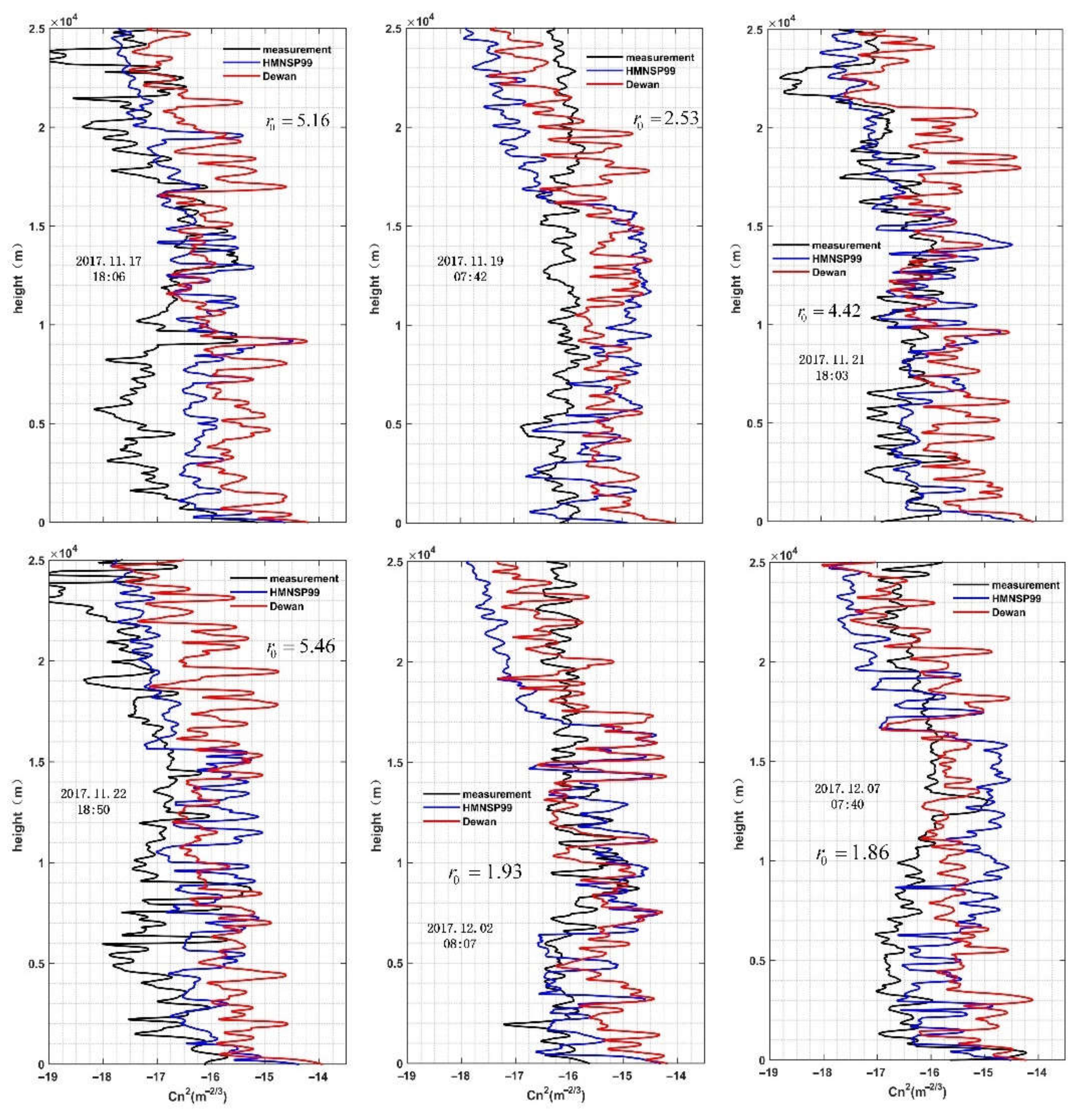
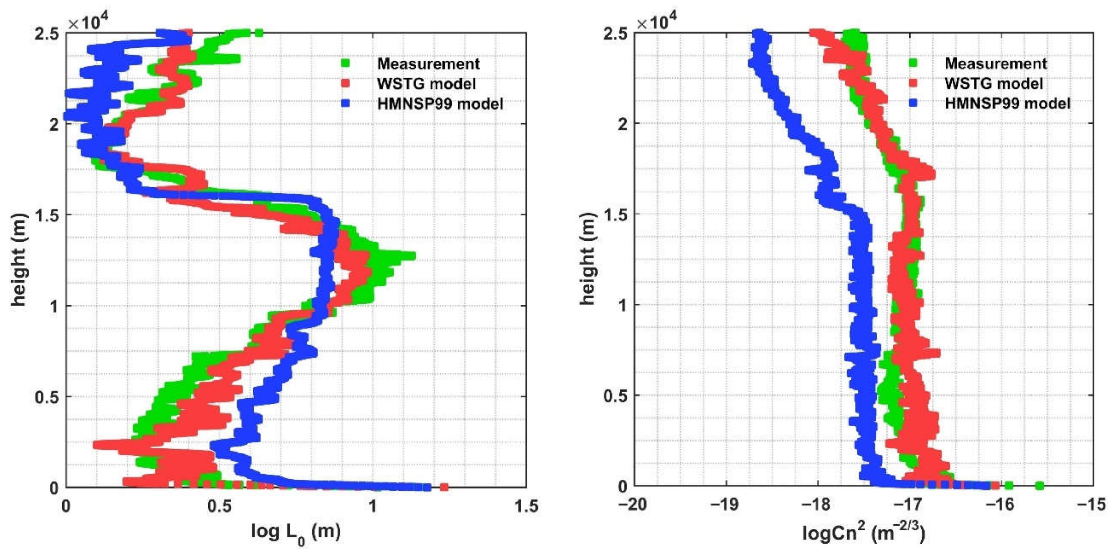
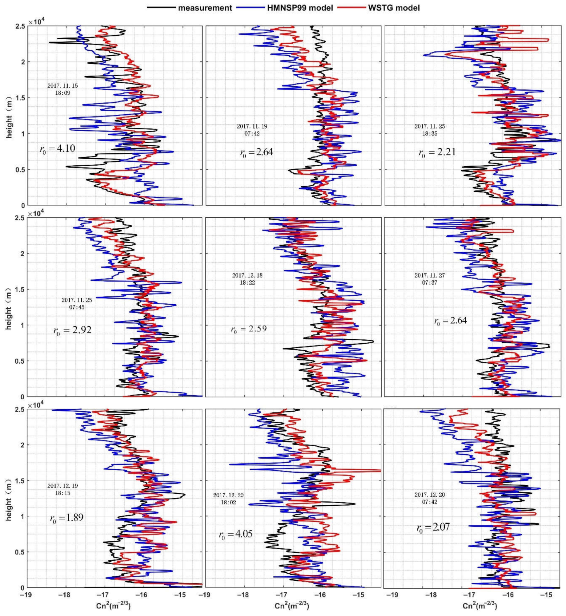
3.1. Profiles from Models and Radiosonde Measurement

In this experiment, a total of available 89 radiosonde measurements were obtained, excluding the abnormal radiosonde measurements due to various factors such as weather and strong winds. In this paper, the altitude range of the following figures is from the surface to 25 km above sea level. Figure 2 shows the $C_n^2$ profiles estimated by the models and measured by the radiosonde at the Sanya site. It is notable that the $C_n^2$ profiles reveal a steep drop around the ground. Then the $C_n^2$ values gradually increase, with altitudes from around 3 km up to 15 km and gradually decrease with altitudes in the free atmosphere thereafter. The trend between the estimated and measured profiles is consistent in general. In order to verify the turbulence strength profiles, the Fried parameters $\left(r_0\right)$ for the measured profiles are calculated in the figures. Comparing the two outer scale models, we cannot draw a definitive conclusion as to which has obvious advantages. Therefore, it is necessary to conduct a statistical analysis on the estimation results of the two outer scale models.

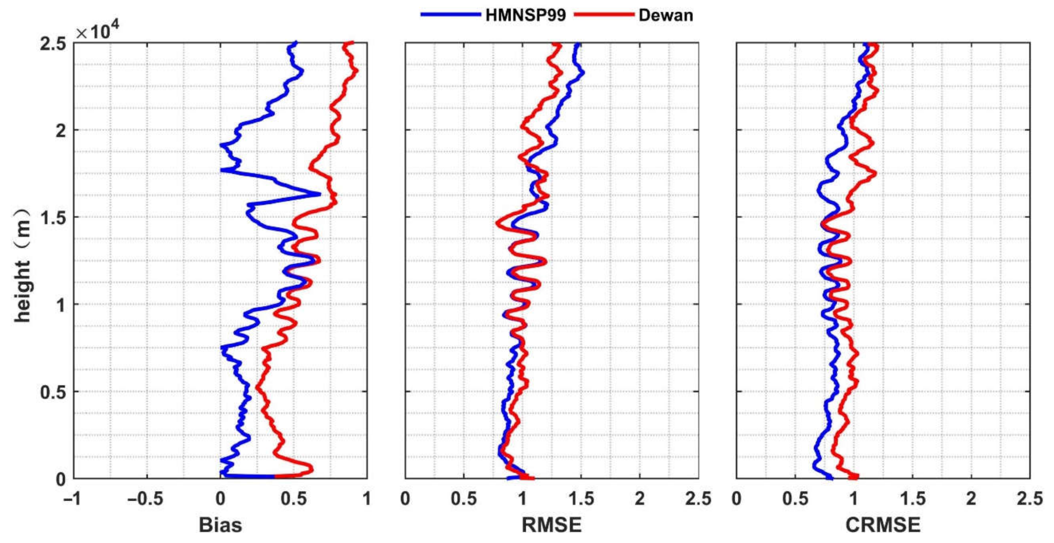
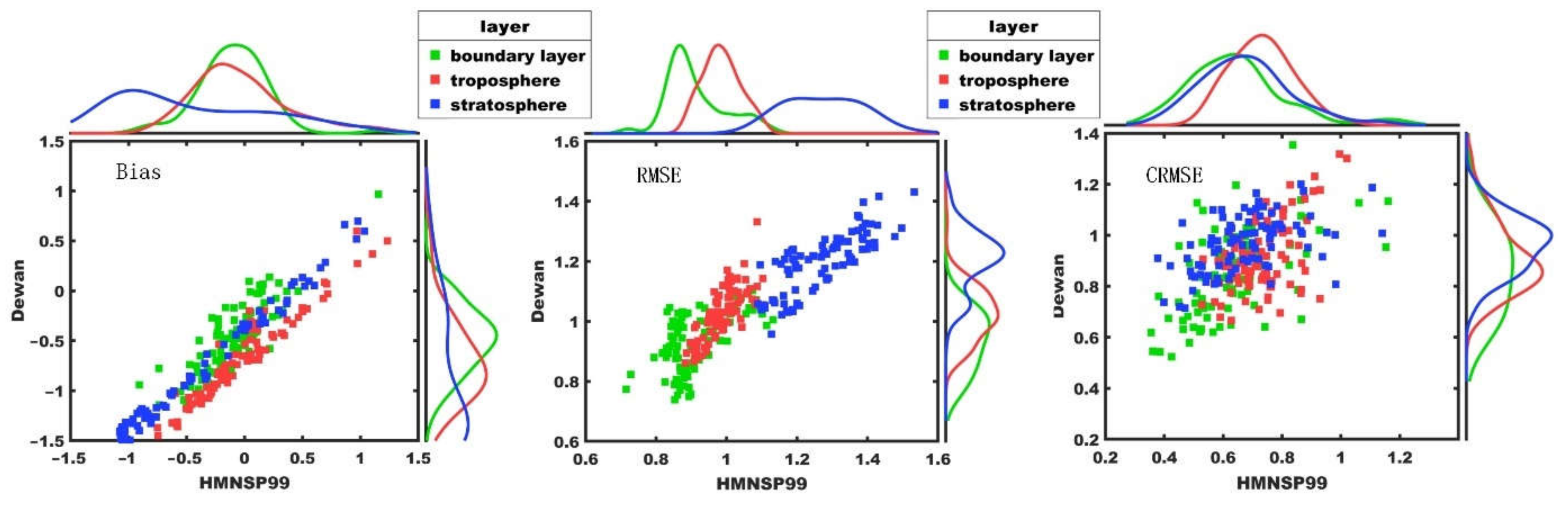
3.2. Statistical Model Performances

As can be seen from Equations (3) and (5), the outer scale models contain two expressions corresponding to the troposphere and stratosphere, respectively. Therefore, it is necessary to use statistical operators to evaluate the performance of the model hierarchically. The statistical operators for individual flights of troposphere and stratosphere between the measurements and model-based estimates are illustrated in Figure 3. According to the distribution characteristics of $C_n^2$, the statistical operator of the boundary layer is also shown here, where the statistical height is from the ground to 3 km [28]. It is notable that the bias of HMNSP99 and the Dewan models are less than 1.25 m^−2/3 and 1.75 m^−2/3, respectively. In different atmospheric stratification, the bias peaks of the two models are smaller in the boundary layer and larger in the stratosphere. It is obvious that the RMSE in the three atmospheric stratifications is significantly different, where the value gradually increases with height. The RMSE peaks of the HMNSP99 model respectively are 0.85 m^−2/3, 1 m^−2/3, and 1.3 m^−2/3 in the boundary layer, troposphere, and stratosphere. Similarly, the RMSE peaks of the Dewan model corresponds to 1 m^−2/3, 1.05 m^−2/3, and 1.25 m^−2/3. Comparing the CRMSE of different atmospheric stratifications, there is no obvious difference. However, the CRMSE of the HMNSP99 model has a range of 0.4–1.2 m^−2/3, which is smaller than the range of 0.6–1.4 m^−2/3 of the Dewan model. Overall, the estimated values of $C_n^2$ profiles using the HMNSP99 model are more consistent with the measured values than the Dewan model.

In addition, the overall statistics between the HMNSP99 and Dewan models derived from all eighty-nine balloons are performed, as shown in Figure 4, with the vertical profiles of the bias, the RMSE, and CRMSE. In this figure, $N$ is the number of flights for a couple $(X_i,Y_i)$ at each precise height and we use $N$ = 89 at each height. Moreover, the absolute value of bias is taken to better show the performance of the different models. It is obvious that bias, RMSE and CRMSE increase with altitudes. Notably, the bias of the HMNSP99 model is overall less than the Dewan model, that within 0.75 m^−2/3 and 1 m^−2/3, respectively. It is worth highlighting that the RMSE values from the Dewan model are slightly smaller than the HMNSP99 model from the ground to 15 km and larger above 15 km. Compared with the HMNSP99 model, the Dewan model has larger CRMSE values and is within 1.25 m^−2/3 from the ground up to 25 km. In conclusion, the estimated values from the HMNSP99 model are generally coherent with the radiosonde measurements. It should be pointed out that the estimated values have a relatively large drift compared with measurements above 15 km, which can obviously be seen in Figure 4.

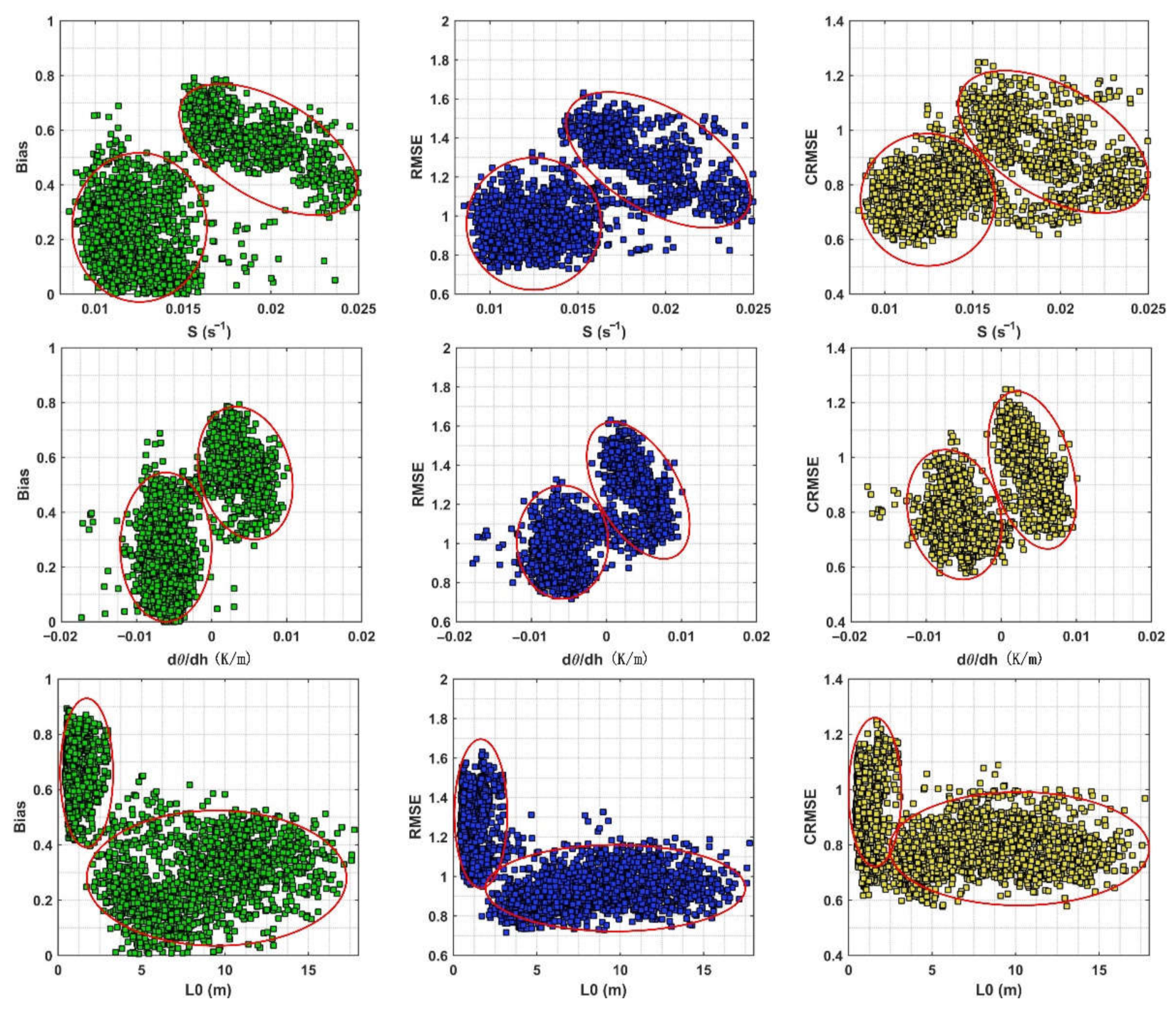
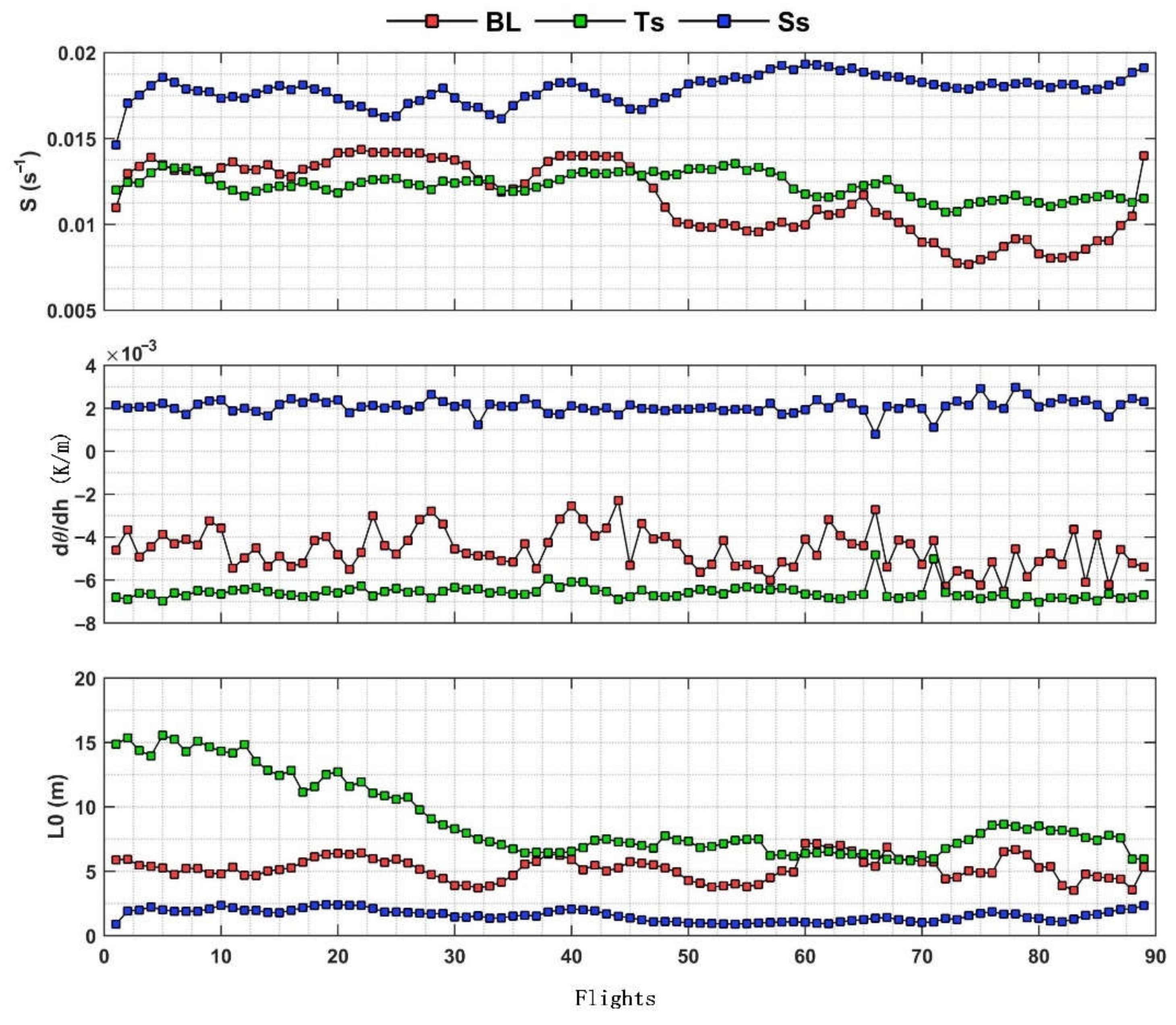
3.3. Statistical Analysis of the Effects of Turbulence Parameters

At present, despite the fact that the mechanism of the generation and development of optical turbulence is not clear, previous studies have shown that turbulence can be produced by a buoyancy heat bubble and wind shear. Therefore, temperature gradient and wind shear are widely applied to estimate optical turbulence strength [25,29,30,31,32,33]. According to Equations (3) and (5), we know that the HMNSP99 model contains more parameters relating to turbulence generation, which may lead to better model performance than the Dewan model. As mentioned previously, the HMNSP99 model was developed from the statistics of the connection between the outer scale to wind shear and temperature gradient.

In this section, we focus on the relationship between turbulence parameters (wind shear, temperature gradient and outer scale) and statistical operators (bias, RMSE and CRMSE), as described in Figure 5. It is obvious that there is a correlation between wind shear and statistical operators, where statistical operators increase significantly when wind shear exceeds 0.016 s⁻¹. This could be the result of variations in the weight of wind shear on turbulence. Therefore, when the wind shear increases, the coefficients of temperature gradient and wind shear in the model should be adjusted appropriately. Note that the statistical operators are divided into two parts by the temperature gradient, where the statistical operator increases significantly when the temperature gradient exceeds 0 km⁻¹. Generally, the temperature in the stratosphere gradually increases with height, eventually resulting in a temperature gradient of more than 0 km⁻¹. This result is consistent with the conclusions above that the stratosphere and has a larger statistical operator. Also, different outer scales also correspond to different statistical operators, where the outer scale has a critical value of 2.5 m. Differences in statistical operators may be attributed to the fact that the results of the parametric model cannot accurately reflect the fine structure of turbulence, especially small-scale turbulence.

Based on the previous statistical results, we conclude that the value of turbulence parameters will have a non-negligible impact on the performance of the model. It is necessary to perform statistical analysis on the turbulence parameters of different atmospheric layers. As shown in Figure 6, the x-axis and y-axis respectively represent the number of balloon-borne radiosondes and the average values of turbulence parameters. In addition, red, green and blue respectively represent the boundary layer, troposphere and stratosphere. It is visible that the wind shear in the stratosphere is larger than the boundary layer and troposphere, with a value exceeding 0.016 s⁻¹. Similarly, the temperature gradient increases with the boundary layer, troposphere, and stratosphere successively, and the stratosphere has the largest temperature gradient, which is close to a constant of 2 × 10⁻³ km⁻¹. In contrast, the stratosphere has the smallest outer scale, which is almost less than 2.5 m. Compared with the boundary layer and stratosphere, the outer scale of the troposphere has a larger range of 5–16 m. The differences of the outer scale can be attributed to a wider variety of turbulence strength in the stratosphere. In summary, different atmospheric layers have different turbulence parameters, which will affect the performance of the model, and finally make statistical operators present different distributions in different atmospheric layers.

3.4. New Statistical Outer Scale Model

According to previous studies, it can be demonstrated that temperature gradient and wind shear play an important role in the estimation optical turbulence strength. Compared with the Dewan model, the HMNSP99 model with the function of $S$ and $dT/dh$ can better reveal the physical mechanism of optical turbulence. However, the values of $S$ and $dT/dh$ have an important impact on the performance of the model, whose coefficients in the outer scale model become the key to accurate estimation. Therefore, using the meteorological balloons data, a new statistical outer scale model, called the WSTG model, was derived from the HMNSP99 model. In detail, first, the statistical average profiles of $L_0$, $S$, and $dT/dh$ with a vertical resolution of 100 m are acquired from the meteorological balloons data. Second, according to the value of $S$ and $dT/dh$, $L_0$, $S$ and $dT/dh$ are used for piecewise fitting to develop the WSTG model. Finally, a new outer scale model is obtained through constant fitting, where the residual sum of squares between measured values and estimations are minimized. Its specific expression is:

$$L_0{}^{4/3}=\left\{\begin{array}{l}{0.1}^{4/3}\times {10}^{0.835-37.164S-306.034\frac{dT}{dh}},S<0.016\cap dT/dh<0\\ {0.1}^{4/3}\times {10}^{0.825+66.9S-52.783\frac{dT}{dh}},S<0.016\cap dT/dh>0\\ {0.1}^{4/3}\times {10}^{0.715+52.907S-102.515\frac{dT}{dh}},S>0.016\cap dT/dh<0\\ {0.1}^{4/3}\times {10}^{2.215-9.882S-101.666\frac{dT}{dh}},S>0.016\cap dT/dh>0\end{array}\right.$$

(9)

In this part, attention has been given to evaluate the performance of the newly proposed WSTG model. Figure 7 presents statistically average profiles of $L_0$ and $C_n^2$ between the estimations calculated by models and the radiosonde measurements. It is notable that the $L_0$ and $C_n^2$ profiles of estimated and measured are consistent in the trend in general. Comparing the $L_0$ profiles of two estimation models, the differences between the WSTG model and measurement are relatively minor from ground up to 25 km. It should be pointed out that the $C_n^2$ profiles between WSTG model and measurements present better agreement as a whole, but the $C_n^2$ values from the HMNSP99 model have a relatively large drift compared with measurements above 15 km, which can be clearly seen in Figure 7. Overall, the WSTG model performs better than the HMNSP99 model in reconstructing the optical turbulence strength.

In order to ensure the applicability of the newly proposed WSTG model, the comparisons of the estimated $C_n^2$ profiles obtained by the two outer scale models (HMNSP99 and WSTG) for individual meteorological balloons in Sanya, along with the measured $C_n^2$ profiles, are depicted in Figure 8. It is clear that the HMNSP99 and WSTG model are in alignment with the measured values in trends as a whole, but the WSTG model has better estimation results in magnitude. The differences between two models are relatively small from ground up to 15 km, and more obvious above 15 km. However, there is still some room to improve the WSTG model, especially above 20 km. In other words, despite the fact that the WSTG model is not perfect, its performance has been greatly improved compared to the HMNSP99 model.

In addition, the statistical operators between the estimations calculated by models (HMNSP99 and WSTG) and the radiosonde measurements from all eighty-nine flights are performed, as shown in Figure 9. It is obvious that the absolute values of the bias of the WSTG model are less than or equal to the HMNSP99 model for most of the flights, which have a range of −0.5–0.5. Similarly, the RMSE of the WSTG model are smaller than the HMNSP99 model for most of flights as well as less than 0.8 and 1.2, respectively. Despite the fact that the differences in CRMSE between the two models are relatively minor, the CRMSE of the WSTG model are still smaller than the HMNSP99 model as a whole. In conclusion, in consideration of the individual statistical analyses, the WSTG model is more reliable than the HMNSP99 model in reconstructing optical turbulence strength.

4. Conclusions

In this investigation, the balloon-borne radiosondes equipped with micro-thermometers are released to require the $C_n^2$ profiles and conventional meteorological parameters at Sanya, south of the Hainan Island. Returning to the purpose posed at the beginning of the study, this study set out to evaluate the performance of different models, determine influencing factors of the models and developed a new model to better estimate $C_n^2$ profiles. In order to achieve satisfactory results for this goal, this research first statistically analyzed the performance of different outer-scale models (HMNSP99 and Dewan model) in different atmospheric layers using three statistical operators (bias, RMSE and CRMSE). After that, we put our attention to the influence of turbulence parameters on statistical operators and the turbulence parameters of different atmospheres. Finally, a new model containing wind shear and temperature gradient used to estimate $C_n^2$ profiles was proposed from the results of statistical analysis. The conclusions are summarized as follows.

According to the individual and overall statistical analysis results, the HMNSP99 model has better performance with the lowest bias, RMSE, and CRMSE than the Dewan model, which includes the results of different atmosphere layers. On the one hand, the individual statistical analysis results indicate that the bias of the HMNSP99 model are less than 1.25 m^−2/3 and the RMSE peaks respectively are 0.85 m^−2/3, 1 m^−2/3 and 1.3 m^−2/3 in the boundary layer, troposphere, and stratosphere. Also, the CRMSE of the HMNSP99 model has a range of 0.4–1.2 m^−2/3, which is smaller than the range of 0.6–1.4 m^−2/3 of the Dewan model. On the other hand, the overall statistical analysis results show that that bias, RMSE and CRMSE increase with altitudes. The bias and RMSE of the HMNSP99 model respectively are within 0.75 m^−2/3 and 1.5 m^−2/3 from the ground up to 25 km. In a word, the estimated values of $C_n^2$ profiles using the HMNSP99 model are more consistent with the measured values, but the estimated values have a relatively large drift in the stratosphere (above 15 km).

Three turbulence parameters analysis revealed that there is a correlation between turbulence parameters and statistical operators, where statistical operators increase significantly when wind shear and temperature gradient exceed 0.016 s⁻¹ and 0 km⁻¹, respectively. Similarly, the outer scale has a critical value, where statistical operators increase significantly when the outer scale is within 2.5 m. Moreover, this paper has performed statistical analysis on the turbulence parameters of different atmospheric layers. It has shown that the wind shear and temperature gradient in the stratosphere is larger than the boundary layer and troposphere, which respectively exceed 0.016 s⁻¹ and 0 km⁻¹. In contrast, the stratosphere has the smallest outer scale, which is almost less than 2.5 m.

A new statistical outer-scale model, the WSTG model, is proposed based on the results of previous statistical analyses. To evaluate the performance of the newly proposed model, the comparisons of the estimated $C_n^2$ profiles from the HMNSP99 and WSTG models for individual meteorological balloons is carried out. It is apparent that the HMNSP99 and WSTG models are in good agreement with the measured values in trends as a whole, but the WSTG model has better estimation results in magnitude. Furthermore, the HMNSP99 and WSTG models are applied to calculate statistical operators of individual meteorological balloons and the results suggest that the WSTG model is more reliable than the HMNSP99 model in reconstructing optical turbulence strength.

This work was undertaken to evaluate the performance of the most used optical turbulence models and to propose a new outer scale model through statistical analysis. These results add substantially to our understanding of atmosphere optical turbulence and the conclusions may be applied to improve the performance of an adaptive optics system and astronomical site selection. The newly proposed optical turbulence model can be used to estimate optical turbulence strength, especially in harsh and complex environments, where it is impractical and expensive to deploy instrumentation to characterize the atmospheric turbulence. However, these results are limited by the time and position of the experiment. It is recommended that future analysis should include more comprehensive data and the performance of the WSTG model needs further verification in different regions, seasons, and weather conditions.

References

1. Ata, Y.; Baykal, Y.; Gökçe, M.C. Average channel capacity in anisotropic atmospheric non-Kolmogorov turbulent medium. Opt. Commun. 2019, 451, 129–135. [Google Scholar] [CrossRef]
2. Baykal, Y.; Gerçekcioğlu, H. Multimode laser beam scintillations in strong atmospheric turbulence. Appl. Phys. B 2019, 125, 152. [Google Scholar] [CrossRef]
3. Mahalov, A.; McDaniel, A. Long-range propagation through inhomogeneous turbulent atmosphere: Analysis beyond phase screens. Phys. Scr. 2019, 94, 034003. [Google Scholar] [CrossRef]
4. Tatarski, V.I.; Silverman, R.A.; Chako, N. Wave Propagation in a Turbulent Medium. Phys. Today 1961, 14, 46. [Google Scholar] [CrossRef]
5. Hutt, D.L. Modeling and measurement of atmospheric optical turbulence over land. Opt. Eng. 1999, 38, 1288. [Google Scholar] [CrossRef]
6. Roddier, F. V The Effects of Atmospheric Turbulence in Optical Astronomy. In Progress in Optics; Wolf, E., Ed.; Elsevier: Amsterdam, The Netherlands, 1981; Volume 19, pp. 281–376. [Google Scholar]
7. Azouit, M.; Vernin, J. Optical Turbulence Profiling with Balloons Relevant to Astronomy and Atmospheric Physics. Publ. Astron. Soc. Pac. 2005, 117, 536–543. [Google Scholar] [CrossRef]
8. Avila, R.; Vernin, J.; Masciadri, E. Whole atmospheric-turbulence profiling with generalized scidar. Appl. Opt. 1997, 36, 7898–7905. [Google Scholar] [CrossRef]
9. Kornilov, V.; Tokovinin, A.; Shatsky, N.; Voziakova, O.; Potanin, S.; Safonov, B. Combined MASS-DIMM instrument for atmospheric turbulence studies. Mon. Not. R. Astron. Soc. 2007, 382, 1268–1278. [Google Scholar] [CrossRef] [Green Version]
10. McHugh, J.; Jumper, G.; Chun, M. Balloon Thermosonde Measurements over Mauna Kea and Comparison with Seeing Measurements. Publ. Astron. Soc. Pac. 2008, 120, 1318–1324. [Google Scholar] [CrossRef]
11. Wang, Z.; Zhang, L.; Kong, L.; Bao, H.; Guo, Y.; Rao, X.; Zhong, L.; Zhu, L.; Rao, C. A modified S-DIMM+: Applying additional height grids for characterizing daytime seeing profiles. Mon. Not. R. Astron. Soc. 2018, 478, 1459–1467. [Google Scholar] [CrossRef]
12. Scharmer, G.B.; van Werkhoven, T.I.M.J.A. S-DIMM+ height characterization of day-time seeing using solar granulation. Astron. Astrophys. 2010, 513, A25. [Google Scholar] [CrossRef]
13. Miller, M.; Zieske, P. Turbulence Environment Characterization; Interim Report; Avco-Everett Research Lab: Wilmington, MA, USA, 1979; p. 135. [Google Scholar]
14. Good, R.E.; Beland, R.R.; Murphy, E.A.; Brown, J.H.; Dewan, E.M. Atmospheric models of optical turbulence. Proc. SPIE 1988, 928, 165–186. [Google Scholar] [CrossRef]
15. Jumper, G.; Beland, R. Progress in the understanding and modeling of atmospheric optical turbulence. In Proceedings of the 31st Plasmadynamics and Lasers Conference, Denver, CO, USA, 19–22 June 2000. [Google Scholar]
16. Beland, R.R.; Brown, J.H. A deterministic temperature model for stratospheric optical turbulence. Phys. Scr. 1988, 37, 419–423. [Google Scholar] [CrossRef]
17. Warnock, J.M.; Vanzandt, T.E. A statistical model to estimate refractivity turbulence structure constant Cn2 in the free atmosphere. Int. Counc. Sci. Unions Middle Atmos. Program. Handb. MAP 1986, 20, 166. [Google Scholar]
18. Coulman, C.E.; Vernin, J.; Coqueugniot, Y.; Caccia, J.L. Outer Scale of Turbulence Appropriate to Modeling Refractive-Index Structure Profiles. Appl. Opt. 1988, 27, 155–160. [Google Scholar] [CrossRef]
19. Dewan, E.; Good, R.; Beland, R.; Brown, J. A Model for Cn(2) (Optical Turbulence) Profiles Using Radiosonde Data; Phillips Laboratory, Directorate of Geophysics, Air Force Materiel Command: Hanscom AFB, MA, USA, 1993; p. 50. [Google Scholar]
20. Trinquet, H.; Vernin, J. A Model to Forecast Seeing and Estimate C2N Profiles from Meteorological Data. Publ. Astron. Soc. Pac. 2006, 118, 756–764. [Google Scholar] [CrossRef] [Green Version]
21. Basu, S. A simple approach for estimating the refractive index structure parameter (Cn2) profile in the atmosphere. Opt. Lett. 2015, 40, 4130–4133. [Google Scholar] [CrossRef]
22. Ruggiero, F.H.; Debenedictis, F.H. Forecasting optical turbulence from mesoscale numerical weather prediction models. In Proceedings of the In Proceedings of the DoD High Performance Modernization Program Users Group Conference, Austin, TX, USA, 10–14 June 2002. [Google Scholar]
23. Bi, C.; Qian, X.; Liu, Q.; Zhu, W.; Li, X.; Luo, T.; Wu, X.; Qing, C. Estimating and measurement of atmospheric optical turbulence accordingto balloon-borne radiosonde for three sites in China. J. Opt. Soc. Am. A 2020, 37, 1785–1794. [Google Scholar] [CrossRef]
24. Qing, C.; Wu, X.; Li, X.; Luo, T.; Su, C.; Zhu, W. Mesoscale optical turbulence simulations above Tibetan Plateau: First attempt. Opt. Express 2020, 28, 4571–4586. [Google Scholar] [CrossRef]
25. Han, Y.; Wu, X.; Luo, T.; Qing, C.; Yang, Q.; Jin, X.; Liu, N.; Wu, S.; Su, C. New Cn2 statistical model based on first radiosonde turbulence observation over Lhasa. J. Opt. Soc. Am. A 2020, 37, 995–1001. [Google Scholar] [CrossRef] [PubMed]
26. Abahamid, A.; Jabiri, A.; Vernin, J.; Zouhair, B.; Azouit, M.; Agabi, A. Optical turbulence modeling in the boundary layer and free atmosphere using instrumented meteorological balloons. Astron. Astrophys. 2004, 416, 1193–1200. [Google Scholar] [CrossRef] [Green Version]
27. Masciadri, E.; Lascaux, F.; Fini, L. MOSE: Operational forecast of the optical turbulence and atmospheric parameters at European Southern Observatory ground-based sites—I. Overview and vertical stratification of atmospheric parameters at 0–20 km. Mon. Not. R. Astron. Soc. 2013, 436, 1968–1985. [Google Scholar] [CrossRef] [Green Version]
28. Kovadlo, P.G.; Shikhovtsev, A.Y.; Kopylov, E.A.; Kiselev, A.V.; Russkikh, I.V. Study of the Optical Atmospheric Distortions using Wavefront Sensor Data. Russ. Phys. J. 2021, 63, 1952–1958. [Google Scholar] [CrossRef]
29. Wu, S.; Su, C.; Wu, X.; Luo, T.; Li, X. A Simple Method to Estimate the Refractive Index Structure Parameter (${C}_{n}^{2}$) in the Atmosphere. Publ. Astron. Soc. Pac. 2020, 132, 084501. [Google Scholar] [CrossRef]
30. Wu, S.; Wu, X.; Su, C.; Yang, Q.; Xu, J.; Luo, T.; Huang, C.; Qing, C. Reliable model to estimate the profile of the refractive index structure parameter (Cn2) and integrated astroclimatic parameters in the atmosphere. Opt. Express 2021, 29, 12454–12470. [Google Scholar] [CrossRef]
31. Wu, S.; Hu, X.; Han, Y.; Wu, X.; Su, C.; Luo, T.; Li, X. Measurement and analysis of atmospheric optical turbulence in Lhasa based on thermosonde. J. Atmos. Sol. Terr. Phys. 2020, 201, 105241. [Google Scholar] [CrossRef]
32. Shao, S.; Qin, F.; Xu, M.; Liu, Q.; Han, Y.; Xu, Z. Temporal and spatial variation of refractive index structure coefficient over South China sea. Results Eng. 2020, 9, 100191. [Google Scholar] [CrossRef]
33. Han, Y.; Yang, Q.; Nana, L.; Zhang, K.; Qing, C.; Li, X.; Wu, X.; Luo, T. Analysis of wind-speed profiles and optical turbulence above Gaomeigu and the Tibetan Plateau using ERA5 data. Mon. Not. R. Astron. Soc. 2021, 501, 4692–4702. [Google Scholar] [CrossRef]
Figure 1. Location of experiment site (left) and experimental scenario picture of balloon-borne micro-thermometer (right).
Remotesensing 14 03085 g001
Figure 2. Comparison of C n 2 profiles between measurements by radiosonde and estimations by HMNSP99 and Dewan model.
Remotesensing 14 03085 g002
Figure 3. Statistical analysis of log C n 2 calculated by HMNSP99 and Dewan model for eighty-nine flights of individual meteorological balloons.
Remotesensing 14 03085 g003
Figure 4. Overall statistical analysis of log C n 2 profiles of eighty-nine balloon flights.
Remotesensing 14 03085 g004
Figure 5. Statistical analysis of the relationship between statistical operators and turbulence parameters.
Remotesensing 14 03085 g005
Figure 6. Statistically average turbulence parameters in different atmospheric layers. BL: boundary layer; Ts: troposphere; Ss: stratosphere.
Remotesensing 14 03085 g006
Figure 7. Statistically average profiles of L 0 and C n 2 from models and radiosonde measurement.
Remotesensing 14 03085 g007
Figure 8. Comparison between estimated C n 2 profiles using the HMNSP99 model (blue), the WSTG model (red), and the measured profiles (black).
Remotesensing 14 03085 g008
Figure 9. Statistical analysis of log C n 2 calculated by HMNSP99 and WSTG model for eighty-nine flights of individual meteorological balloons.
Remotesensing 14 03085 g009
Publisher’s Note: MDPI stays neutral with regard to jurisdictional claims in published maps and institutional affiliations.