Article

A New Automatic Extraction Method for Glaciers on the Tibetan Plateau under Clouds, Shadows and Snow Cover

1
School of Earth Science and Technology, Zhengzhou University, Zhengzhou 450001, China
2
Joint Laboratory of Eco-Meteorology, Chinese Academy of Meteorological Sciences, Zhengzhou University, Zhengzhou 450001, China
3
State Key Laboratory of Severe Weather, Chinese Academy of Meteorological Sciences, Beijing 100081, China
4
Collaborative Innovation Center on Forecast Meteorological Disaster Warning and Assessment, Nanjing University of Information Science & Technology, Nanjing 210044, China
*
Author to whom correspondence should be addressed.
Remote Sens. 2022, 14(13), 3084; https://doi.org/10.3390/rs14133084
Submission received: 2 June 2022 / Revised: 23 June 2022 / Accepted: 24 June 2022 / Published: 27 June 2022

Abstract

:
Accurately assessing the dynamic changes of glaciers under the background of climate warming is of great significance for taking scientific countermeasures to cope with climate change. Aiming at the difficulties of glacier identification, such as mountain and cloud shadow, cloud cover and seasonal snow cover in high altitude areas, this paper proposes a reflectivity difference index for identifying glaciers in shadow and glacial lakes and a multi-temporal minimum band ratio index for reducing the influence of snow cover. It establishes a new large-scale glacier extraction method (so-called Double RF) based on the random forest algorithm of Google Earth Engine (GEE) and applies it to the Tibetan Plateau. The verification results based on 30% sample points show that overall accuracies of the first and second classification of 96.04% and 90.75%, respectively, and Kappa coefficients of 0.92 and 0.83, respectively. Compared with the real glacier dataset, the percentage of correctly extracted glacier area of the total area of glacier dataset (PGD) was 84.07%, and the percentage of correctly extracted glacier area of the total area of extracted glacier (PGE) was 89.06%; the harmonic mean (HM) of the two was 86.49%. The extraction results were superior to the commonly used glacier extraction methods: the band ratio method based on median composite image (Median_Band) (HM = 79.47%), the band ratio method based on minimum composite image (Min_Band) (HM = 81.19%), the normalized difference snow cover index method based on median composite image (Median_NDSI) (HM = 83.48%), the normalized difference snow cover index method based on minimum composite image (Min_NDSI) (HM = 84.08%), the random forest method based on median composite image (Median_RF) (HM = 83.87%) and the random forest method based on minimum composite image (Min_RF) (HM = 85.36%). The new glacier extraction method constructed in this study could significantly improve the identification accuracy of glaciers under the influences of shadow, snow cover, cloud cover and debris. This study provides technical support for obtaining long-term glacier distribution data on the Tibetan Plateau and revealing the impact of climate warming on glaciers on the Tibetan Plateau.

1. Introduction

Glaciers are formed by ice-accumulating processes, such as compaction, recrystallization, and refreezing of a large amount of snow throughout the year [1]. They are important components of the cryosphere and one of the best natural indicators of climate change [2] and are mainly distributed in high altitude and high latitude areas. The Tibetan Plateau is known as the “roof of the world” and the “Asian Water Tower”; glacier changes in the region will have a significant impact on the regional and even the global climate, water cycles, sea level changes, and regional ecological evolution and socio-economic development [3,4]. Understanding the temporal and spatial changes of glaciers on the Tibetan Plateau is of great significance for accurately assessing the impact of climate change on glaciers and scientifically formulating countermeasures to help cope with climate change.
The boundary of glaciers is an important feature to accurately evaluate glacier distribution and area variation [5]. At present, methods for automatic or semi-automatic glacier mapping based on remote sensing information include normalized difference snow index (NDSI) [6,7], the band ratio method [8], supervised classification of random forest (RF) [9,10], etc. These methods can accurately depict clean ice. However, they also have their shortcomings, which are easily affected by glacial lakes, shadows, snow, and so on. A common problem with these methods is that they cannot accurately and automatically distinguish the debris-covered glacier from the clean glacier and the surrounding surface [11,12]. Geomorphic parameters obtained from the digital elevation model [13,14,15,16], thermal characteristics in the infrared band [16,17,18], the unique velocity characteristics of glaciers [19], and the coherent change between two continuous SAR images [20,21] have improved the accuracy of debris-covered glaciers to some extent. However, complex preprocessing and data limitations make it difficult to apply these methods on a large scale [22]. Therefore, the extraction of debris-covered glaciers is still the main challenge for large-scale glacier mapping. In addition, the influences of cloud cover and snow cover are two challenges to automatically extracting glacier information based on satellite images. Satellite images in summer are the best choice to identify glaciers, as most of the seasonal snow melts in summer. However, the situation on the Tibetan Plateau is complex, because some areas of the Tibetan Plateau have frequent snowfall and thick cloud cover in summer [23,24]. The cloud cover and snow cover during summer render glacier mapping difficult in this region. Although clouds can be identified from a single image through multi-spectral information combination [24], it is still difficult to merge cloud-free images, pixel by pixel, using only human vision.
Google Earth Engine (GEE) is a cloud platform for large-scale mapping and analysis that was jointly developed by Google, Carnegie Mellon University, and the U.S. Geological Survey [25,26]. This cloud-based platform enables us to synthesize cloud-free images pixel by pixel as much as possible. Presently, the Google Earth Engine cloud platform has been widely used to monitor global forest changes [27,28,29], global surface water changes [30,31], urban changes [32,33,34], climate change [35,36,37], land use changes [38,39], and snow and ice changes [40,41,42,43,44,45,46]. Many GEE-based glacier studies can weaken the influence of clouds to some extent, but are not able to reduce the effects of debris [41], shadow, snow [42], and glacial lakes [43].
Aiming at the difficulties of glacier identification, such as mountain and cloud shadow, cloud cover, and seasonal snow cover in high altitude areas, this study proposes remote sensing indexes for identifying glaciers in shadow as well as glacial lakes and glaciers under the influence of snow cover and then constructs a new automatic extraction method of glaciers based on the double random forest algorithm of the GEE cloud platform, including pre-processing, feature construction and selection, classification, and accuracy verification. This method is then applied to the Tibetan Plateau. Finally, this study compares the results obtained by the new method with those obtained by commonly used glacier extraction methods.

2. Study Region and Data

2.1. Study Region

The Tibetan Plateau, the study area, has a geographic range of 25°59′37″ N–39°49′33″ N, 73°29′56″ E–104°40′20″ E, with an area of approximately 2.5 million km2 and an average elevation of over 4000 m [47] (Figure 1).

2.2. Data Sources

Data used in this study include Landsat image data, DEM data, and the glacier catalog dataset, as shown in Table 1. Landsat image data and DEM data are archived in the GEE platform.

3. Automatic Extraction Method for Glaciers

Figure 2 shows the process of extracting glaciers in this study. Glacial mapping mainly includes five steps: pre-processing, feature construction, feature selection, classification, and accuracy verification. According to the state of the glaciers, the glaciers in the study area were divided into three categories: clean well-lit glaciers, well-lit glaciers covered with debris, and glaciers in shadow [51], which are referred to as clean glaciers, debris-covered glaciers, and glaciers in shadow hereafter. Glacier extraction was performed in two steps. The clean glaciers and the glaciers in shadow were extracted firstly, and then the debris-covered glaciers were extracted. Finally, all the glaciers were obtained.

3.1. Pre-Processing

To remove the influences of clouds and seasonal snowfall, it was necessary to synthesize images with few clouds and snow in the study area. The pre-processing mainly included three steps: dataset screening, cloud filtering, and image synthesis.

3.1.1. Dataset Screening

The Landsat image dataset was filtered based on geographic scope and time. Researchers should consider not only having enough cloud-free images or pixels to cover the entire study area but also selecting images during the summer ablation period to minimize the impact of snow cover.

3.1.2. Cloud Filtering

The cloud scoring algorithm provided by GEE primarily uses cloud filters to calculate the cloud score of each pixel, and the cloud score ranges from 0 (no cloud) to 100 (very thick cloud) [41]. The cloud filtering operation filters out pixels with high cloud scores. If the cloud score threshold is set too low, it will result in many empty pixels; if the cloud score threshold is set too high, the cloud cover will affect the identification of glaciers. When a balance is reached, the threshold of cloud score can be taken as the threshold of cloud score for research.

3.1.3. Image Synthesis

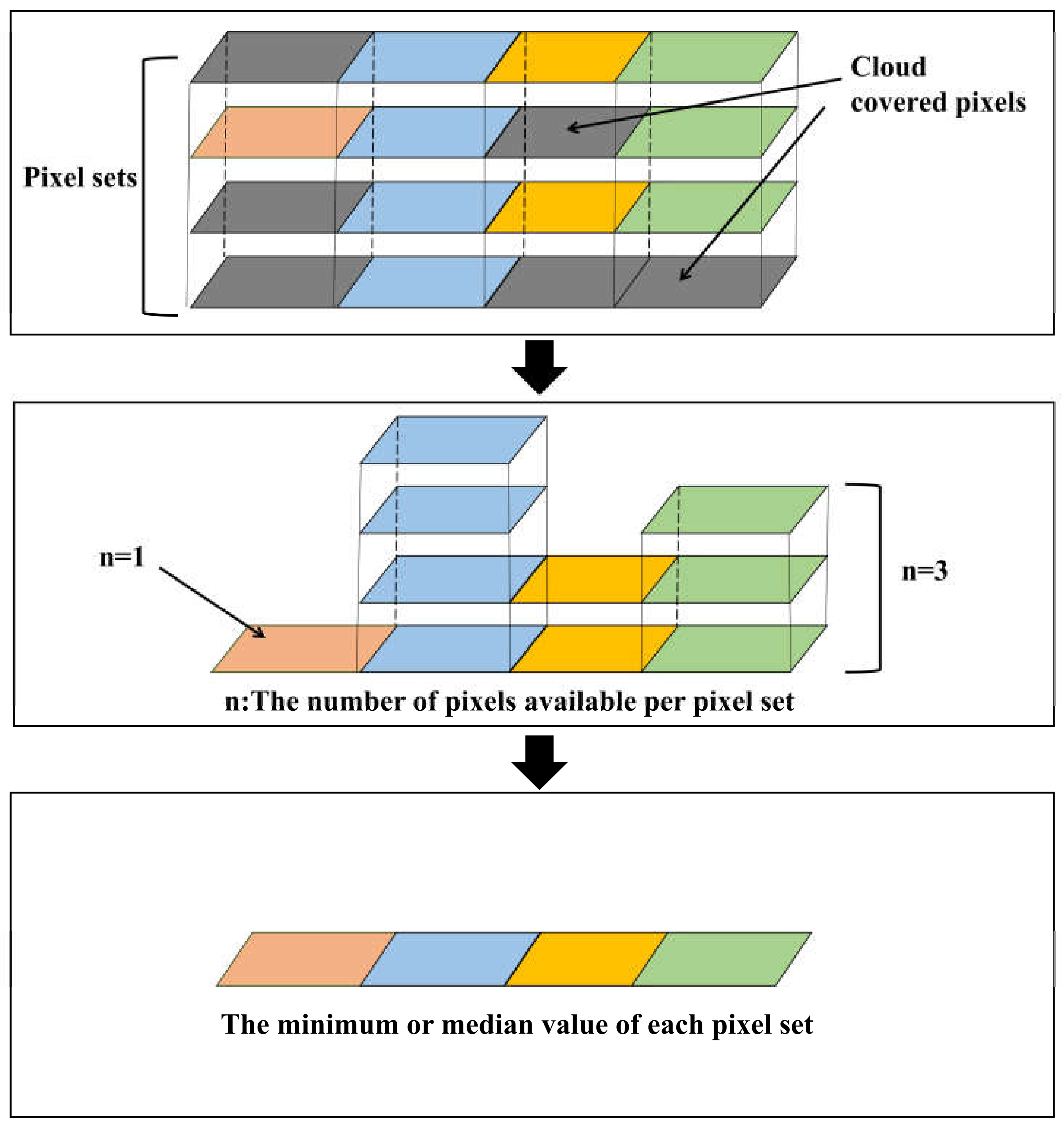
In this study, the Landsat images used were orthorectified in GEE. The overlapping data at each pixel position formed a pixel set. Usually, the minimum or median of pixel sets is used to synthesize images [40,41,52]. The image synthesis process is shown in Figure 3, followed by image collection, cloud filtering, and image synthesis. The spectral characteristics of snow cover are very similar to those of clean glaciers, but vary from those of debris-covered glaciers. Hence, we performed a minimum synthesis of the image set to minimize the influence of snow cover on the first glacier extraction, and then median synthesis of the image set was carried out to enhance the difference between the debris-covered glaciers and the surrounding rocks, which was beneficial in extracting the debris-covered glaciers. Thus, two complete composite images of the study area were formed.

3.2. Feature Construction

3.2.1. Spectral Features

(1)
Common spectral features
Spectral features used in this study were mainly derived from synthetic images, including the first to seventh bands and several indices obtained from various combinations of these bands. These spectral indices included the normalized difference vegetation index (NDVI), normalized difference water index (NDWI), and normalized difference snow cover index (NDSI), which were calculated as follows:
NDVI   = ρ Red ρ NIR ρ Red + ρ NIR ,
NDWI   = ρ Green ρ NIR ρ Green + ρ NIR ,
NDSI   = ρ Green ρ SWIR 1 ρ Green + ρ SWIR 1 ,
where ρ Green , ρ Red , ρ NIR and ρ SWIR 1 are the reflectance values of the Landsat 8 OLI images in the green, red, near-infrared (NIR), and short-wave infrared (SWIR1) bands, respectively.
(2)
Spectral features of glaciers under the influences of shadow and snow cover
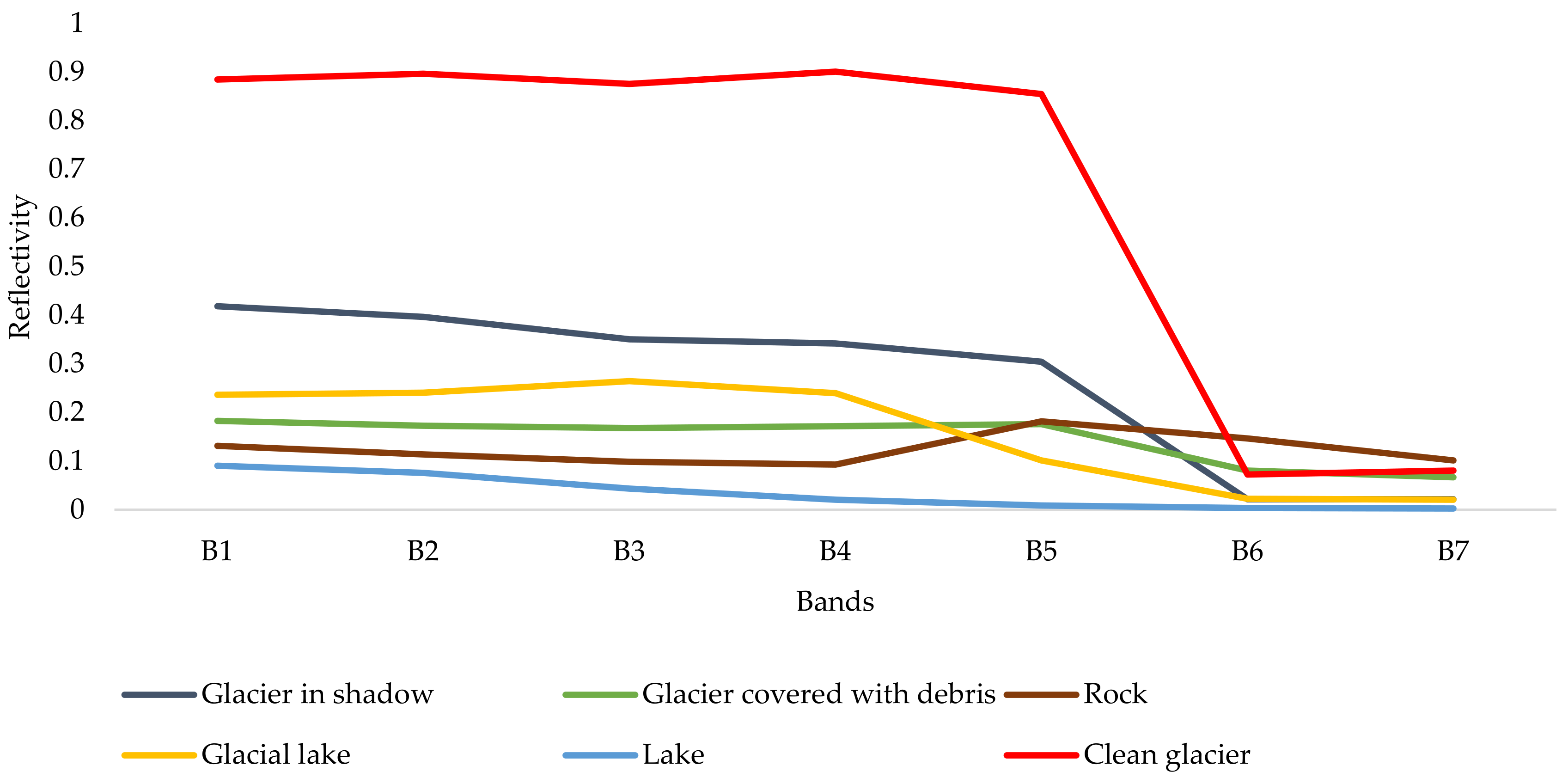
To distinguish the glaciers in shadow, debris-covered glaciers, rocks, glacial lakes, and other objects with similar spectral information, the Landsat 8 TOA image was used to sample glaciers, debris-covered glaciers, rocks, glacial lakes, lakes, and glaciers in shadow on the Tibetan Plateau (Figure 4), and the average reflectance was calculated (Figure 5). Studies have shown that it is easy to distinguish clean glaciers by using the “band ratio”, which is the ratio of the red band (B4) and shortwave infrared band (B6) of Landsat 8 OLI images. However, the traditional band ratio method is easily affected by snow [8], so this study proposed a multi-temporal minimum band ratio index; that is, the ratio of red band (B4) to short wave infrared band (B6) of each pixel of each image was calculated based on the original Landsat 8 dataset, and the new image was synthesized with the minimum band ratio of each pixel point set. More specifically, over a period of time, a non-glacier pixel may be covered by snow many times, but once the surface is exposed, this pixel is regarded as a non-glacier pixel. This index can help reduce the influence of snow on glacier extraction.
After removing the clean glaciers, the spectral features of the remaining glaciers in shadow, the debris-covered glaciers, the rocks, and the glacial lakes were very similar. The band ratio could aid in distinguishing the glaciers in shadow and glacial lakes from other categories (Figure 5). The glaciers in shadow and glacial lakes had a large difference in the near-infrared band (B5), but there was almost no difference in the short-wave infrared band (B6). Therefore, we proposed a “band difference” index (B5–B6) to distinguish the glaciers in shadow and glacial lakes.
(3)
Spectral features of debris-covered glaciers
The spectral features of the remaining debris-covered glaciers and rocks were also very similar. Studies have shown that optical images using thermal radiation technology can improve the extraction accuracy of such glaciers [51]. Therefore, the thermal infrared band (B10) was used in this study.
In the median composite image, the brightness of the debris-covered glaciers, surrounding rocks, and snow considerably varied. To effectively distinguish them, a tasseled cap transformation was performed on the composite image to obtain the brightness, greenness, and humidity information of the pixels.

3.2.2. Texture Features

The effect of glacier extraction relying only on spectral features is not ideal; there can be missing data and misclassifications among different types, because there is a phenomenon of “the same object with different spectrum and different objects with the same spectrum” in remote sensing images [53].
Texture features are visual features that do not depend on color or brightness to reflect the homogeneous phenomenon in an image. These features contain critical information regarding the structure and arrangement of the surface of an object and its relationship with the surrounding environment. The gray-level co-occurrence matrix (GLCM) proposed by Haralick in 1973 [54] is a commonly adopted method for describing texture by studying the spatial correlation characteristics of gray levels. GEE provides a function called glcmTexture to rapidly calculate texture features based on GLCM. In this study, the band ratio of the composite image was used to calculate texture features, including angle second moment, contrast, correlation, variance, inverse different moment, and entropy.

3.2.3. Topographic Features

SRTMGL1_003 data were utilized to derive the elevation, slope, and aspect features. Topographic features were calculated by the function ee.Terrain.products().
Table 2 presents the 25 features constructed in this study.

3.3. Feature Selection

There are numerous features available for classification. If too many features are sent to the classifier for training, it will not only complicate the operation and greatly reduce the processing speed but also decrease the classification accuracy in the case of limited samples. This is called “dimension disaster” [55,56]. Therefore, the selection of significant features plays an important role in remote sensing image classification.
The GEE provides the feature importance analysis method explain(). This method can quickly calculate the importance of features, which is usually consistent with the ranking importance measurements. Therefore, it is necessary to calculate the importance scores of the constructed features, then sort the constructed features according to the importance scores and select the features with higher importance scores for classification.

3.4. Random Forest Classification

3.4.1. Random Forest Parameter Settings

Random forest (RF) is a collection of classification trees proposed by Breiman [57]. The advantages of RF enable it to deal with complex remote sensing image classification and apply to multi-category and multi-feature classification.
The construction of the RF classifier model requires multiple parameters, including the number of decision trees (N) and the number of variables used to split the data (M). Generally speaking, if the value of N is too small, underfitting may occur; if the value of N is too large, it may cause too many calculations. Therefore, it is important to determine an appropriate parameter value. In addition, RF with a large value of M will result in over-surplus calculation for classification. The value of M is typically determined by taking the square root of the number of input variables [58].

3.4.2. Sample Selection

In this study, glaciers, lakes, and others were selected for the first classification, and snow, debris-covered glaciers, water bodies, and others were selected for the second classification. In accordance with the principle of randomness and uniformity, sample points were selected covering the entire study region.

3.4.3. Post-Classification Processing

In the classification results of supervised classification, the band ratio method, or decision tree, there will inevitably be some small pixel patches, which is a common problem of pixel classification, and it will result in adverse effects on image quality and accuracy [59]. Therefore, it is necessary to eliminate or reclassify these small pixel patches.

3.4.4. Accuracy Verification

When collecting samples, we selected approximately 70% as training samples and approximately 30% as verification samples. Based on these verification samples, the commonly used precision evaluation indexes of overall accuracy and Kappa coefficient were used to evaluate the extraction effect of glaciers [60].

3.5. Comparison and Analysis with Glacier Dataset

To show the real performance of the method, it is necessary to compare the glacier extraction results with real glacier datasets and calculate their area differences, including the percentage of correctly extracted glacier area in the total area of glacier dataset (PGD) and the percentage of correctly extracted glacier area in the total area of extracted glacier (PGE). Obviously, the effect of glacier extraction cannot depend solely on PGD or PGE. Only when PGD and PGE are high at the same time can the effect of glacier extraction be very good. Therefore, the harmonic mean (HM) of PGD and PGE was introduced in this study. The higher the HM value, the better the glacier extraction result. The calculation formula is as follows:
HM   = 2 × PGD × PGE PGD + PGE

4. Results and Analysis

4.1. Automatic Extraction of Glaciers on the Tibetan Plateau

4.1.1. The Result of Pre-Processing

In the pre-processing, summer images of the Tibetan Plateau from August to October for the years 2016 to 2020 were selected for this study, which not only ensured enough cloud-free images to cover the study area but also reduced the influence of snow cover.
Owing to the complex terrain of the Tibetan Plateau, many areas are covered by clouds throughout the year. Therefore, it is difficult to synthesize a complete image using only pixels with zero cloud scores. Based on the analysis, we found that the ice and snow pixels covered by thin clouds on the Tibetan Plateau differed from the non-glacial areas, indicating that the possibility of non-glacial pixels being regarded as glacier pixels was very small. Testing different cloud score settings is essential for glacier extraction (Figure 6). Taking the glacier cataloging dataset of western China from 2017 to 2018 as a reference, examples of glacier extraction results were selected for comparison. When the cloud score was set to 40 (Figure 6a), glacier mapping was hardly affected by cloud cover, but there were some missing pixels. When the cloud score was set to 80 (Figure 6c), the area of glaciers that could be extracted was much less than that of the dataset; this may because thick clouds affected the identification of glaciers. When the cloud score threshold was set to 60 (Figure 6b), there was a trade-off between empty pixels and the influence of cloud cover. Therefore, the cloud score threshold used in this study was 60. In extreme cases, the number of pixels used in a pixel set was zero, indicating that there were no remaining pixel sets after the cloud filter. Statistically, the area of empty pixels in the entire study area did not exceed 0.01% of the study area.
After cloud filtering, this study firstly performed a minimum value synthesis of the image set to minimize the influence of snow cover, and then a median synthesis of the image set was carried out to enhance the difference between the debris-covered glaciers and the surrounding rocks. Thus, two complete composite images of the Tibetan Plateau in 2018 were formed.

4.1.2. The Result of Feature Selection

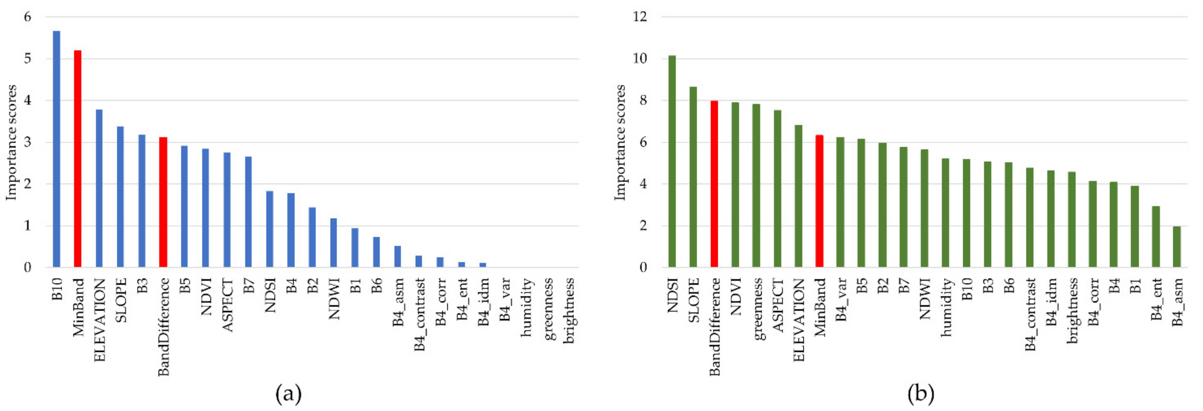
In this study, the importance scores of 25 feature vectors were calculated using the feature importance analysis method provided by GEE (Figure 7). The features were sorted according to the importance scores, and the features with higher importance scores were selected for classification.
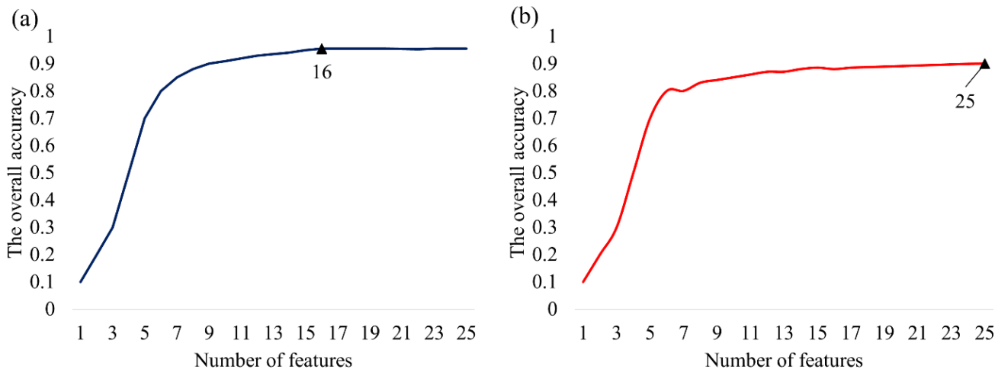
From the above figure, it can be seen that the indexes of band difference (BandDifference) and multi-temporal minimum band ratio (MinBand) constructed in this study were very important for classification. In the two classifications, we selected the top n ( n   ϵ   0 ,   25 ) features with the highest importance score for input and calculated the accuracy (Figure 8). As shown in Figure 8, considering both efficiency and accuracy, when the number of input features was greater than 16 and 25, the classification accuracy did not improve significantly, and the experimental calculation increased. Therefore, the top 16 features and the top 25 features were selected for the first and second classifications, respectively.

4.1.3. Random Forest Classification of Glaciers on the Tibetan Plateau

Within the study region, 861 sample points and 1528 sample points were selected for the first and second classifications, respectively (Table 3). The selection of sample points was based on synthetic images and completed by artificial visual interpretation. To reduce the error caused by human factors, all sample points were selected by one person and verified by another person.
In this study, the number of decision trees (N) was 10, and the number of input features of the two classifiers was 16 and 25; therefore, the values of M were set to 4 and 5, respectively, and the remaining parameters were kept as default values.
After classification, this study filtered the initial results of classification. In the first classification results, we filtered out small pixel patches with less than 30 connected pixels, and in the second classification result, the patches with less than 100 connected pixels were filtered out.

4.1.4. Results of Random Forest Classification

(1)
Glacier extraction result
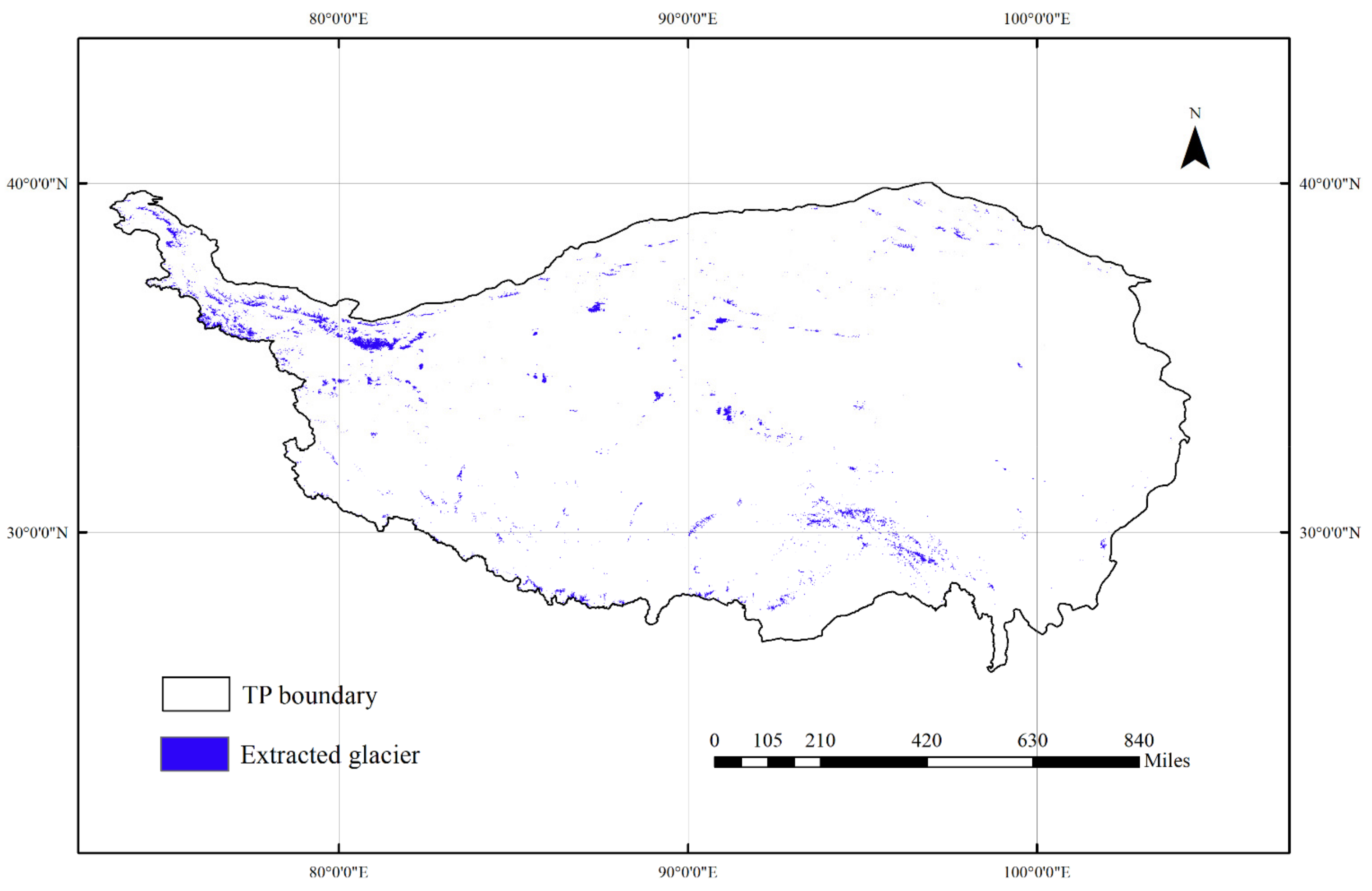
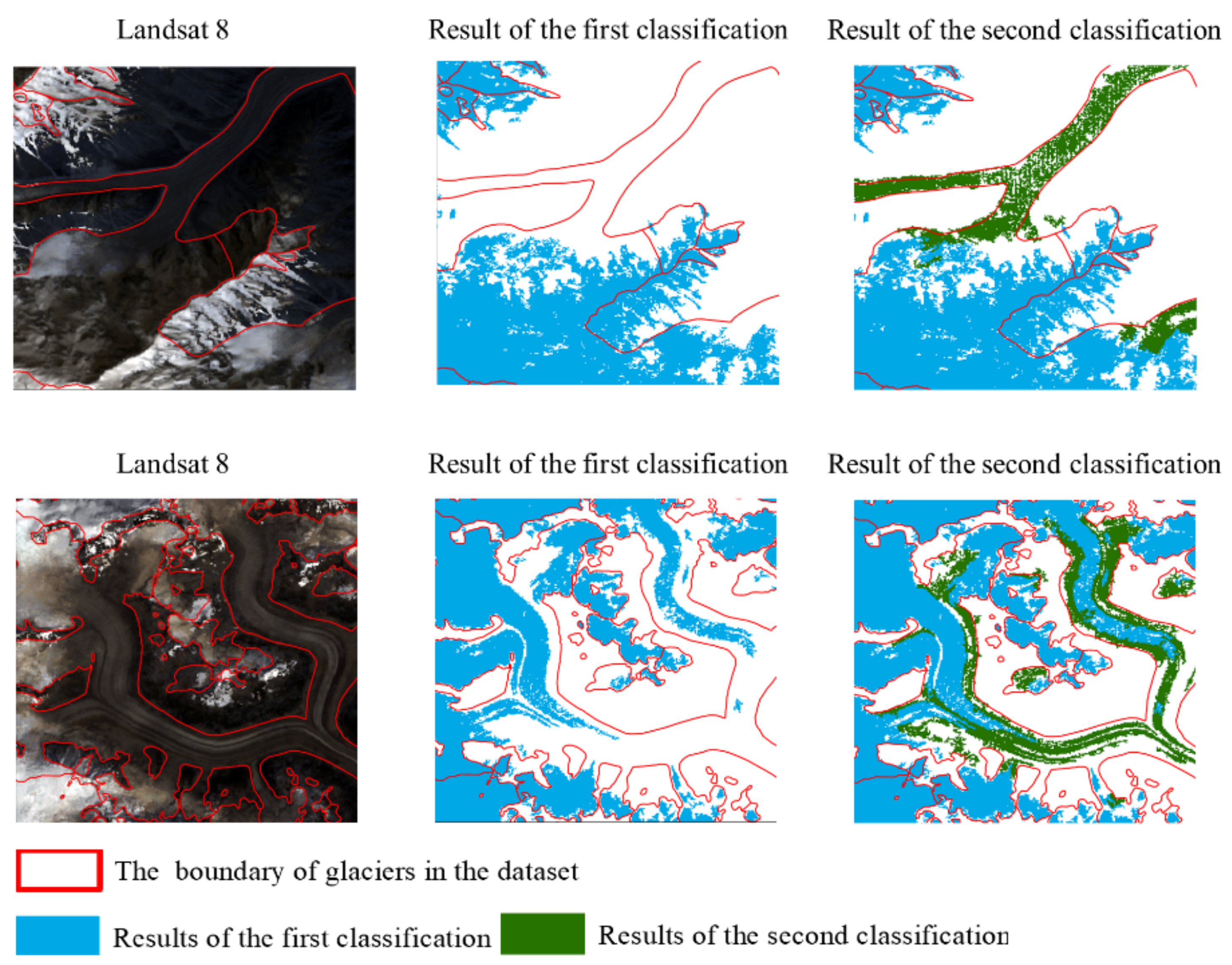
The entire Tibetan Plateau was included in the scope of the study to obtain a complete picture of the glaciers in the region (Figure 9). As the study area was large and the glaciers were relatively small, it was difficult to clearly show all the glacier boundaries. Figure 10 shows the results of some typical glaciers, including the results of the first and second classifications.
(2)
Accuracy verification
Based on the 30% of the sample data, this study calculated the confusion matrices of the results of the first classification and second classification (Table 4 and Table 5). The overall accuracies were 96.04 and 90.75%, and the Kappa coefficients reached 0.92 and 0.83, respectively. The classification results of clean glaciers and glaciers in shadow were slightly better than those of debris-covered glaciers.

4.2. Comparison and Analysis with Glacier Dataset

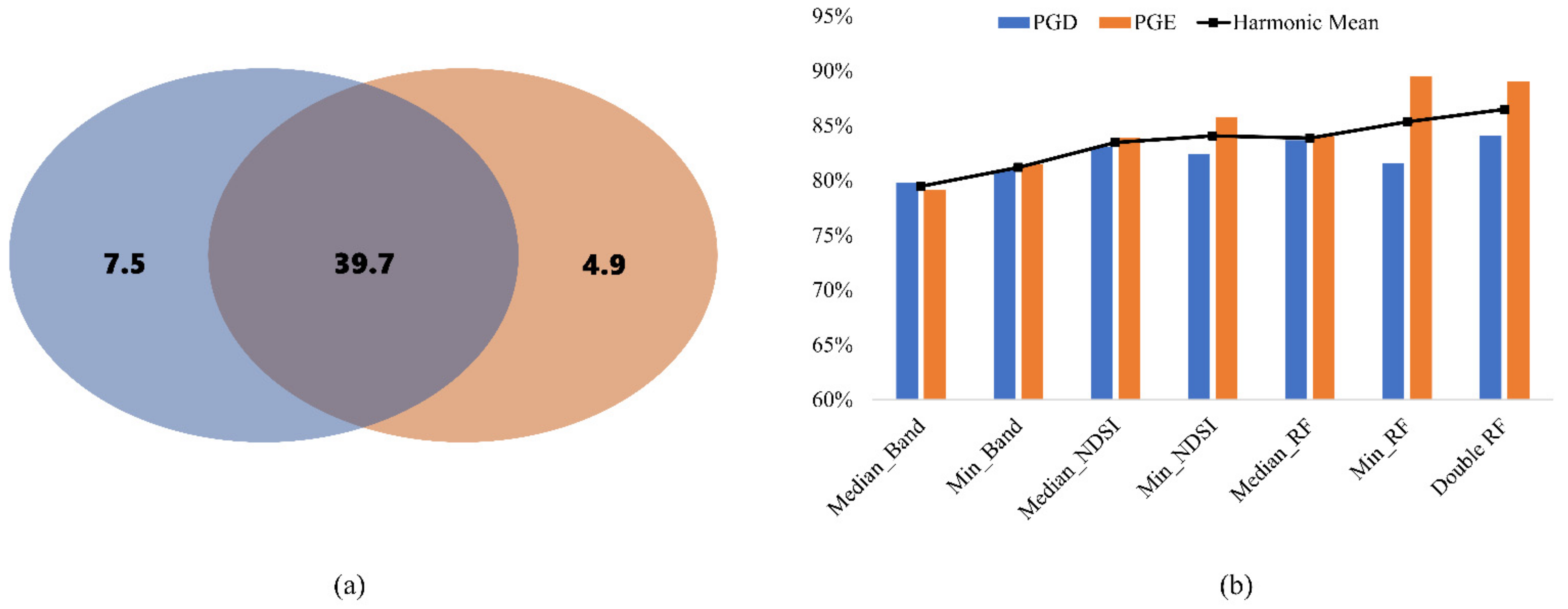
In this study, the classification results obtained by Double RF were compared with the 2017–2018 Glacier Catalogue Dataset in Western China (Figure 11a). Statistically, the glacier area of the glacier dataset was approximately 47,303 km2, the total glacier area of the Tibet Plateau extracted by Double RF was approximately 44,653 km2, and the correctly extracted area was approximately 39,766 km2.
To test the performance of the Double RF method, this study adopted different methods to extract glaciers on the Tibetan Plateau. The band ratio method [8], NDSI method [6], and RF method [9,10] are commonly used in glacier extraction. In this study, the three methods were used for the widely used median composite image and minimum composite image [40,41,52]. There were six methods in total: the band ratio method based on median composite image (Median_Band) (B4/B6 > 5.0), the band ratio method based on minimum composite image (B4/B6 > 5.0), the NDSI method based on median composite image (Median_NDSI) (NDSI > 0.4, NDWI < 0.3), the NDSI method based on minimum composite image (Min_NDSI) (NDSI > 0.4, NDWI < 0.6), the RF method based on median composite image (Median_RF), and the RF method based on minimum composite image (Min_RF). According to previous studies, the NDSI value of snow and ice in Landsat images is greater than 0.4 [61,62], so the NDSI threshold value of this study was set to 0.4, while the NDWI threshold value and B4/B6 threshold value were good results obtained through continuous manual attempts. Therefore, this study used Double RF and six commonly used methods to extract glaciers on the Tibetan Plateau and analyzed the extraction results.
As shown in Figure 11b, the PGD, PGE, and HM of the Double RF method were 84.07%, 89.06%, and 86.49%, respectively. The PGD values of the glacier extraction results of the six commonly used methods, namely Median_Band, Min_Band, Median_NDSI, Min_NDSI, Median_RF, and Min_RF, were 79.78%, 80.93%, 83.05%, 82.42%, 83.69%, and 81.57%, respectively; the PGE values were 79.18%, 81.46%, 83.92%, 85.81%, 84.06%, and 89.53%, respectively; and the HM values were 79.48%, 81.19%, 83.48%, 84.08%, 83.87%, and 85.36%, respectively. Therefore, the HM of the method proposed in this study was the highest, indicating that Double RF results in the best in glacier information extraction, which can achieve high-precision glacier extraction on the Tibetan Plateau.

4.3. Spatial Distribution of Glaciers on the Tibetan Plateau

4.3.1. Glacier Area Distribution

According to the extraction results of the Double RF method proposed by this study, the glacier area of the Tibetan Plateau in 2018 was approximately 44,653 km2, and the area of debris-covered glaciers obtained by the second classification was approximately 750 km2. To clearly determine the distribution characteristics of the glacier scale, the glacier area was divided into five grades [10]: <1 km2, >1 km2 and <5 km2, >5 km2 and <10 km2, >10 km2 and <20 km2, and >20 km2. The number of glaciers in each grade was computed (Figure 12a). According to the result, the number of glaciers with an area of <1 km2 was the greatest, and the number of glaciers with an area >20 km2 was the lowest, accounting for 16.88% and 28.7% of the total area (Figure 12b).

4.3.2. Spatial Distribution Characteristics

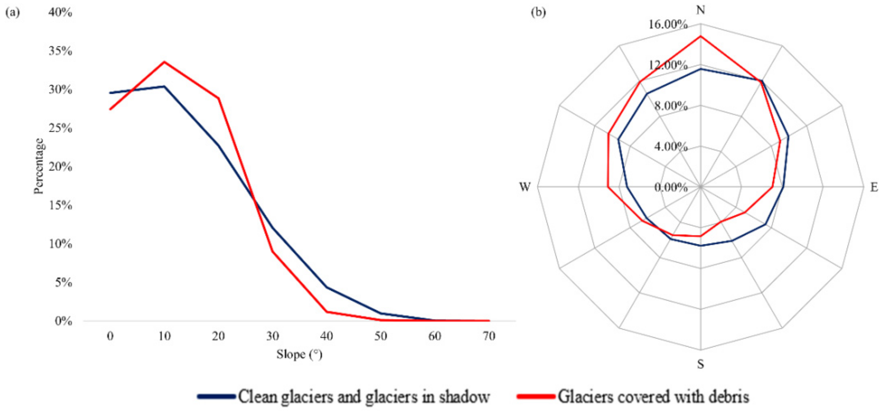
The elevation, slope, and aspect data were calculated from the DEM data (SRTMGL1_003), and they were superimposed with the glacier extraction result data to analyze the spatial distribution characteristics of the glaciers (Figure 13 and Figure 14). To clearly identify the characteristics of the elevation distribution of the debris-covered glaciers, we expanded the area of this part of the glaciers 50-fold (Figure 13b).
When analyzing the distribution characteristics of glaciers at different elevations, it was found that the glacier elevations in the study area showed similar characteristics of a normal distribution. With an increase in altitude, the distribution area of glaciers gradually increased. After the altitude exceeded 5500 m, the distribution area of the glaciers gradually decreased as the altitude continued to increase. In the elevation distribution, the elevation of debris-covered glaciers was lower than that of clean glaciers and glaciers in shadow. The elevations of clean glaciers and glaciers in shadow were mainly distributed between 4500 m and 6500 m, whereas debris-covered glaciers were mainly distributed in the 3500–6000 m range.
The slope of the glaciers in the study area was mainly concentrated in the range from 0–30°, and the number of glaciers in this interval accounted for more than 95%. This was because the slope was too steep and not conducive to the formation of glaciers. The slopes of clean glaciers and glaciers in shadow were mostly less than 50°, whereas the slopes of debris-covered glaciers were mostly less than 40°. This observation provides a reference for distinguishing debris-covered glaciers. In the aspect distribution, all glaciers showed consistency, regardless of whether they were debris-covered glaciers, clean glaciers, or glaciers in shadow; generally, there were fewer glaciers where the slope faces south (180°).

5. Discussion

5.1. Glacier Extraction in Special Areas

Glacier identification is easily affected by shadows, debris, glacial lakes, and so on. For glaciers in alpine areas, remote sensing images usually have large mountain shadows, which cause the amount of information reflected by objects on the ground to be lost or disturbed; the reflectivity of remote sensing image data is low and difficult to interpret in these regions (Figure 5). These shadows include mountain shadows and shadows caused by cloud cover. Studies have shown that supervised classification methods cannot effectively identify glaciers in shadows [63]. Failure to identify glaciers in shadow may lead to erroneous estimates of the glacier contours. In this study, band difference index, traditional band ratio, NDSI, etc., were input into the classifier as feature vectors, and the results were obviously improved, but there were still a few misclassifications. Therefore, it is still an arduous task to identify glaciers in shadow areas in large-scale glacier extraction in alpine regions.
Although the thermal infrared band of optical images can be used to identify debris-covered glaciers [17,18], this is not necessarily applicable to the Tibetan Plateau because of its thick debris coverage [64]. In this study, it was found that it is difficult to extract complete glaciers on a large scale using only RF classification because it is difficult to make a decision when synthesizing an image. If the median synthesis is used, the snow cover will cause confusion. If the minimum synthesis is used, the snow cover is excluded; however, the debris-covered glaciers are difficult to distinguish from surrounding rocks. Therefore, the Double RF method was proposed to extract complete glaciers. The accuracy of extracting debris-covered glaciers on the Tibetan Plateau was over 90%. This method not only weakens the influence of snow but also enhances the difference between the debris-covered glaciers and surrounding rocks. However, this method is still not completely accurate; the accuracy of this method can be improved via manual correction to obtain a more accurate glacier boundary.
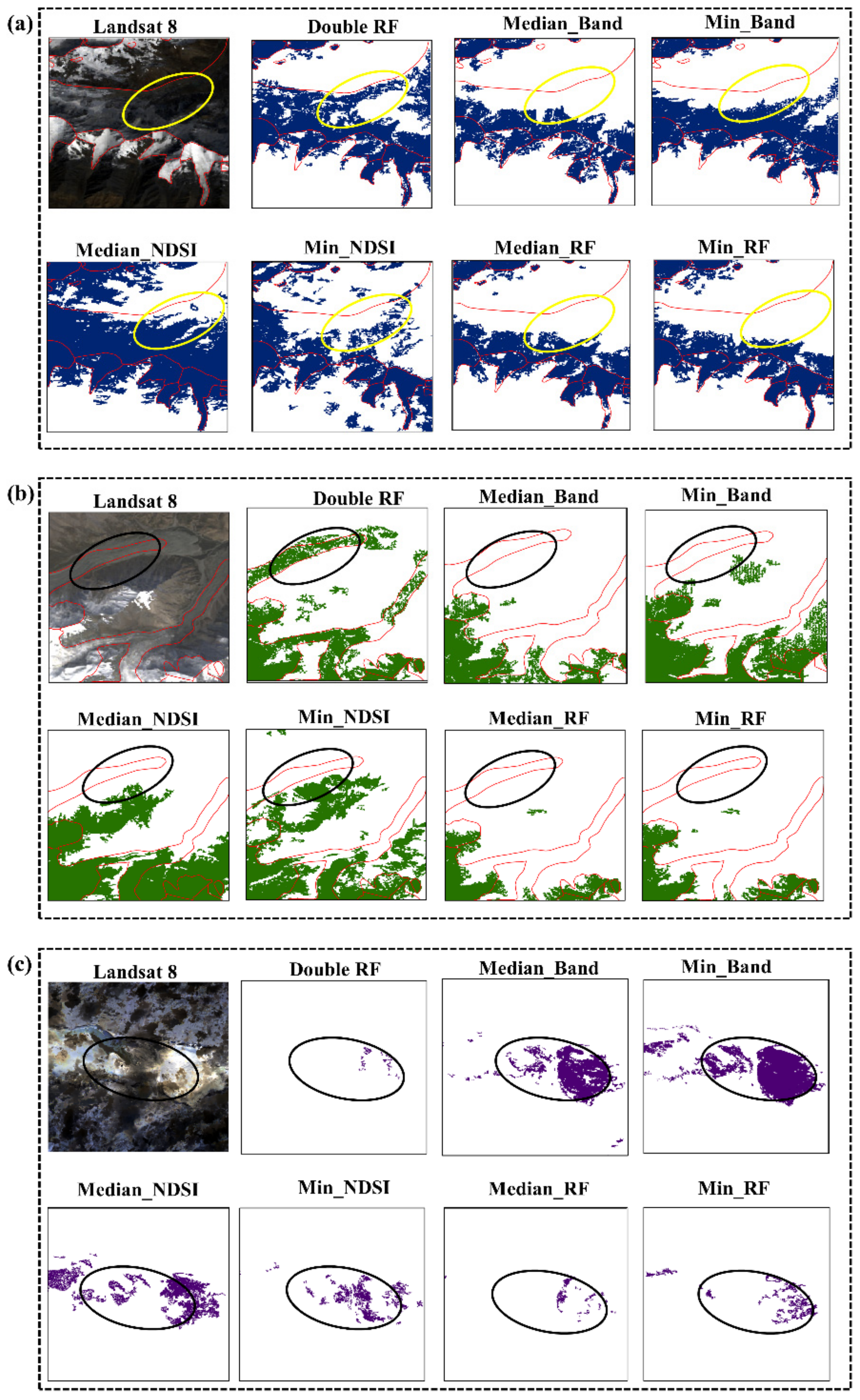
Figure 15 shows the extraction results of seven glacier extraction methods for glaciers in shadow (a), debris-covered glaciers (b), and glacial lakes (c). According to the yellow or black labels, it can be seen that only the Double RF method could effectively extract the debris-covered glacier and avoid the interference of shadow and glacial lakes. None of the other six methods adequately identified these special areas. Among the other six methods, the results of the RF method were better than the band ratio and NDSI method on the whole, because the input features of the RF method in this study were the 25 features we constructed, including the multi-temporal minimum band ratio and band difference index proposed in this study. Even though these methods are very effective for clean glacier extraction, they are all affected by shadows or glacial lakes to varying degrees, and the Double RF method avoids their interference to some extent in the first classification.

5.2. Factors Affecting Classification Accuracy

5.2.1. Selection of Features and Samples

To avoid a dimension disaster, the critical features were selected via the explain() method; however, this may not be the most effective method, because there may be a correlation between the selected features, resulting in information redundancy. Therefore, selecting important features with a low correlation is beneficial for improving the efficiency of the classifier.
Both supervised classification and unsupervised classification need to manually take samples or use other people’s sample datasets. This study selected samples based on artificial visual interpretation. During the sampling process, errors caused by human factors should be avoided as much as possible. To improve the accuracy of the RF classification, high-resolution remote sensing images (high-score series or Sentinel series data) can be used for visual interpretation to obtain accurate sample data.

5.2.2. DEM Accuracy

The DEM accuracy is a key factor that directly affects the topographic features of glaciers. The slope, aspect, and elevation features used in this study were derived from the SRTMGL1_003 DEM data. The situation of the glacier surface and surrounding environment is very complicated, and the 30 m resolution DEM may not reflect the key surface features [18].

5.2.3. Cloud Cover

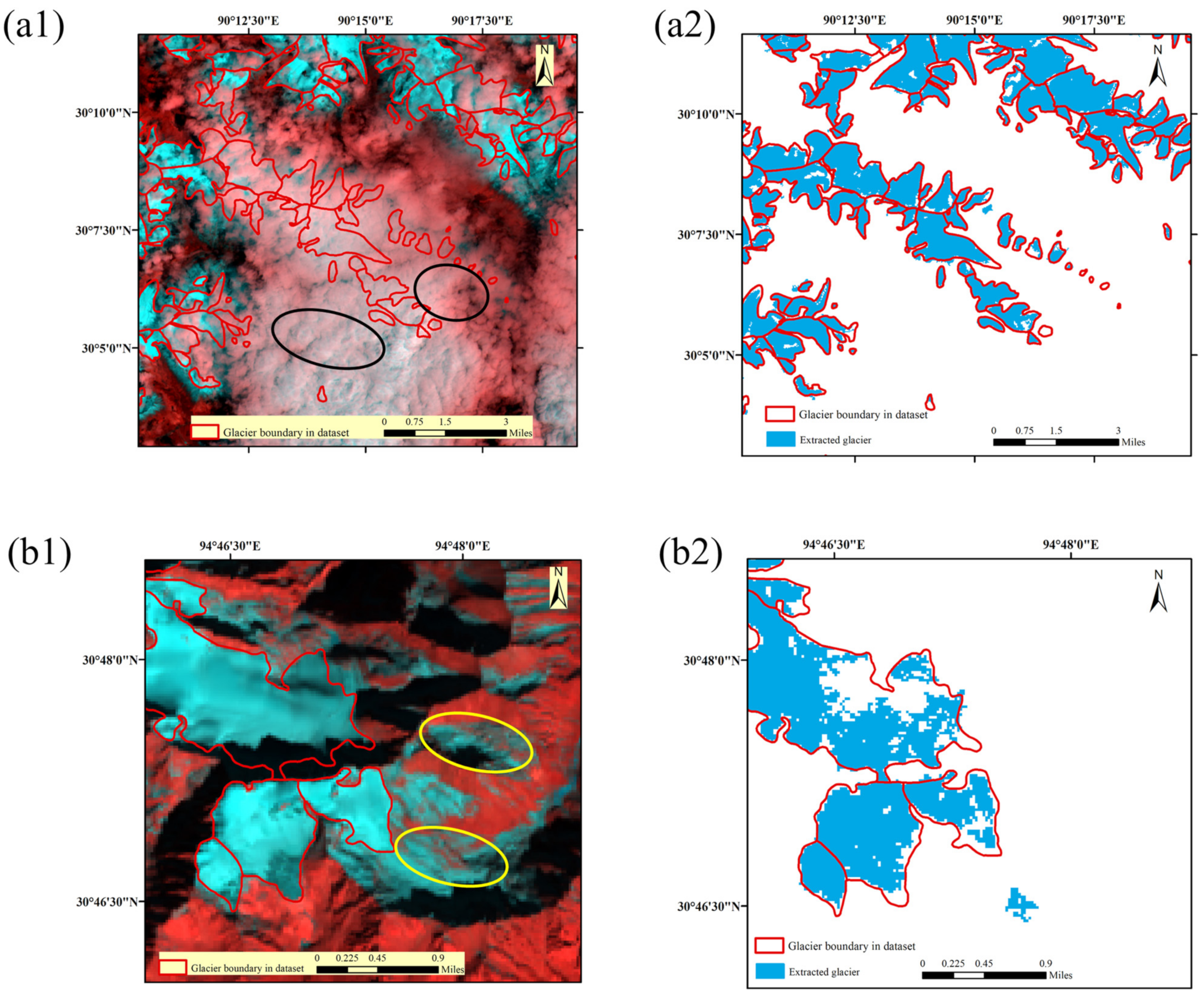
Figure 16(a1) shows the false color composite image of Landsat 8, but there are a large number of white clouds in this area, which makes it difficult to identify glaciers. Even so, the Double RF method proposed in this study achieved a good classification result, which was almost unaffected by clouds (Figure 16(a2)). However, the pixels covered by clouds in the study area were not completely excluded in the experiment. Moreover, in this classification system, the shadow caused by cloud cover could also affect the classification results to a certain extent. In future research, we should pay special attention to the impact analysis of clouds. Microwave data has the ability to penetrate clouds and is not affected them. Therefore, it is possible to consider using microwave data to replace the pixel-by-pixel composite images in future studies.

5.2.4. Snow

In previous studies, physical observation and expert knowledge have aided in identifying glaciers. However, it is difficult to remove seasonal snow from remote sensing satellite images [65]. In this study, we adopted the following measures to reduce the impact of seasonal snow: first, only satellite images in summer were used; second, we input the multi-temporal minimum band ratio index as a classification feature into the RF classifier for classification; third, the minimum synthetic image was used for the first classification to reduce the influence of snow cover. This series of treatments made our work almost unaffected by seasonal snow (Figure 16(b1) and Figure 16(b2)). Even so, permanent snow could not be distinguished by this method, as the spectral features of permanent snow are very similar to those of glaciers, and we could only rely on texture features to assist extraction. Because of these difficulties, it can be seen from this study that the Double RF method is highly suitable for the mapping of glaciers in high mountainous areas.

6. Conclusions

In this study, a new automatic extraction method of glaciers in high-altitude areas was constructed, which reduced the influences of mountain and cloud shadows, cloud coverage, and seasonal snow cover in traditional monitoring, improved the identification accuracy of glaciers in shadows and glaciers covered with debris, and realized full-automatic large-scale glacier mapping.
To accurately realize glacier mapping, this study extracted complete glaciers in two steps: clean glaciers and glaciers in shadow were initially extracted followed by debris-covered glaciers. The detailed steps of glacier extraction include pre-processing, feature construction and selection, classification, and accuracy verification. In the two classifications, we used the minimum composite image and the median composite image, which weakened the influence of snow cover and enhanced the difference between the glacier covered with debris and surrounding rocks. We also proposed two new indexes for random forest classification, namely the reflectivity difference index for identifying glaciers in shadow and glacial lakes and the multi-temporal minimum band ratio index for reducing the influence of snow cover. Finally, we applied this method to the extraction of glaciers on the Tibetan Plateau. The verification results based on 30% sample points showed that the overall accuracies of the first and second classification were 96.04% and 90.75%, respectively, and Kappa coefficients were 0.92 and 0.83, respectively. Compared with the glacier dataset, the PGD, PGE, and HM of the Double RF method were 84.07%, 89.06%, and 86.49%, respectively. These results were obviously superior to the commonly used glacier extraction methods, indicating that this glacier classification method had higher robustness and accuracy.
The Double RF method proposed in this study can be used for future glacier mapping in other alpine regions. The machine-learning classification method has the advantage of being transferable to other regions and datasets. In the future, we will integrate deep learning–based methods into automatic feature extraction, which can reduce the manpower required for manual feature construction and help improve the accuracy of glacier mapping.

Author Contributions

Conceptualization, M.H. and G.Z.; methodology, M.H.; validation, M.H., G.Z. and X.L.; formal analysis, G.Z. and L.Z.; data curation, X.L.; writing—original draft preparation, M.H.; writing—review and editing, G.Z.; funding acquisition, G.Z.; supervision, X.H. and Z.T. All authors have read and agreed to the published version of the manuscript.

Funding

This work was supported by the Second Tibetan Plateau Comprehensive Research Project (2019QZKK0106), National Natural Science Foundation of China (42130514), and Fundamental Research Funds of the Chinese Academy of Meteorological Sciences (2020Z004).

Data Availability Statement

Not applicable.

Acknowledgments

We thank the Google Earth Engine Science team for the freely available cloud-computing platform and USGS for Landsat imagery and SRTM DEM. We thank the glacier dataset provided by Science Data Bank.

Conflicts of Interest

The authors declare no conflict of interest.

References

  1. Cogley, J.G.; Hock, R.; Rasmussen, L.A.; Arendt, A.A.; Bauder, A.; Braithwaite, R.J.; Jansson, P.; Kaser, G.; Möller, M.; Nicholson, L.; et al. Glossary of Glacier Mass Balance and Related Terms; IHP-VII Technical Documents in Hydrology No. 86; IACS Contribution No. 2; UNESCO-IHP: Paris, France, 2011; Available online: https://www.researchgate.net/profile/Lindsey-Nicholson-2/publication/281755921_Glossary_of_glacier_mass_balance_and_related_terms/links/56e6a37308ae65dd4cc1b560/Glossary-of-glacier-mass-balance-and-related-terms.pdf (accessed on 1 June 2022).
  2. Liu, X.; Chen, B. Climatic warming in the Tibetan Plateau during recent decades. Int. J. Climatol. A J. R. Meteorol. Soc. 2000, 20, 1729–1742. [Google Scholar] [CrossRef]
  3. Tian, H.; Yang, T.; Liu, Q. An empirical model to predict glacier area changes in China. IOP Conf. Ser. Earth Environ. Sci. 2019, 349, 012015. [Google Scholar] [CrossRef] [Green Version]
  4. Yao, T.; Pu, J.; Lu, A.; Wang, Y.; Yu, W. Recent glacial retreat and its impact on hydrological processes on the Tibetan Plateau, China, and surrounding regions. Arct. Antarct. Alp. Res. 2007, 39, 642–650. [Google Scholar] [CrossRef] [Green Version]
  5. Paul, F.; Barrand, N.E.; Baumann, S.; Berthier, E.; Bolch, T.; Casey, K.; Frey, H.; Joshi, S.; Konovalov, V.; Le Bris, R. On the accuracy of glacier outlines derived from remote-sensing data. Ann. Glaciol. 2013, 54, 171–182. [Google Scholar] [CrossRef] [Green Version]
  6. Kulkarni, A.; Srinivasulu, J.; Manjul, S.; Mathur, P. Field based spectral reflectance studies to develop NDSI method for snow cover monitoring. J. Indian Soc. Remote Sens. 2002, 30, 73–80. [Google Scholar] [CrossRef]
  7. Sibandze, P.; Mhangara, P.; Odindi, J.; Kganyago, M. A comparison of Normalised Difference Snow Index (NDSI) and Normalised Difference Principal Component Snow Index (NDPCSI) techniques in distinguishing snow from related land cover types. S. Afr. J. Geomat. 2014, 3, 197–209. [Google Scholar] [CrossRef] [Green Version]
  8. Zhang, M.; Wang, X.; Shi, C.; Yan, D. Automated Glacier Extraction Index by Optimization of Red/SWIR and NIR/SWIR Ratio Index for Glacier Mapping Using Landsat Imagery. Water 2019, 11, 1223. [Google Scholar] [CrossRef] [Green Version]
  9. Khan, A.A.; Jamil, A.; Hussain, D.; Taj, M.; Jabeen, G.; Malik, M.K. Machine-learning algorithms for mapping debris-covered glaciers: The Hunza Basin case study. IEEE Access 2020, 8, 12725–12734. [Google Scholar] [CrossRef]
  10. Lu, Y.; Zhang, Z.; Huang, D. Glacier Mapping Based on Random Forest Algorithm: A Case Study over the Eastern Pamir. Water 2020, 12, 3231. [Google Scholar] [CrossRef]
  11. Robson, B.A.; Nuth, C.; Dahl, S.O.; Hölbling, D.; Strozzi, T.; Nielsen, P.R. Automated classification of debris-covered glaciers combining optical, SAR and topographic data in an object-based environment. Remote Sens. Environ. 2015, 170, 372–387. [Google Scholar] [CrossRef] [Green Version]
  12. Bennett, M.M.; Glasser, N.F. Glacial Geology: Ice Sheets and Landforms; John Wiley & Sons: Hoboken, NJ, USA, 2011. [Google Scholar]
  13. Paul, F.; Huggel, C.; Kääb, A. Combining satellite multispectral image data and a digital elevation model for mapping debris-covered glaciers. Remote Sens. Environ. 2004, 89, 510–518. [Google Scholar] [CrossRef]
  14. Frey, H.; Paul, F. On the suitability of the SRTM DEM and ASTER GDEM for the compilation of topographic parameters in glacier inventories. Int. J. Appl. Earth Obs. Geoinf. 2012, 18, 480–490. [Google Scholar] [CrossRef]
  15. Patel, A.; Prajapati, R.; Dharpure, J.K.; Mani, S.; Chauhan, D. Mapping and monitoring of glacier areal changes using multispectral and elevation data: A case study over Chhota-Shigri glacier. Earth Sci. Inform. 2019, 12, 489–499. [Google Scholar] [CrossRef]
  16. Bolch, T.; Buchroithner, M.F.; Kunert, A.; Kamp, U. Automated delineation of debris-covered glaciers based on ASTER data. In GeoInformation in Europe, Proceedings of the 27th Annual Symposium European Association of Remote Sensing Laboratories (EARSeL), Bolzano, Italy, 4–7 June 2007; Millpress: Rotterdam, The Netherlands, 2007; pp. 4–6. [Google Scholar]
  17. Singh, V.; Goyal, M.K. An improved coupled framework for Glacier classification: An integration of optical and thermal infrared remote-sensing bands. Int. J. Remote Sens. 2018, 39, 6864–6892. [Google Scholar] [CrossRef]
  18. Taschner, S.; Ranzi, R. Comparing the opportunities of Landsat-TM and Aster data for monitoring a debris covered glacier in the Italian Alps within the GLIMS project. In Proceedings of the IEEE International Geoscience and Remote Sensing Symposium, Toronto, ON, Canada, 24–28 June 2002; pp. 1044–1046. [Google Scholar]
  19. Smith, T.; Bookhagen, B.; Cannon, F. Improving Semi-Automated Glacier Mapping with a Multi-Method Approach: Applications in Central Asia. Cryosphere 2015, 9, 1747–1759. [Google Scholar] [CrossRef] [Green Version]
  20. Janke, J.R.; Bellisario, A.C.; Ferrando, F.A. Classification of debris-covered glaciers and rock glaciers in the Andes of central Chile. Geomorphology 2015, 241, 98–121. [Google Scholar] [CrossRef]
  21. Lippl, S.; Vijay, S.; Braun, M. Automatic delineation of debris-covered glaciers using InSAR coherence derived from X-, C-and L-band radar data: A case study of Yazgyl Glacier. J. Glaciol. 2018, 64, 811–821. [Google Scholar] [CrossRef] [Green Version]
  22. Racoviteanu, A.; Williams, M.W. Decision tree and texture analysis for mapping debris-covered glaciers in the Kangchenjunga area, Eastern Himalaya. Remote Sens. 2012, 4, 3078–3109. [Google Scholar] [CrossRef] [Green Version]
  23. Nuimura, T.; Sakai, A.; Taniguchi, K.; Nagai, H.; Lamsal, D.; Tsutaki, S.; Kozawa, A.; Hoshina, Y.; Takenaka, S.; Omiya, S. The GAMDAM glacier inventory: A quality-controlled inventory of Asian glaciers. Cryosphere 2015, 9, 849–864. [Google Scholar] [CrossRef] [Green Version]
  24. Zhu, Z.; Woodcock, C.E. Object-based cloud and cloud shadow detection in Landsat imagery. Remote Sens. Environ. 2012, 118, 83–94. [Google Scholar] [CrossRef]
  25. Gorelick, N.; Hancher, M.; Dixon, M.; Ilyushchenko, S.; Thau, D.; Moore, R. Google Earth Engine: Planetary-scale geospatial analysis for everyone. Remote Sens. Environ. 2017, 202, 18–27. [Google Scholar] [CrossRef]
  26. Hird, J.N.; Kariyeva, J.; McDermid, G.J. Satellite Time Series and Google Earth Engine Democratize the Process of Forest-Recovery Monitoring over Large Areas. Remote Sens. 2021, 13, 4745. [Google Scholar] [CrossRef]
  27. Brovelli, M.A.; Sun, Y.; Yordanov, V. Monitoring forest change in the amazon using multi-temporal remote sensing data and machine learning classification on Google Earth Engine. ISPRS Int. J. Geo-Inf. 2020, 9, 580. [Google Scholar] [CrossRef]
  28. Koskinen, J.; Leinonen, U.; Vollrath, A.; Ortmann, A.; Lindquist, E.; D’Annunzio, R.; Pekkarinen, A.; Kayhko, N. Participatory mapping of forest plantations with Open Foris and Google Earth Engine. ISPRS J. Photogramm. Remote Sens. 2019, 148, 63–74. [Google Scholar] [CrossRef]
  29. Chen, B.; Xiao, X.; Li, X.; Pan, L.; Doughty, R.; Ma, J.; Dong, J.; Qin, Y.; Zhao, B.; Wu, Z. A mangrove forest map of China in 2015: Analysis of time series Landsat 7/8 and Sentinel-1A imagery in Google Earth Engine cloud computing platform. ISPRS J. Photogramm. Remote Sens. 2017, 131, 104–120. [Google Scholar] [CrossRef]
  30. Deng, Y.; Jiang, W.; Tang, Z.; Ling, Z.; Wu, Z. Long-Term Changes of Open-Surface Water Bodies in the Yangtze River Basin Based on the Google Earth Engine Cloud Platform. Remote Sens. 2019, 11, 2213. [Google Scholar] [CrossRef] [Green Version]
  31. Mahdianpari, M.; Salehi, B.; Mohammadimanesh, F.; Homayouni, S.; Gill, E. The First Wetland Inventory Map of Newfoundland at a Spatial Resolution of 10 m Using Sentinel-1 and Sentinel-2 Data on the Google Earth Engine Cloud Computing Platform. Remote Sens. 2019, 11, 43. [Google Scholar] [CrossRef] [Green Version]
  32. Liu, X.; Hu, G.; Chen, Y.; Li, X.; Xu, X.; Li, S.; Pei, F.; Wang, S. High-resolution multi-temporal mapping of global urban land using Landsat images based on the Google Earth Engine Platform. Remote Sens. Environ. 2018, 209, 227–239. [Google Scholar] [CrossRef]
  33. Wang, Y.; Li, Z.; Zeng, C.; Xia, G.; Shen, H. An urban water extraction method combining deep learning and google earth engine. IEEE J. Sel. Top. Appl. Earth Obs. Remote Sens. 2020, 13, 769–782. [Google Scholar] [CrossRef]
  34. Tang, Z.; Deng, G.; Li, S.; Li, C.; Chen, H.; Peng, H. Study on the Spatiotemporal Variation of Impervious Surface in Hunan Province for Nearly 30 Years Based on Google Earth Engine. Geogr. Geo-Inf. Sci. 2020, 36, 41–46. [Google Scholar] [CrossRef]
  35. Amani, M.; Mahdavi, S.; Afshar, M.; Brisco, B.; Huang, W.; Mohammad Javad Mirzadeh, S.; White, L.; Banks, S.; Montgomery, J.; Hopkinson, C. Canadian wetland inventory using Google Earth Engine: The first map and preliminary results. Remote Sens. 2019, 11, 842. [Google Scholar] [CrossRef] [Green Version]
  36. Sazib, N.; Mladenova, I.; Bolten, J. Leveraging the Google Earth Engine for drought assessment using global soil moisture data. Remote Sens. 2018, 10, 1265. [Google Scholar] [CrossRef] [PubMed] [Green Version]
  37. Chen, W.; Huang, H.; Tian, Y.; Du, Y. Monitoring and Assessment of the Eco-Environment Quality in the Sanjiangyuan Region based on Google Earth Engine. J. Geo-Inf. Sci. 2019, 21, 10. [Google Scholar]
  38. Hu, Y.; Hu, Y. Land Cover Changes and Their Driving Mechanisms in Central Asia from 2001 to 2017 Supported by Google Earth Engine. Remote Sens. 2019, 11, 554. [Google Scholar] [CrossRef] [Green Version]
  39. Tong, S.; Dong, Z.; Zhang, J.; Bao, Y.; Guna, A.; Bao, Y. Spatiotemporal variations of land use/cover changes in Inner Mongolia (China) during 1980–2015. Sustainability 2018, 10, 4730. [Google Scholar] [CrossRef] [Green Version]
  40. Zhang, J.; Jia, L.; Menenti, M.; Zhou, J.; Ren, S. Glacier area and snow cover changes in the range system surrounding tarim from 2000 to 2020 using google earth engine. Remote Sens. 2021, 13, 5117. [Google Scholar] [CrossRef]
  41. Huang, L.; Li, Z.; Zhou, J.M.; Zhang, P. An automatic method for clean glacier and nonseasonal snow area change estimation in High Mountain Asia from 1990 to 2018. Remote Sens. Environ. 2021, 258, 112376. [Google Scholar] [CrossRef]
  42. Xie, F.; Liu, S.; Wu, K.; Zhu, Y.; Gao, Y.; Qi, M.; Duan, S.; Saifullah, M.; Tahir, A.A. Upward Expansion of Supra-Glacial Debris Cover in the Hunza Valley, Karakoram, During 1990~2019. Front. Earth Sci. 2020, 8, 308. [Google Scholar] [CrossRef]
  43. Bevington, A.R.; Menounos, B. Accelerated change in the glaciated environments of western Canada revealed through trend analysis of optical satellite imagery. Remote Sens. Environ. 2022, 270, 112862. [Google Scholar] [CrossRef]
  44. Torabi Poodeh, H.; Yousefi, H.; Samadi, A.; Arshia, A.; Shamsi, Z.; Yarahmadi, Y. Evaluation of Snow Cover Changes Trend Using GEE and TFPW-MK Test (Case Study: Marber Basin-Isfahan). Iran. J. Ecohydrol. 2021, 8, 195–204. [Google Scholar]
  45. Beltramone, G.; Scavuzzo, M.; German, A.; Ferral, A. Wet snow detection in Patagonian Andes with Sentinel-1 SAR temporal series analysis in GEE. In Proceedings of the 2020 IEEE Congreso Bienal de Argentina (ARGENCON), Resistencia, Argentina, 1–4 December 2020; pp. 1–8. [Google Scholar]
  46. Vale, A.B.; Arnold, N.S.; Rees, W.G.; Lea, J.M. Remote Detection of Surge-Related Glacier Terminus Change across High Mountain Asia. Remote Sens. 2021, 13, 1309. [Google Scholar] [CrossRef]
  47. Bohner, J. General climatic controls and topoclimatic variations in Central and High Asia. Boreas 2006, 35, 279–295. [Google Scholar] [CrossRef]
  48. Zhang, Y.; Li, B.; Zheng, D. A discussion on the boundary and area of the Tibetan Plateau in China. Geogr. Res. 2002, 21, 128. [Google Scholar]
  49. Farr, T.G.; Rosen, P.A.; Caro, E.; Crippen, R.; Duren, R.; Hensley, S.; Kobrick, M.; Paller, M.; Rodriguez, E.; Roth, L. The shuttle radar topography mission. Rev. Geophys. 2007, 45, RG2004. [Google Scholar] [CrossRef] [Green Version]
  50. Ran, W.; Wang, X.; Guo, W.; Zhao, H.; Zhao, X.; Liu, S.; Wei, J.; Zhang, Y. A dataset of glacier inventory in Western China during 2017–2018 (V1). Sci. Data Bank 2021. [Google Scholar] [CrossRef]
  51. Wu, M.; Han, Y.; Zhang, D.; Wang, X.; Gesang, W. Information Extraction Method of Debris-Covered Glaciers in Bomi County. Mt. Res. 2017, 35, 238–245. [Google Scholar] [CrossRef]
  52. Kumari, N.; Srivastava, A.; Dumka, U.C. A long-term spatiotemporal analysis of vegetation greenness over the Himalayan Region using Google Earth Engine. Climate 2021, 9, 109. [Google Scholar] [CrossRef]
  53. Jia, K.; Li, Q. Review of Features Selection in Crop Classification Using Remote Sensing Data. Resour. Sci. 2013, 35, 2507–2516. [Google Scholar]
  54. Haralick, R.M.; Shanmugam, K.; Dinstein, I. Textural features for image classification. IEEE Trans. Syst. Man Cybern. 1973, SMC-3, 610–621. [Google Scholar] [CrossRef] [Green Version]
  55. Bach, F. Breaking the curse of dimensionality with convex neural networks. J. Mach. Learn. Res. 2017, 18, 629–681. [Google Scholar]
  56. Kuo, F.Y.; Sloan, I.H. Lifting the curse of dimensionality. Not. AMS 2005, 52, 1320–1328. [Google Scholar]
  57. Breiman, L. Random forests. Mach. Learn. 2001, 45, 5–32. [Google Scholar] [CrossRef] [Green Version]
  58. Gislason, P.O.; Benediktsson, J.A.; Sveinsson, J.R. Random forests for land cover classification. Pattern Recognit. Lett. 2006, 27, 294–300. [Google Scholar] [CrossRef]
  59. Huang, X.; Lu, Q.; Zhang, L.; Plaza, A. New postprocessing methods for remote sensing image classification: A systematic study. IEEE Trans. Geosci. Remote Sens. 2014, 52, 7140–7159. [Google Scholar] [CrossRef]
  60. Zourarakis, D.P. Remote Sensing Handbook–Volume I: Remotely Sensed Data Characterization, Classification, and Accuracies. Photogramm. Eng. Remote Sens. 2018, 84, 481. [Google Scholar] [CrossRef]
  61. Burns, P.; Nolin, A. Using atmospherically-corrected Landsat imagery to measure glacier area change in the Cordillera Blanca, Peru from 1987 to 2010. Remote Sens. Environ. 2014, 140, 165–178. [Google Scholar] [CrossRef] [Green Version]
  62. Scherler, D.; Wulf, H.; Gorelick, N. Global assessment of supraglacial debris-cover extents. Geophys. Res. Lett. 2018, 45, 11,798–11,805. [Google Scholar] [CrossRef] [Green Version]
  63. Ji, X.; Chen, Y.; Luo, X.; Li, Y. Study on the Identification Method of Glacier in Mountain Shadows Based on Landsat 8 OLI Image. Spectrosc. Spectr. Anal. 2018, 38, 3857–3863. [Google Scholar]
  64. Tielidze, L.G.; Bolch, T.; Wheate, R.D.; Kutuzov, S.S.; Lavrentiev, I.I.; Zemp, M. Supra-glacial debris cover changes in the Greater Caucasus from 1986 to 2014. Cryosphere 2020, 14, 585–598. [Google Scholar] [CrossRef] [Green Version]
  65. Sorg, A.; Bolch, T.; Stoffel, M.; Solomina, O.; Beniston, M. Climate change impacts on glaciers and runoff in Tien Shan (Central Asia). Nat. Clim. Chang. 2012, 2, 725–731. [Google Scholar] [CrossRef]
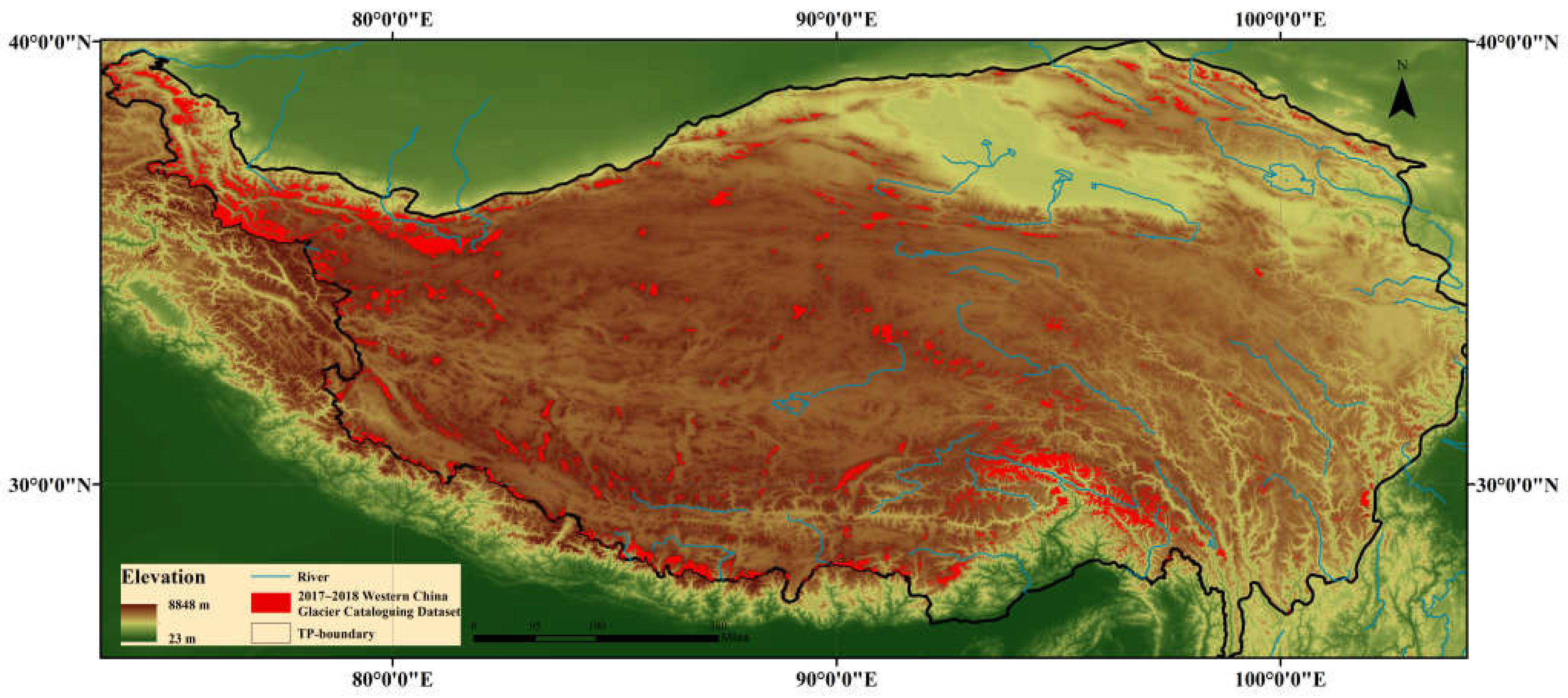
Figure 1. Study region.
Remotesensing 14 03084 g001
Figure 2. The process of glacier extraction.
Remotesensing 14 03084 g002
Figure 3. Image synthesis process.
Remotesensing 14 03084 g003
Figure 4. Sample collection of similar ground objects. (af) indicate shadow glaciers, debris-covered glaciers, rocks, glacial lakes, lakes, and clean glaciers, respectively. The S represents the area of each sampling area.
Remotesensing 14 03084 g004
Figure 5. Average spectral reflectance of different ground objects.
Remotesensing 14 03084 g005
Figure 6. Cloud score threshold setting experiment: the blue area is the extracted glacier, the red line is the glacier boundary of the dataset, and the cloud scores of the three images were set to 40 (a), 60 (b) and 80 (c).
Remotesensing 14 03084 g006
Figure 7. Importance score: (a) is the first classification and (b) is the second classification.
Remotesensing 14 03084 g007
Figure 8. Feature experiment of two classifications: (a) the first classification; (b) the second classification.
Remotesensing 14 03084 g008
Figure 9. Overall glacier extraction results on the Tibetan Plateau.
Remotesensing 14 03084 g009
Figure 10. Details of glacier extraction results on the Tibetan Plateau. The red line is the boundary of glaciers in the dataset.
Remotesensing 14 03084 g010
Figure 11. Comparison of extraction results of different methods. (a) Comparison between the results obtained by the Double RF method and the glacier dataset. The blue part represents the glaciers in the dataset, the yellow part represents the extracted glaciers, and the intersecting part represents the correctly extracted glaciers. The numbers above each part represent the area of the glacier in that part, and the unit is 1000 square kilometers. (b) shows PGD, PGE. and HM for the seven methods.
Remotesensing 14 03084 g011
Figure 12. Statistics of glaciers of different sizes on the Tibetan Plateau: (a) the percentage of the number of glaciers of different sizes; (b) the percentage of the area of glaciers of different sizes.
Remotesensing 14 03084 g012
Figure 13. Elevation distribution of glaciers: (a) the elevation distribution of all glaciers; (b) the elevation distribution of clean glaciers, glaciers in shadow, and debris-covered glaciers.
Remotesensing 14 03084 g013
Figure 14. Percentages of the two types of glaciers at different slopes (a) and different aspects (b).
Remotesensing 14 03084 g014
Figure 15. Extraction results of glaciers in shadow (a), debris-covered glaciers (b), and glacial lakes (c) using seven methods. The red line is the glacier reference boundary of glacier dataset. The parts circled in black or yellow lines are glaciers in shadow, debris-covered glaciers, and glacial lakes.
Remotesensing 14 03084 g015
Figure 16. Influences of cloud cover and snow cover. The black and yellow circles refer to clouds and snow, respectively.
Remotesensing 14 03084 g016
Table 1. The data and sources used in the study.
DataSource
The boundary of the Tibetan PlateauA discussion on the boundary and area of the Tibetan Plateau in China [48]
Landsat image dataUnited States Geological Survey
DEM dataThe Shuttle Radar Topography Mission, SRTM [49]
Glacier catalog datasetA dataset of glacier inventory in Western China during 2017–2018 (V1) [50]
Table 2. Feature construction.
SourceFeature
Spectral featuresComposite imageB1~B7, B10, NDVI, NDWI, NDSI, band difference
Tasseled cap transform imageGreenness, brightness, humidity
Original datasetMulti-temporal minimum band ratio
Texture featuresBand ratio of the composite imageSecond moment, contrast, correlation, variance, inverse different moment, and entropy
Topographic featuresSRTMGL1_ 003Elevation, slope, aspect
Table 3. Type and number of sample points.
First ClassificationSecond Classification
CategoryNo. of samplesCategoryNo. of samples
Glacier181Snow84
Water body126Glacier covered with debris384
Others554Water body180
Others880
Table 4. Results of the first classification verification set.
GlacierWater BodyOthersTotal
Glacier540357
Water body027330
Others31162166
Total5728168253
Table 5. Results of the second classification verification set.
SnowGlacier Covered with DebrisWater BodyOthersTotal
Snow2410328
Glacier covered with debris292021115
Water body0037037
Others0133269285
Total2610640293495
Publisher’s Note: MDPI stays neutral with regard to jurisdictional claims in published maps and institutional affiliations.