Article

Settlement Prediction of Reclaimed Coastal Airports with InSAR Observation: A Case Study of the Xiamen Xiang’an International Airport, China

1
School of Geosciences and Info-Physics, Central South University, Changsha 410083, China
2
Naval Institute of Hydrographic Surveying and Charting, Tianjin 300061, China
3
Fujian Provincial Institute of Land Surveying and Mapping, Xiamen 361006, China
4
Big Data Institute of Digital Natural Disaster Monitoring in Fujian, Xiamen University of Technology, Xiamen 361024, China
*
Author to whom correspondence should be addressed.
Remote Sens. 2022, 14(13), 3081; https://doi.org/10.3390/rs14133081
Submission received: 12 May 2022 / Revised: 13 June 2022 / Accepted: 22 June 2022 / Published: 27 June 2022
(This article belongs to the Special Issue Remote Sensing for Natural Hazards Assessment and Control)

Abstract

:
Many coastal cities reclaim land from the sea to meet the rapidly growing demand for land caused by population growth and economic development. Settlement in reclaimed land may delay construction and even damage infrastructures, so accurately predicting the settlement over reclaimed areas is important. However, the limited settlement observation and ambiguous final settlement estimation affect accurate settlement prediction in traditional methods. This study proposes a new strategy to solve these problems by using the Multitemporal Interferometric Synthetic Aperture Radar (MT-InSAR) method and takes the Xiamen Xiang’an International Airport, built on reclaimed land, as an example. The MT-InSAR is adopted to process the Sentinel-1 images to obtain the settlement history of the study area. The results show that settlement mainly occurs in the reclaimed areas, with the maximum average settlement rate exceeding 40 mm/y. We use the statistical properties of curve fitting to choose the best curve model from several candidate curve models to predict the settlement time series. The Asaoka method is used to identify the critical state between settlement and stability. We predict the consolidation time of the whole study area and reveal that the deformation rate is positively correlated with the consolidation time. The maximum remaining settlement time is over ten years since 24 December 2019. Therefore, manual compaction operations can be carried out to speed up settlement in the areas that need a long time to consolidate. The proposed method can be used to predict the settlement of similar reclaimed areas, and the predicted results can provide a reference for engineering construction.

Graphical Abstract

1. Introduction

Land reclamation from the sea has become an important strategy to promote economic growth and alleviate the population density in coastal areas [1,2,3]. However, the compaction of the underlying soft soil layers in reclaimed areas often leads to land subsidence, which may cause damage to undergoing construction and infrastructures [4,5]. Settlement monitoring and prediction are important in engineering geology [6], especially for reclaimed areas, where the underlying layers are highly compressible and require a long time for consolidation. Moreover, post-construction settlement prediction based on the foundation displacements can provide a reference for engineering construction, deformation early warning, and future land reclamation.
The methods used to predict the settlement include theoretical estimations based on the soil consolidation theory [7] and curve-fitting or prediction models based on deformation measurements [8]. The application of the former is limited by the few samples used and theoretical deviations due to different soil compositions. The latter relies on deformation observations, which are easy to obtain. Therefore, the second group of methods, such as hyperbolic curve [4,9,10], exponential function [11,12,13], and grey model [14,15,16], are well-applied in engineering settlement monitoring and prediction.
Land settlement is often monitored via in situ measurements and remote sensing technology. However, in situ measurements, such as Global Navigation Satellite System (GNSS), leveling, and extensometers, usually have low spatial resolutions due to labor intensity and high cost [17]. Therefore, with in situ measurements, it is difficult to obtain the detailed spatial distribution of deformation, which may lead to misunderstanding settlement behaviors. Interferometric Synthetic Aperture Radar (InSAR) has the ability to obtain the spatial–temporal distribution of deformation with promising accuracy. More importantly, it works in a non-contact style, so the acquisition of those data does not affect engineering construction. Consequently, InSAR has been widely used in measuring ground deformation, such as landslides [18,19,20], tectonic movements [21,22,23], volcano dynamics [24,25], and land subsidence [26,27,28,29], as well as oil and gas fields [30,31]. Moreover, the ability of long-term deformation time series retrieval of multitemporal InSAR (MT-InSAR) enables InSAR to predict the settlement of the reclaimed areas.
For settlement prediction, most studies have chosen prior functional models (e.g., hyperbolic function, Poisson function, exponential function) to predict the total amount and termination time of settlement. Kim et al. [9] introduced the hyperbolic model and persistent scatterer InSAR (PS-InSAR) to monitor the land subsidence in Mokpo City, South Korea. They showed that the prior hyperbolic model has better performance than the linear model. Hu et al. [11] used multisource remote sensing imagery to characterize landscape changes in Yan’an, China. They chose the exponential curve model to predict the consolidation time of the subsiding area. Deng et al. [15] combined PS-InSAR with Grey system theory to monitor and predict land subsidence in the Beijing Plain. The results indicated that this method can be an alternative to conventional numerical and empirical models for short-term prediction in cases in which there is a lack of detailed geological or hydraulic information. The method of combining InSAR with curve models to monitor and predict land subsidence has also been used in different scenarios [4,12,13,32]. Most studies chose curve models based on experience for settlement monitoring and prediction. The selected prior models, however, are likely not suitable to describe the deformation of the studied areas. Shi et al. [17] reported that different models lead to large variations in settlement predictions. They used exponential curve, hyperbolic curve, and quadratic curve to model the settlement time series. However, the quadratic curve failed to predict the settlement. The maximum difference in the final settlement amount predicted by the two curves can reach 0.2 m. In addition, it is not easy to identify the critical state between deformation and stability by the curve-fitting method, resulting in biased predictions of the total amount and the termination time of settlement.
To solve the abovementioned problems, this study proposes a two-step settlement prediction method. In step one, sufficient deformation points provided via MT-InSAR are used to choose the best curve to model the settlement pattern. In step two, the predicted settlement time series and the Asaoka method [33] are used to predict the final settlement amount and consolidation time. The method is validated using the Xiamen Xiang’an International Airport (referred to as XXIA hereafter), China, a reclaimed airport under construction, as a case study.
This study is organized as follows: The study area and datasets are introduced in Section 2. Section 3 describes the processing flow of MT-InSAR and the deformation results of the XXIA. Section 4 describes the procedure of settlement prediction. In Section 5, we discuss the total settlement and the consolidation time of the study area. Some conclusions are drawn in Section 6.

2. Study Area and Datasets
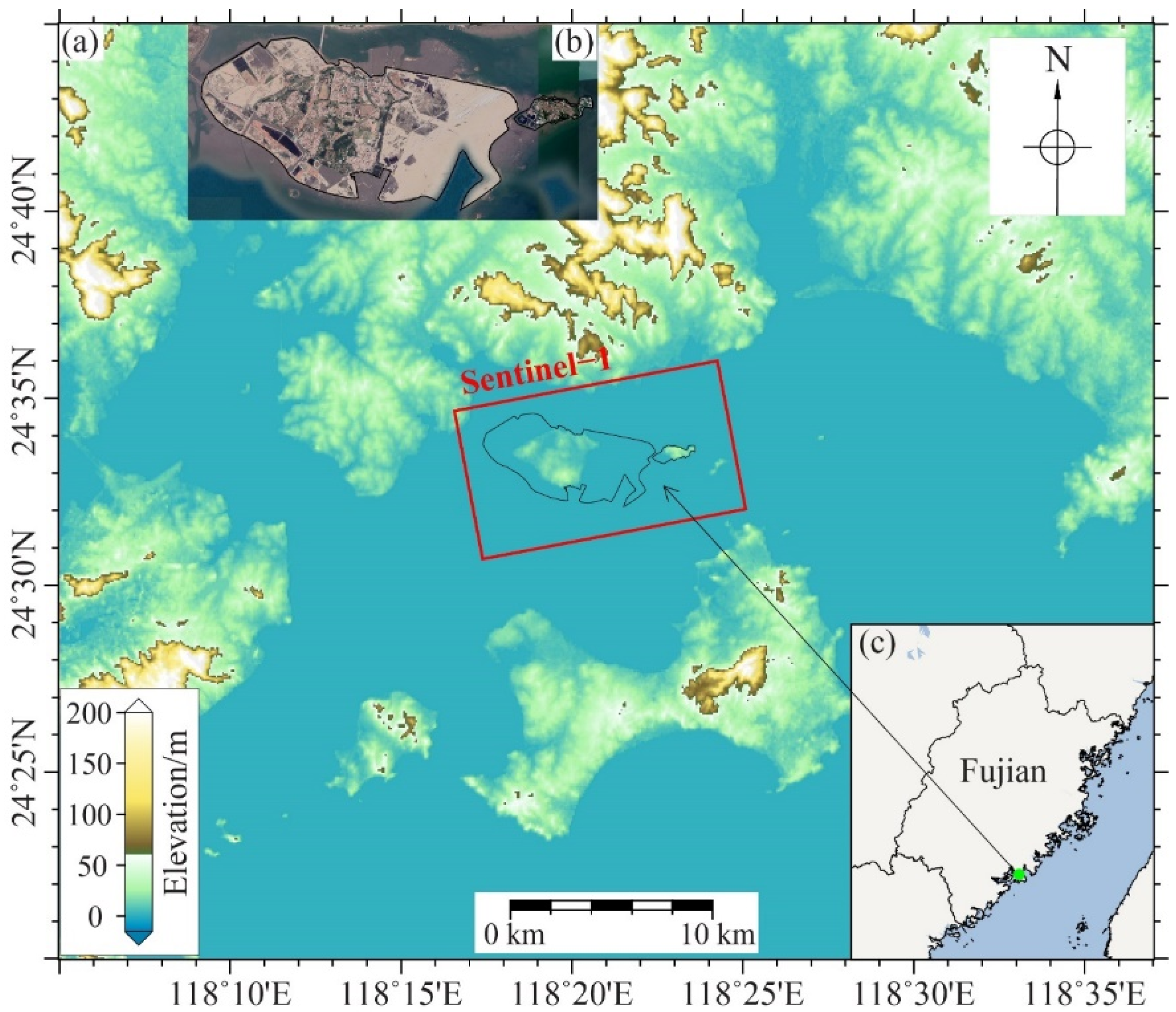
Sentinel-1 images over the XXIA acquired between July 2015 and December 2019 were processed via MT-InSAR to obtain the deformation of the whole study area. Then, we chose the best curve function to model and predicted the deformation time series of the study area. The study area and datasets are described in subsequent sections.

2.1. Study Area

The XXIA, a planned 4F-class international airport, is located in the southeast of Dadeng Island, Xiamen City, China (Figure 1 and Figure 2). The construction of the XXIA started on 4 January 2022, and about 26 km2 of the XXIA will be built on reclaimed land. The land reclamation project of the XXIA has three phases (Figure 2); the first two phases have been completed, after which the reclaimed land experienced settlement [2,34]. Settlement monitoring and prediction of the reclaimed land are crucial to the safe construction of the XXIA. However, predictions of the total settlement amount and consolidation time of the XXIA have not yet been reported.

2.2. Datasets

A total of 128 ascending Sentinel-1 images acquired between 6 July 2015 and 24 December 2019 were collected to obtain the deformation time series of the reclaimed land (Table A1). Coverage of the Sentinel-1 data is shown in Figure 1. The main parameters of the Sentinel-1 images are summarized in Table 1. The images were acquired after the first and second reclamation phases were completed. In addition, the SRTM DEM with a resolution of 30 m was collected to simulate and remove the topographic phase in the differential interferograms.

3. MT-InSAR Processing and Deformation Results

3.1. MT-InSAR Processing

Sentinel-1 SAR images have small perpendicular baselines, so only the temporal baselines were considered selecting interferometric pairs. The maximum temporal baseline was set as 36 days. The interferometric pairs were processed via a multi-look operation (range × azimuth = 5 × 1) to form the interferograms. The SRTM DEM was used to remove the phase contribution of topography in the interferograms. After interferogram filtering and phase unwrapping, the first-order polynomial function model was used to remove the phase ramps. Some areas in the study area were reclaimed from the sea, so they have no external DEM data. We assumed the elevation of the reclaimed land to be 1 and selected high-quality interferograms to perform linear regression between topographic errors and perpendicular baselines to estimate and remove topographic errors. We used the amplitude dispersion of pixels [35], intensity, and coherence to remove poor-quality pixels. The singular value decomposition (SVD) [36] was used to calculate the phase time series of each pixel. We estimated the linear deformation using the least square method and then subtracted the phase contributions of linear deformation from the phase time series. The residual components in the phase time series mainly include nonlinear deformation, atmospheric artifacts, and noise. The atmospheric phases are highly correlated in space, while lowly correlated in time. Noise is lowly correlated in both space and time domains. Therefore, we used temporal and spatial filtering to extract nonlinear deformations from the residual phases. The final deformation time series of each pixel is the sum of linear deformation and nonlinear deformation. The least-square method was performed in the final deformation time series to estimate the average deformation rate of each pixel.

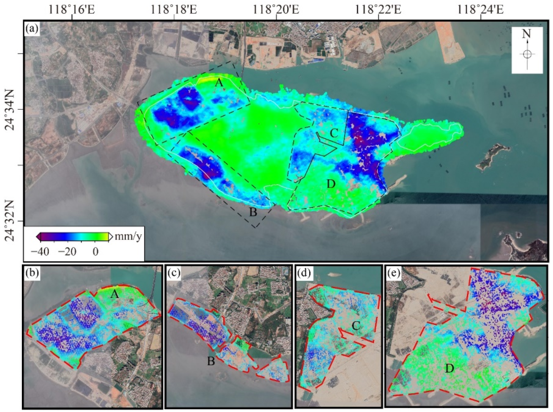
3.2. Deformation Results

Figure 3 shows the average deformation rate in the line-of-sight (LOS) direction of the study area. The selected pixels were sufficient to show the spatial distribution of the settlement, and the deformation areas obtained in this study are generally consistent with the previous studies [2,34], although the monitoring periods were different. Four areas, areas—A, B, C, and D—suffered severe settlement, and the maximum settlement rate exceeded 40 mm/y. The settlement mainly occurred in the reclaimed areas, including the area reclaimed in the first phase (Figure 3d), the second phase (Figure 3e), and the reclaimed areas in the northwest (Figure 3a) and southwest (Figure 3b) of Dadeng Island. The settlement was particularly severe in the northeast of the area reclaimed in the second phase.
The first reclamation phase was completed before July 2015, earlier than the monitoring time of InSAR. According to the soil consolidation theory [7], some points (see Section 4) in area C have finished the primary consolidation and entered the second compression stage. The settlement rate in the area reclaimed in the first stage was around 15 mm/y, with a maximum settlement rate of 20 mm/y. For area C, the maximum settlement rate was observed in the southern part, but some points in this area had become stable after the reclamation. Among the four areas, area C was first reclaimed, so it had the minimum deformation rate, due to the longer time of consolidation. It is possible that areas A, B, and D will have a settlement pattern similar to area C in the time domain, as they had similar strategies of reclamation. Area D had the maximum average settlement rate, as it was reclaimed in the second phase, which was accomplished in March 2018 and has just entered the primary consolidation stage. Inside each area, the settlement rates were different. Specifically, in area D, the southern part was stable, but the northern part experienced serious settlement. One explanation is that this area underwent several reclamations at different times (see Section 5).

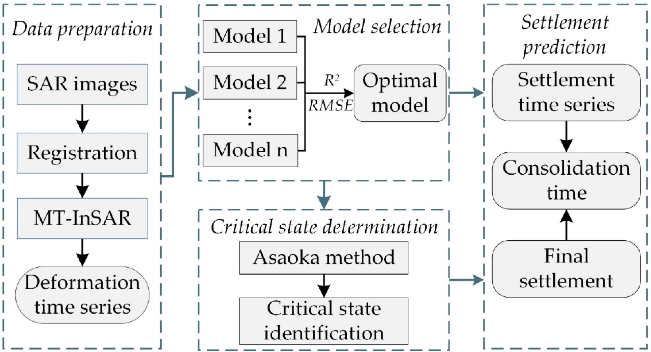
4. Methods of Settlement Prediction

The considerable number of measured points obtained from MT-InSAR provided a good opportunity for the settlement prediction of the XXIA. In this section, we discuss our methodology, according to which we chose the best model to describe the settlement pattern of the XXIA and then used the Asaoka method to estimate the termination time of settlement for predicting the total amount of settlement. The flowchart is shown in Figure 4.

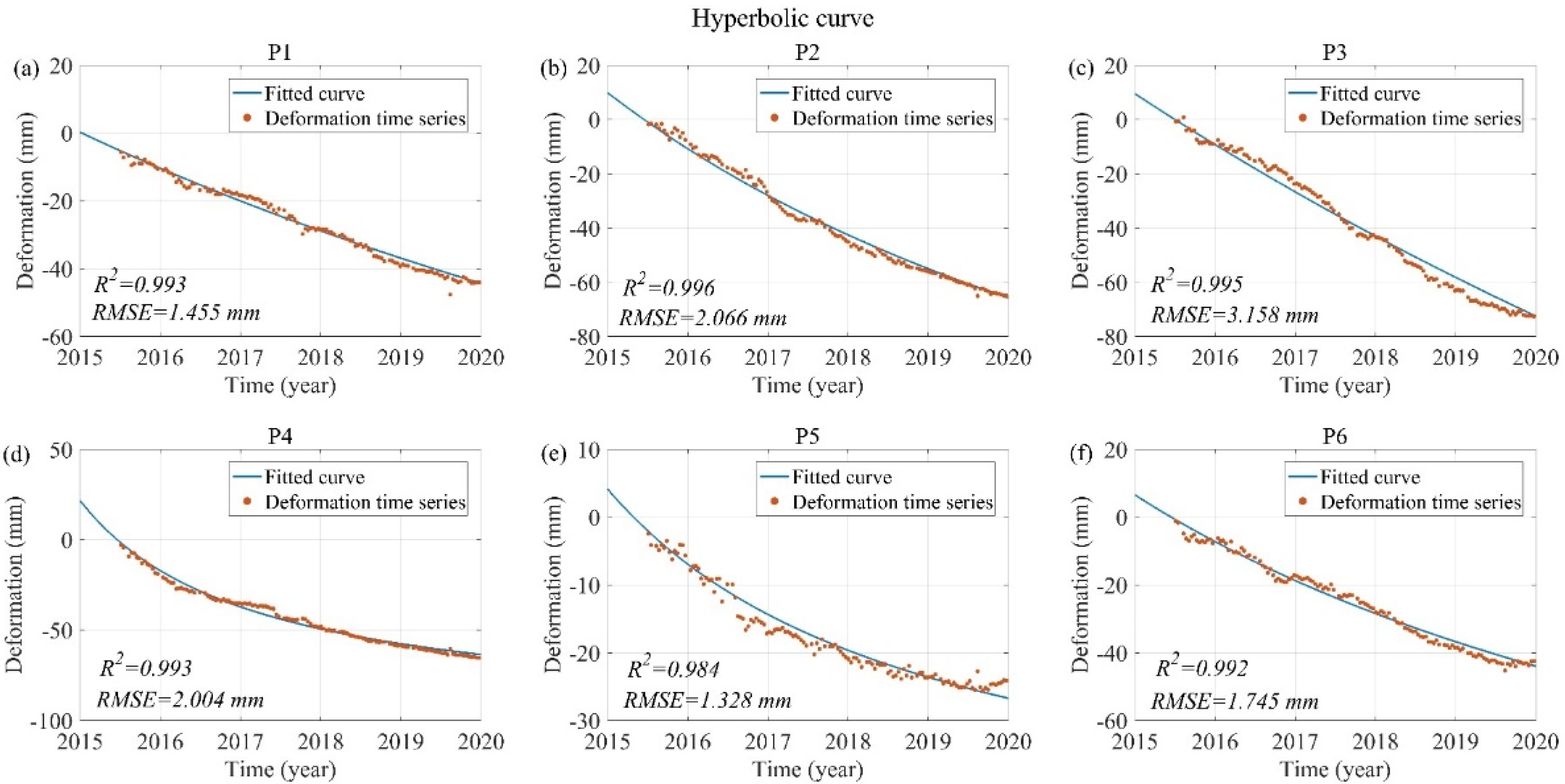
4.1. Function Model Selection

To describe the settlement patterns of the reclaimed areas, we selected the best one from three traditional curve functions—namely, the hyperbolic model, Poisson curve model, and the exponential function model—according to the deformation time series of the XXIA obtained. The three utilized models are introduced below.

4.1.1. Hyperbolic Model

The hyperbolic model [4,9,10] is an empirical curve fitting method, suitable for fitting a large amount of measured data. The amount of settlement St at time t can be expressed as
S t = S 0 + t t 0 α + β ( t t 0 )
where S0 is the initial amount of settlement, t0 is the initial time of settlement, and α and β are two unknown parameters. Formula (1) can be rewritten as
t t 0 S t S 0 = α + β ( t t 0 )
As Formula (2) shows, (tt0)/(StS0) and (tt0) are linearly related. α and β can be estimated by linear regression in t/St versus t, and then the hyperbolic model of the settlement can be determined.

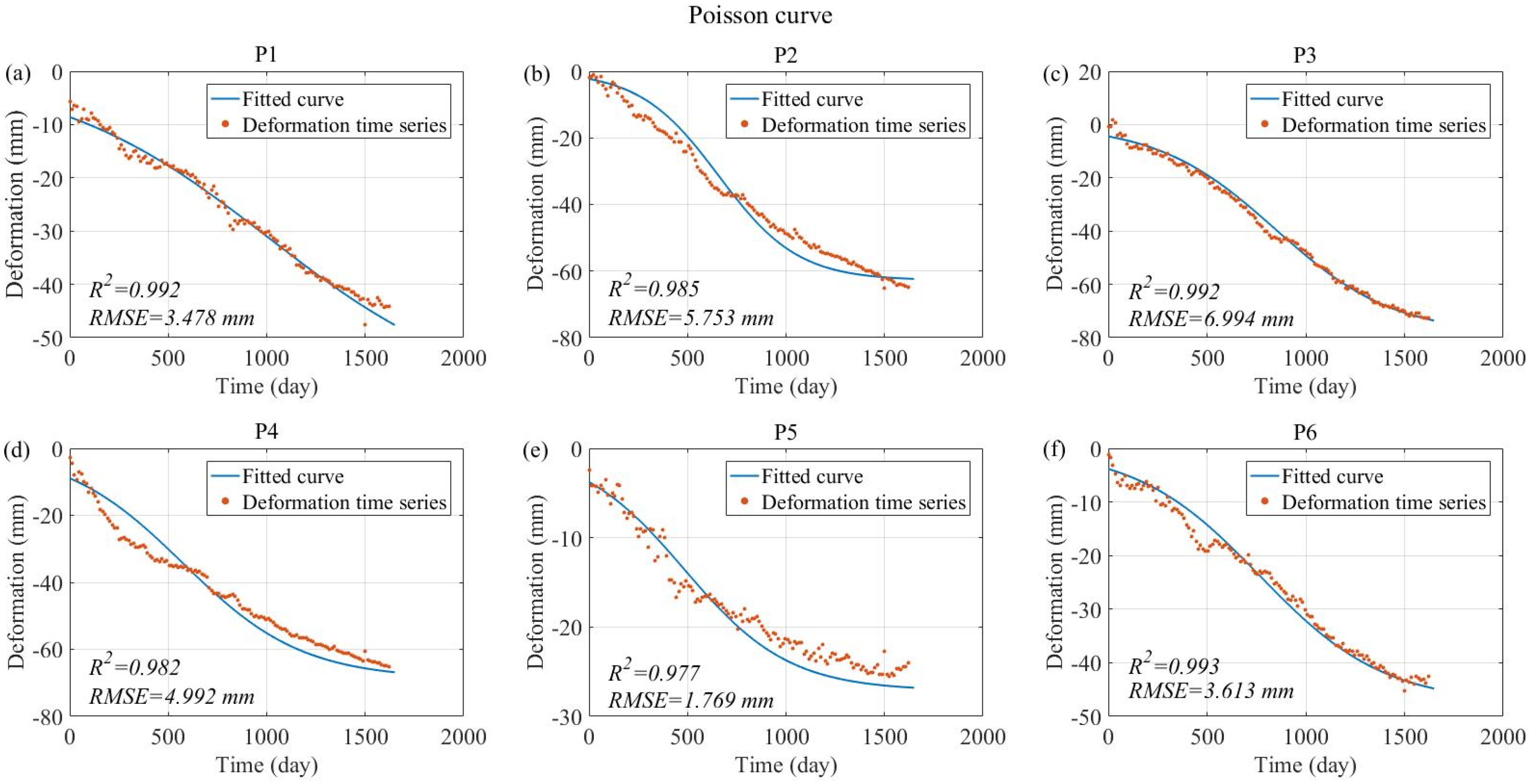
4.1.2. Poisson Curve Model

The Poisson curve model [32] can be written as
S t = c / ( 1 + a e ( b t ) )
where St represents the amount of settlement at time t. a, b, and c are three unknown parameters, which can be determined by the three-stage calculation method.
Assume the total number of SAR images is n, and the time interval of each two images is equal. The settlement time series are y1, y2, y3, …, yn. The settlement time series is divided into three groups. Each group has r = n/3 items. Let d1, d2, and d3 be the reciprocal sum of the settlement in the following three groups:
d 1 = i = 1 r 1 y i ;   d 2 = i = r + 1 2 r 1 y i ;   d 3 = i = 2 r + 1 n 1 y i
a, b, and c can be determined by the following formulas:
b = ln ( d 1 d 2 ) d 2 d 3 / r
c = r / [ d 1 ( d 1 d 2 ) 2 ( d 1 d 2 ) ( d 2 d 3 ) ]
a = ( d 1 d 2 ) 2 ( 1 e b ) c [ ( d 1 d 2 ) ( d 2 d 3 ) ] e b ( 1 e r b )
In this study, the SAR images used to retrieve the settlement time series were not acquired at equal intervals, so the settlement time series should be interpolated before applying the Poisson curve model.

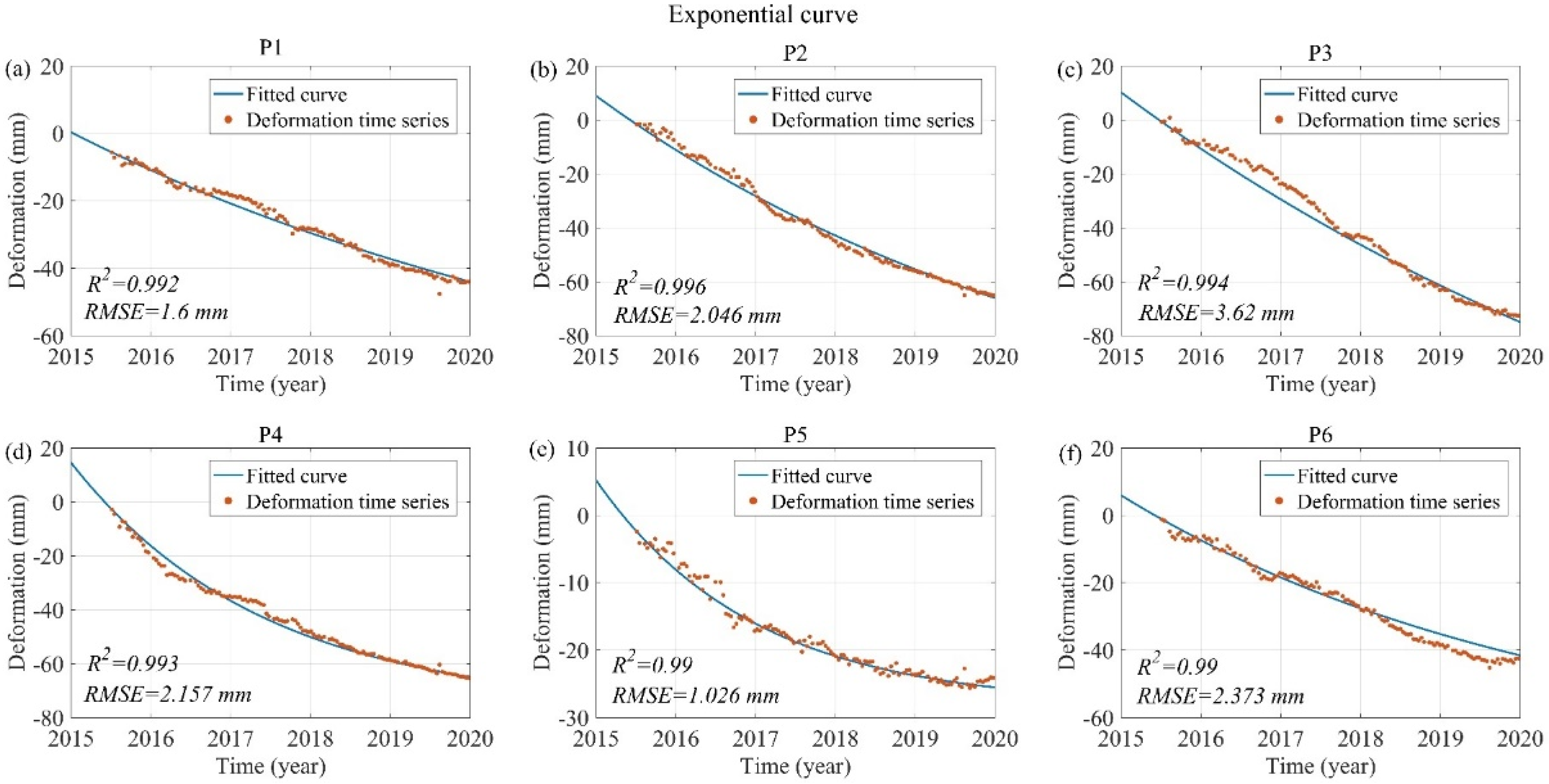
4.1.3. Exponential Function Model

The exponential function model [11,12,13] assumes that the settlement rate decreases along the exponential curve with time. The model is expressed as follows:
S t = S ( S S 0 ) e ( t 0 t ) / η
where St represents the settlement amount at time t, t0 is the initial time of settlement, η is the unknown parameter, and S0 and S represent the initial settlement amount and the final settlement amount, respectively. Nonlinear regression can be used to apply Formula (8).

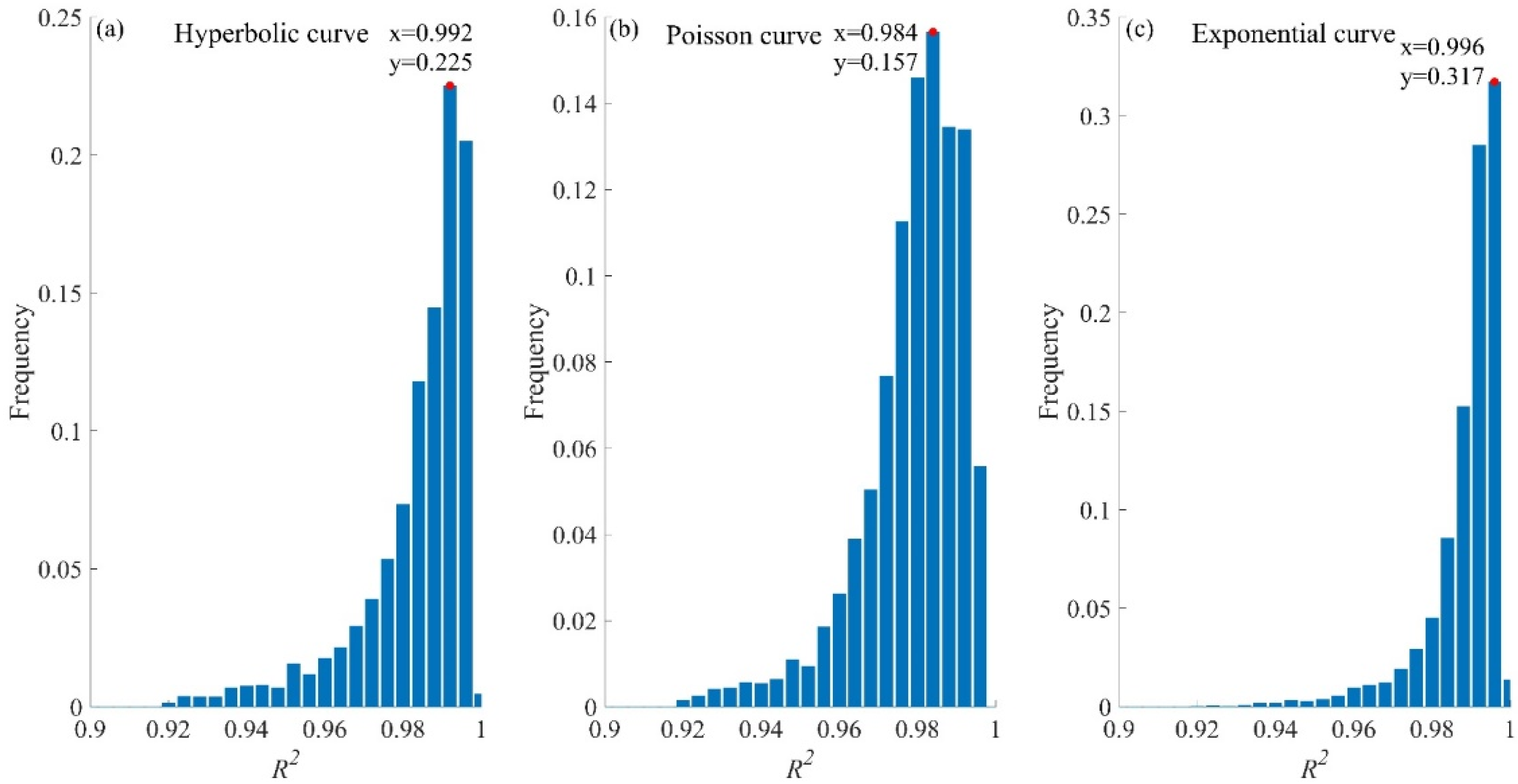
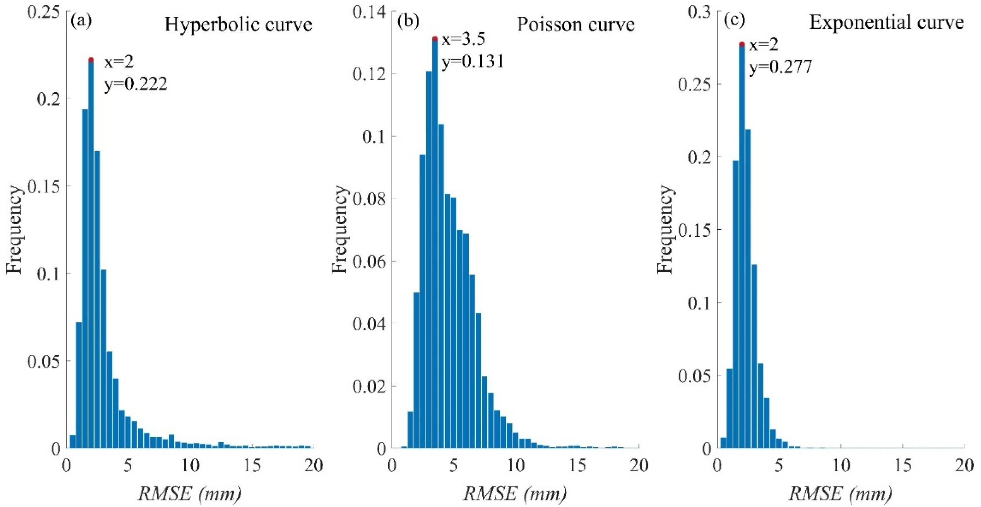
4.1.4. Optimal Model Selection

Most studies used a few points to evaluate the prediction ability of models. However, these previously selected points may not be able to describe the settlement characteristics of the whole study area. Moreover, settlement prediction based on a small number of points is not very useful in practical engineering. The optimal prediction model based on sufficient measurements can help monitor the whole study area, guide the construction process, and provide a reference for the prediction of settlement in similar cases. The application of MT-InSAR greatly contributes to the optimal model selection.
As mentioned in Section 3.2, the area reclaimed in the first phase has been subsiding for a long time. The settlement pattern can be well-represented by the long-term settlement time series of the monitored points, which helps the prediction model selection. Therefore, the settlement time series of the monitored points (4217 points) in the area reclaimed in the first phase was used to choose the optimal model from the above three models to predict the settlement. Points P1–P6 (Figure A1) were chosen to display the settlement time series and the three fitted curves (Figure 5, Figure 6 and Figure 7). As shown in Figure 5, Figure 6 and Figure 7, the three fitted curves were consistent with the settlement time series. In terms of the determination coefficient R2 and root-mean-square error (RMSE) of points P1–P6 in the curve-fitted models, the Poisson curve had the worst performance among the three models. Thus, the hyperbolic curve and exponential curve were used to predict the settlement.
We calculated the R2 and RMSE values of the 4217 monitored points to qualitatively choose the optimal curve model. Figure 8 shows the distribution of R2 of the three fitted curves. R2 of the Poisson curve was mainly concentrated around 0.984, whereas that of the hyperbolic curve was concentrated around 0.992, and the exponential curve had the highest frequency when the correlation coefficient reached 0.996. The statistical histograms of RMSE (Figure 9) showed that the maximum RMSE of the fitted exponential curves was about 7 mm, far less than that of the fitted Poisson and hyperbolic curves. The fitted exponential curves also had the minimum mean RMSE. Therefore, the exponential curve model had the best performance among the three curve models and, therefore, was determined as the optimal settlement prediction model in the study area.

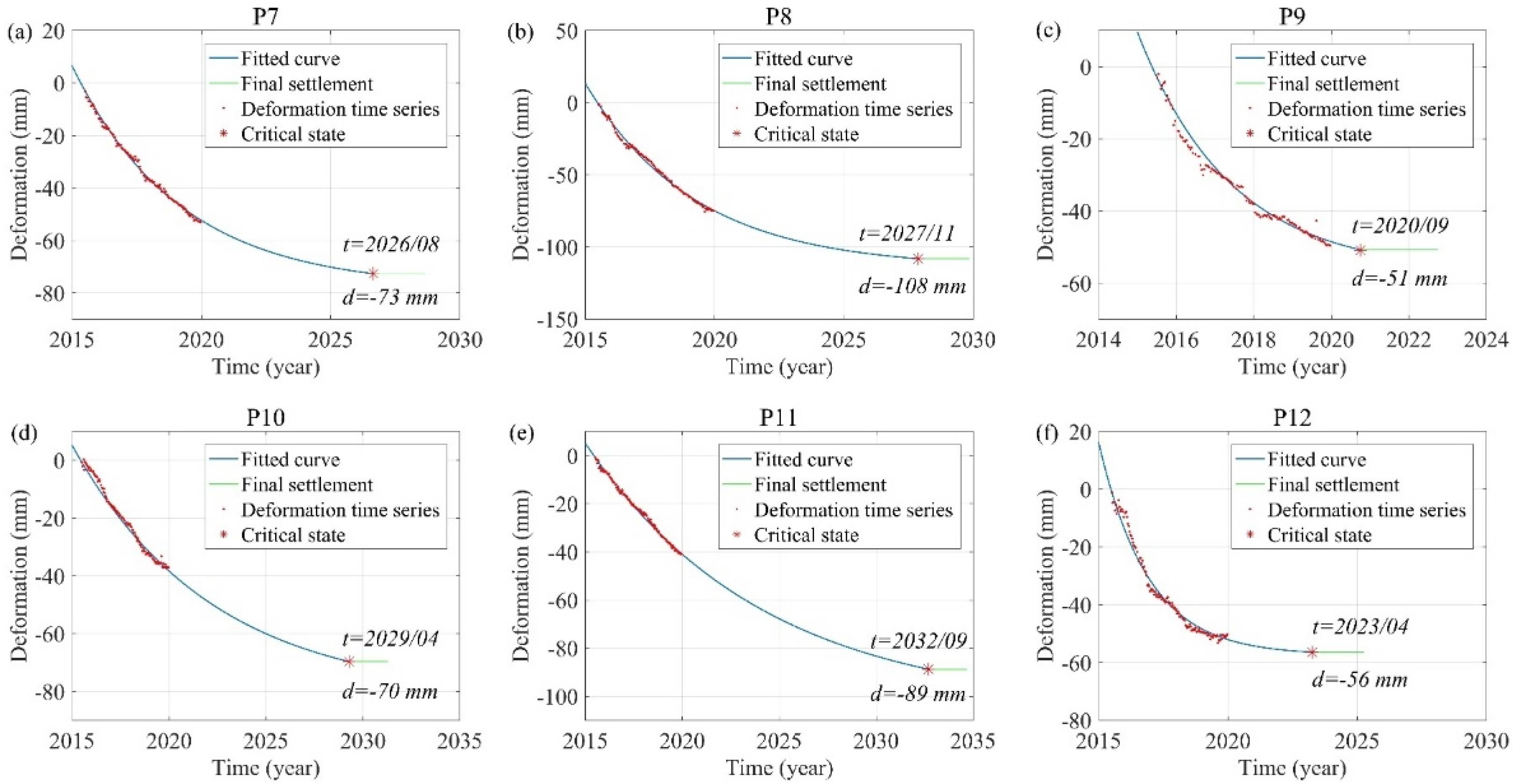
4.2. Method of Total Settlement Prediction

Although curve functions are applicable in settlement prediction, they can hardly determine when the foundation becomes stable. We used the Asaoka method [33] to identify when the settlement ends, which can obtain a reliable final settlement estimation using a large amount of measured data. Then, the total settlement was determined by combing the exponential curve model and the Asaoka method.
The Asaoka method is derived based on the Mikasa one-dimensional consolidation equation [33]. This method approximates the consolidation differential equation by the following equation:
S + λ 1 d S d t + λ 2 d 2 s d t 2 + + λ n d n s d t n = μ
where S is the total final settlement, and λ1, λ2, … λn, μ are constants.
The first-order differential of Formula (9) provides high accuracy for practical engineering applications, so Formula (9) can be rewritten as
S + λ 1 d S d t = μ
The time is divided into j (j = 1, 2, 3, …) equal parts. For time tj, the settlement is Stj, and we thus obtain
S t j + Δ t = γ 0 + γ 1 S t j
where γ0 is the settlement value, and γ1 is a constant. Linear fitting is performed on a series of scattered points ( S t j , S t j + Δ t ) to obtain the parameters γ0 and γ1, and the final settlement of the foundation is expressed as   S t = γ 0 / ( 1 γ 1 ) .

5. Discussion

5.1. Settlement Time Series Prediction

The consolidation rate of the foundation is affected by many factors, such as foundation treatment ways, the reclamation materials, and the thickness of the underlying alluvial layers, so it varies over regions [7]. It may take years or even more than ten years for some regions to reach stability under natural conditions. The prediction of the settlement time series helps locate the areas that need a long time to stabilize, so as to apply manual intervention, such as tamping and strengthening, to unstable areas and ensure that the construction is carried out on schedule. In addition, understanding the settlement behaviors can provide prior information for the planning of engineering projects.
Using the exponential curve model and the Asaoka method, we predicted the settlement time series in the XXIA. Figure 10 shows the predicted settlement curves and the settlement termination time for points P7–P12 (locations of points P7–P12 are shown in Figure A2). Their final settlement amount and the settlement termination time were different. As Figure 10 shows, under the current loads, the final settlement amount of P8 will reach about 11 cm in late 2027, and P9 will become stable within one year after December 2019. However, P7, P8, P10, and P11 need a long time for consolidation, which may be longer than ten years, exceeding the planned time of construction. Therefore, an artificial compaction process should be performed to speed up consolidation.

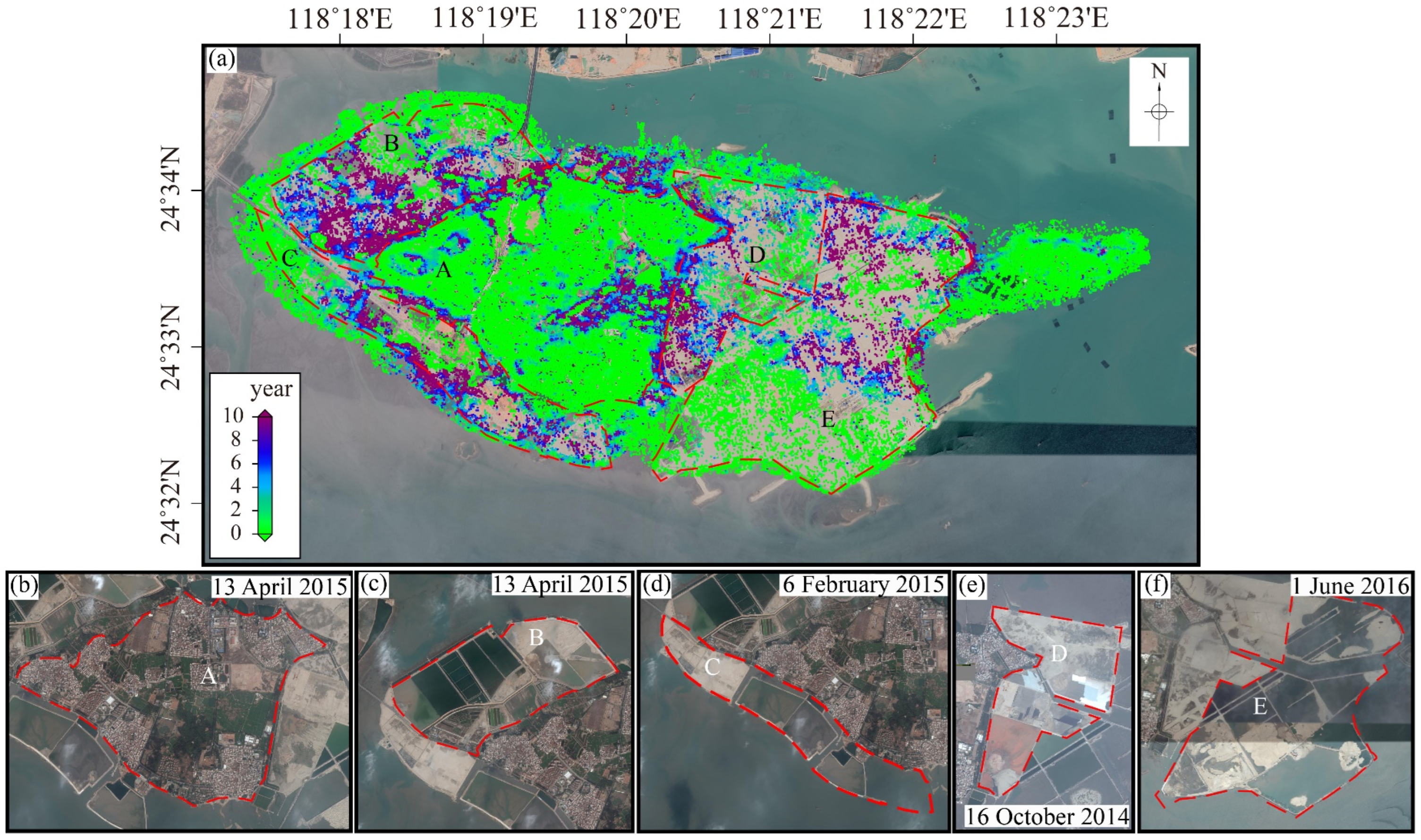
5.2. Consolidation Time Prediction of the Whole Study Area

The areas reclaimed in the first and second phases have the same geological structure and foundation treatment methods, so the settlement patterns should be similar. Therefore, we extended the optimal prediction model and the final settlement calculation method determined in Section 4 to the whole study area to analyze consolidation. We show the time required for each point to reach stabilization intuitively in Figure 11.
As Figure 11 shows, a large number of points that require more than ten years to stabilize were observed in the southern part of the area reclaimed in the first phase, the northeast part of the area reclaimed in the second phase, the northwest of Dadeng Island, and the southwest of Dadeng Island. In the interior of Dadeng Island, almost all points reached stability. Combining with the deformation rate map of the study area (Figure 3), we found that the locations of the areas with large deformation rates were coincident with that of the areas needing long settlement duration. The points with long consolidation times were mostly distributed in the reclaimed area. The type and thickness of the reclamation materials, the completion time of reclamation, and the effect of foundation treatments all affect the settlement duration. In this study, Dadeng Island and its reclamation areas were divided into five parts—namely A, B, C, D, and E. In what follows, we discuss their remaining consolidation time separately and analyze the main reasons that affect consolidation in each area.
Area A is the original land of Dadeng Island. As can be seen from Figure 11b and Figure 12, most of this area is covered by buildings, farmland, planting, and fishery farming areas, which had no changes during the InSAR monitoring period, except for a few scattered areas (Figure 3). The deformation results acquired by Liu et al. [2] and Zhuo et al. [34] also showed that there was no large-scale heavy subsidence in area A. By analyzing the optical images (Figure 12), we found that the subsidence in a few scattered areas was caused by city road construction (white dotted rectangle and Figure A3) and farmland. City road construction started between 29 April 2017 and 10 July 2017. It is reasonable that the construction activity may cause land subsidence. Therefore, the prediction results are in line with the actual condition, which further proves the reliability of the proposed method.
Area B was reclaimed in the second phase. Most of this region, except for the northeast part, needs two to ten years to consolidate. The northeast part was reclaimed before 13 April 2015, when the reclamation of the rest part of area B had not yet started (Figure 12). Therefore, when settlement in the northeast part ends, the remaining part of area B may still be in the primary consolidation stage or secondary compression stage. Similarly, areas C and E have varying consolidation times over different parts.
Area D was reclaimed in the first phase, but its northern and southern parts had different deformation rates (Figure 3). The southern part needs 4 to 10 years for consolidation. The northern part needs a shorter time to consolidate, and some parts have stopped subsiding. The first phase of the reclamation project was from March 2014 to 16 June 2015. As shown in Figure 11e, during the foundation treatment, different types of landfill materials were used in the north and south. The different landfill materials led to the different remaining settlement times.
In foundation treatment and engineering construction, special attention should be paid to the areas that need long consolidation times. However, it is worth noting that the prediction method used in this study may not be appropriate to predict the settlement in some parts of area A. Similar to the abovementioned description, farmland and some construction activity exist in area A (dry land of Dadeng Island). The subsidence patterns of farmland and some construction activity may be different from that of reclaimed areas. Therefore, the interpretation of the predicted settlement should rely on actual deformation patterns.

6. Conclusions

In this study, we focused on settlement time series, final settlement amount, and consolidation time prediction over reclaimed areas using the dense deformation measurements obtained from InSAR. The proposed method consists of two steps: (1) optimal curve model selection; (2) final settlement prediction using the Asaoka method. The Xiamen Xiang’an International Airport, a planned reclaimed area, was chosen as the study site to validate our method. A total of 128 Sentinel-1 images were used to obtain the deformation history of the study area. We analyzed the InSAR-derived deformation results and discussed the predicted settlement. The following main conclusions were drawn from this research:
(1)
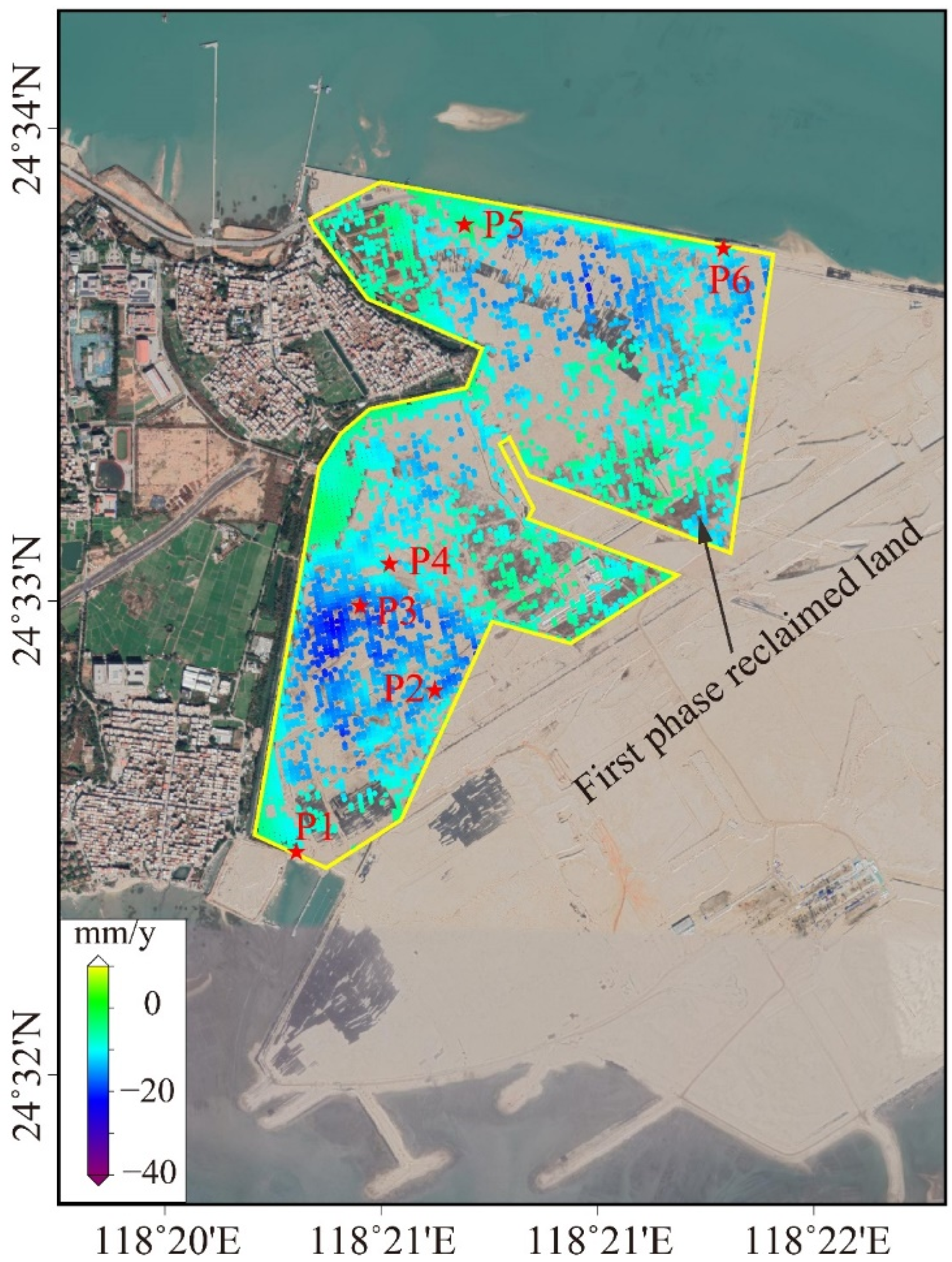
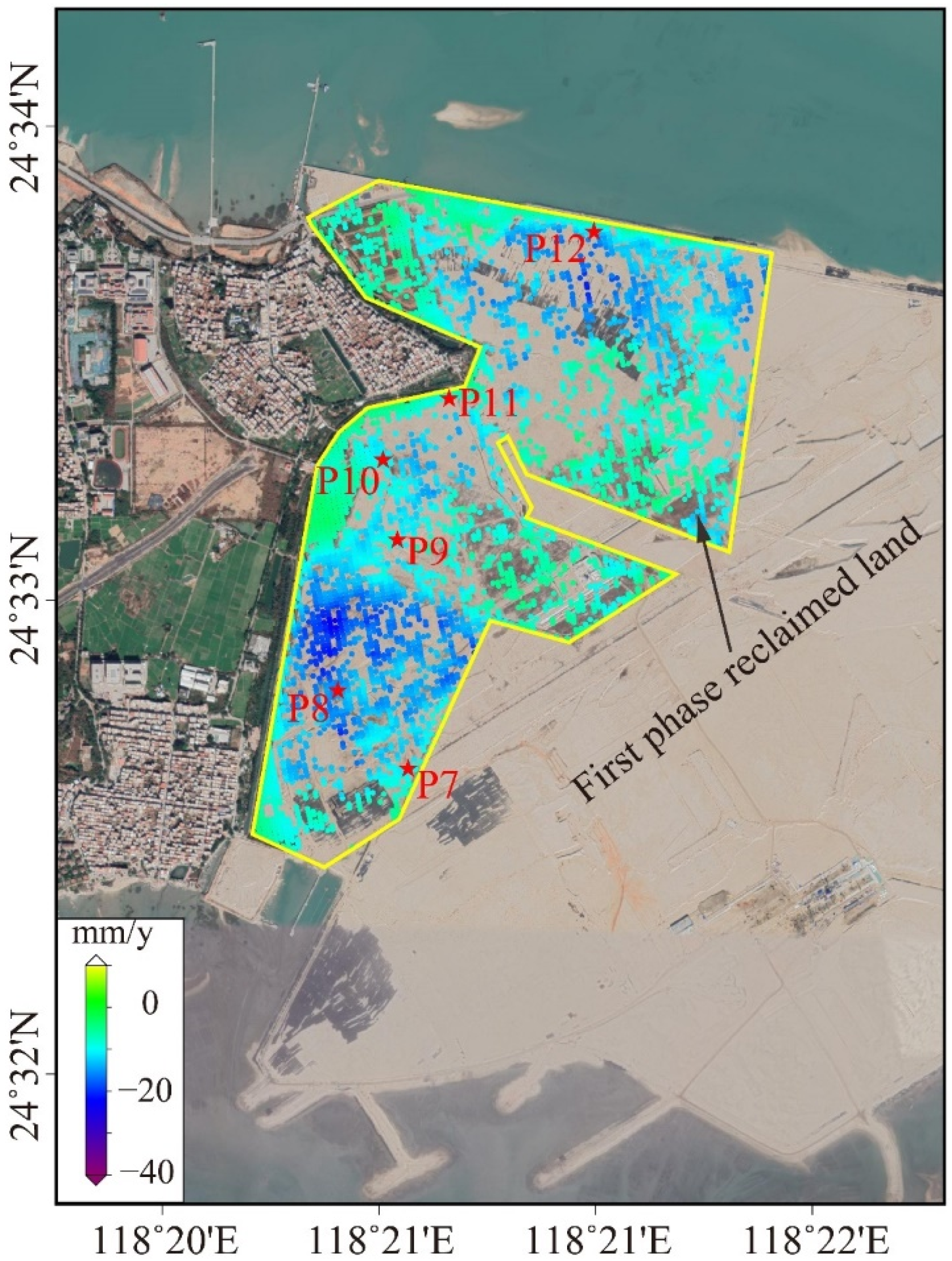
Settlement mainly occurred in the reclaimed areas, with the maximum average settlement rate exceeding 40 mm/y between 6 July 2015 and 24 December 2019. Different parts in one reclaimed area had different settlement rates, due to the uneven construction progress;
(2)
The exponential curve model showed the best performance in fitting the settlement time series obtained from MT-InSAR over the area reclaimed in the first phase. The Asaoka method was effective in the determination of deformation and stability;
(3)
The settlement time series and the final settlement of the reclaimed land could be predicted by combining the exponential curve model and the Asaoka method. Predicted consolidation time indicated that some areas need more than ten years to stabilize (since 24 December 2019). Manual consolidation should be applied to those regions to ensure construction speed.
We provided an alternative method to predict the settlement over reclaimed areas that have no in situ measurements and subsurface information. In this study, no in situ measurements or geotechnical models were used to predict the settlement, which may lead to deviation from the actual final settlement. In the future, InSAR, in situ measurements, geotechnical models, and subsurface information can be integrated to conduct precise and wide-coverage settlement predictions.

Author Contributions

Conceptualization, Z.X., K.D., G.F. and L.M.; methodology, G.F., L.M., K.L. and Y.H; writing—original draft preparation, Z.X., K.D. and L.M.; writing—review and editing, Z.X., K.D., G.F., C.H. and Y.H.; funding acquisition, G.F. All authors have read and agreed to the published version of the manuscript.

Funding

This research was supported by the National Natural Science Foundation of China (No. 42174039) and the Natural Science Foundation of Hunan Province (No. 2021JJ30807).

Data Availability Statement

The Sentinel-1 data are archived at the Copernicus Open Access Hub (https://scihub.copernicus.eu (accessed on 3 March 2020.)) and Alaska Satellite Facility (https://search.asf.alaska.edu (accessed on 6 March 2020)).

Acknowledgments

The authors would like to thank three anonymous reviewers for their constructive comments and suggestions that significantly improved this study. The authors acknowledge the GMT open-source software. The authors would like to also thank the European Space Agency (ESA) for providing the Sentinel-1 SAR images.

Conflicts of Interest

The authors declare no conflict of interest.

Appendix A

Table A1. Acquisition dates of Sentinel-1 images.
SatellitePixel Spacing (Ran × Azi)Acquisition Dates (Year/Month/Day)
Sentinel-12.3 m × 13.9 m2015/07/06, 2015/07/18, 2015/08/11, 2015/08/23, 2015/09/04, 2015/09/16, 2015/09/28, 2015/10/10, 2015/10/22, 2015/11/03, 2015/11/15, 2015/11/27,2015/12/09, 2015/12/21, 2016/01/14, 2016/01/26, 2016/02/07, 2016/02/19, 2016/03/02, 2016/03/14, 2016/03/26, 2016/04/07, 2016/04/19, 2016/05/01, 2016/05/13, 2016/05/25, 2016/06/06, 2016/06/30, 2016/07/24, 2016/08/05, 2016/08/17, 2016/08/29,2016/09/10, 2016/09/22, 2016/10/04, 2016/10/16, 2016/10/28, 2016/11/09, 2016/11/21, 2016/12/03, 2016/12/15, 2016/12/27, 2017/01/08, 2017/01/20, 2017/02/01, 2017/02/13, 2017/02/25, 2017/03/09, 2017/03/21, 2017/04/02, 2017/04/14, 2017/04/26, 2017/05/08, 2017/05/20, 2017/06/01, 2017/06/13, 2017/06/25, 2017/07/19, 2017/07/31, 2017/08/12,
2017/08/24, 2017/09/05, 2017/09/17, 2017/10/11, 2017/10/23, 2017/11/04, 2017/11/16, 2017/11/28, 2017/12/10, 2017/12/22, 2018/01/03, 2018/01/15, 2018/01/27, 2018/02/08, 2018/02/20, 2018/03/04, 2018/03/28, 2018/04/09, 2018/04/21, 2018/05/03, 2018/05/15, 2018/05/27, 2018/06/08, 2018/06/20, 2018/07/02, 2018/07/14, 2018/07/26, 2018/08/07, 2018/08/19, 2018/08/31, 2018/09/12, 2018/09/24, 2018/10/06, 2018/10/18, 2018/11/11, 2018/11/23, 2018/12/05, 2018/12/17, 2018/12/29, 2019/01/10, 2019/01/22, 2019/02/03, 2019/02/27, 2019/03/11, 2019/03/23, 2019/04/04, 2019/04/16, 2019/04/28, 2019/05/10, 2019/05/22, 2019/06/03, 2019/06/15, 2019/06/27, 2019/07/09, 2019/07/21, 2019/08/02, 2019/08/14, 2019/08/26, 2019/09/07, 2019/09/19, 2019/10/01, 2019/10/13, 2019/10/25, 2019/11/06, 2019/11/18, 2019/11/30, 2019/12/12, 2019/12/24
Figure A1. Locations of points P1–P6.
Remotesensing 14 03081 g0a1
Figure A2. Locations of points P7–P12.
Remotesensing 14 03081 g0a2
Figure A3. Optical images of the white dotted rectangle area in Figure 12. Optical image acquired on (a) 16 June 2015, (b) 24 June 2016, (c) 10 July 2017, (d) 2 June 2018, (e) 26 July 2019, and (f) 7 December 2019.
Remotesensing 14 03081 g0a3

References

  1. Yu, Q.; Yan, X.; Wang, Q.; Yang, T.; Lu, W.; Yao, M.; Dong, J.; Zhan, J.; Huang, X.; Niu, C.; et al. A Spatial-Scale Evaluation of Soil Consolidation Concerning Land Subsidence and Integrated Mechanism Analysis at Macro-, and Micro-Scale: A Case Study in Chongming East Shoal Reclamation Area, Shanghai, China. Remote Sens. 2021, 13, 2418. [Google Scholar] [CrossRef]
  2. Liu, X.; Zhao, C.; Zhang, Q.; Yang, C.; Zhang, J. Characterizing and Monitoring Ground Settlement of Marine Reclamation Land of Xiamen New Airport, China with Sentinel-1 SAR Datasets. Remote Sens. 2019, 11, 585. [Google Scholar] [CrossRef] [Green Version]
  3. Wang, W.; Liu, H.; Li, Y.; Su, J. Development and management of land reclamation in China. Ocean Coastal Manag. 2014, 102, 415–425. [Google Scholar] [CrossRef]
  4. Park, S.; Hong, S. Nonlinear Modeling of Subsidence from a Decade of InSAR Time Series. Geophys. Res. Lett. 2021, 48, 2020GL090970. [Google Scholar] [CrossRef]
  5. Pepe, A.; Bonano, M.; Zhao, Q.; Yang, T.; Wang, H. The Use of C-/X-Band Time-Gapped SAR Data and Geotechnical Models for the Study of Shanghai’s Ocean-Reclaimed Lands through the SBAS-DInSAR Technique. Remote Sens. 2016, 8, 911. [Google Scholar] [CrossRef] [Green Version]
  6. Nadeem, M.; Akbar, M.; Pan, H.; Li, X.; Ou, G.; Amin, A. Investigation of the settlement prediction in soft soil by Richards Model: Based on a linear least squares-iteration method. Arch. Civ. Eng. 2021, 67, 491–506. [Google Scholar] [CrossRef]
  7. Jiang, L.; Lin, H. Integrated analysis of SAR interferometric and geological data for investigating long-term reclamation settlement of Chek Lap Kok Airport, Hong Kong. Eng. Geol. 2010, 110, 77–92. [Google Scholar] [CrossRef]
  8. Mei, G.; Zhao, X.; Wang, Z. Settlement Prediction Under Linearly Loading Condition. Mar. Geores. Geotechnol. 2015, 33, 92–97. [Google Scholar] [CrossRef]
  9. Kim, S.; Wdowinski, S.; Dixon, T.; Amelung, F.; Kim, J.; Won, J. Measurements and predictions of subsidence induced by soil consolidation using persistent scatterer InSAR and a hyperbolic model. Geophys. Res. Lett. 2010, 37. [Google Scholar] [CrossRef] [Green Version]
  10. Al-Shamrani, M. Applying the hyperbolic method and C-alpha/C-c concept for settlement prediction of complex organic-rich soil formations. Eng. Geol. 2005, 77, 17–34. [Google Scholar] [CrossRef]
  11. Hu, X.; Liang, X.; Yu, Y.; Guo, S.; Cui, Y.; Li, Y.; Qi, S. Remote Sensing Characterization of Mountain Excavation and City Construction in Loess Plateau. Geophys. Res. Lett. 2021, 48. [Google Scholar] [CrossRef]
  12. Chaussard, E.; Bürgmann, R.; Shizaei, M.; Fielding, E.; Baker, B. Predictability of hydraulic head changes and characterization of aquifer-system and fault properties from InSAR-derived ground deformation. J. Geophys. Res.-Solid Earth 2014, 119, 6572–6590. [Google Scholar] [CrossRef]
  13. Shi, G.; Ma, P.; Hu, X.; Huang, B.; Lin, H. Surface response and subsurface features during the restriction of groundwater exploitation in Suzhou (China) inferred from decadal SAR interferometry. Remote Sens. Environ. 2021, 256, 112327. [Google Scholar] [CrossRef]
  14. Ren, X.; Tang, Y.; Li, J.; Yang, Q. A prediction method using grey model for cumulative plastic deformation under cyclic loads. Nat. Hazards 2012, 64, 441–457. [Google Scholar] [CrossRef]
  15. Deng, Z.; Ke, Y.; Gong, H.; Li, X.; Li, Z. Land subsidence prediction in Beijing based on PS-InSAR technique and improved Grey-Markov model. GISci. Remote Sens. 2017, 54, 797–818. [Google Scholar] [CrossRef]
  16. Chen, P.; Yu, H. Foundation Settlement Prediction Based on a Novel NGM Model. Math. Probl. Eng. 2014, 2014, 242809. [Google Scholar] [CrossRef]
  17. Shi, G.; Lin, H.; Bürgmann, R.; Ma, P.; Wang, J.; Liu, Y. Early soil consolidation from magnetic extensometers and full resolution SAR interferometry over highly decorrelated reclaimed lands. Remote Sens. Environ. 2019, 231, 111231. [Google Scholar] [CrossRef]
  18. Xiong, Z.; Feng, G.; Feng, Z.; Miao, L.; Wang, Y.; Yang, D. Pre- and post-failure spatial-temporal deformation pattern of the Baige landslide retrieved from multiple radar and optical satellite images. Eng. Geol. 2020, 279, 105880. [Google Scholar] [CrossRef]
  19. Hu, X.; Bürgmann, R.; Schulz, W.; Fielding, E. Four-dimensional surface motions of the Slumgullion landslide and quantification of hydrometeorological forcing. Nat. Commun. 2020, 11, 2792. [Google Scholar] [CrossRef]
  20. Xu, Q.; Guo, C.; Dong, X.; Li, W.; Lu, H.; Fu, H.; Liu, X. Mapping and Characterizing Displacements of Landslides with InSAR and Airborne LiDAR Technologies: A Case Study of Danba County, South west China. Remote Sens. 2021, 13, 4234. [Google Scholar] [CrossRef]
  21. He, L.; Feng, G.; Wu, X.; Lu, H.; Xu, W.; Wang, Y.; Liu, J.; Hu, J.; Li, Z. Coseismic and Early Postseismic Slip Models of the 2021 Mw7.4 Maduo Earthquake (Western China) Estimated by Space-Based Geodetic Data. Geophys. Res. Lett. 2021, 48. [Google Scholar] [CrossRef]
  22. Zhou, Y.; Thomas, M.; Parsons, B.; Walker, R. Time-dependent postseismic slip following the 1978 Mw 7.3 Tabas-e-Golshan, Iran earthquake revealed by over 20 years of ESA InSAR observations. Earth Planet. Sci. Lett. 2018, 483, 64–75. [Google Scholar] [CrossRef]
  23. Huang, M.; Fielding, E.; Liang, G.; Milillo, P.; Bekaert, D.; Dreger, D.; Salzer, J. Coseismic deformation and triggered landslides of the 2016 Mw 6.2 Amatrice earthquake in Italy. Geophys. Res. Lett. 2017, 44, 1266–1274. [Google Scholar] [CrossRef] [Green Version]
  24. Xu, W.; Xie, L.; Aoki, Y.; Rivalta, E.; Jónsson, S. Volcano-Wide Deformation After the 2017 Erta Ale Dike Intrusion, Ethiopia, Observed with Radar Interferometry. J. Geophys. Res.-Solid Earth 2020, 125. [Google Scholar] [CrossRef]
  25. Hooper, A.; Zebker, H.; Segall, P.; Kampes, B. A new method for measuring deformation on volcanoes and other natural terrains using InSAR persistent scatterers. Geophys. Res. Lett. 2004, 31. [Google Scholar] [CrossRef]
  26. Peng, M.; Lu, Z.; Zhao, C.; Motagh, M.; Bai, L.; Conway, B.; Chen, H. Mapping land subsidence and aquifer system properties of the Willcox Basin, Arizona, from InSAR observations and independent component analysis. Remote Sens. Environ. 2022, 271, 112894. [Google Scholar] [CrossRef]
  27. Xu, B.; Feng, G.; Li, Z.; Wang, Q.; Wang, C.; Xie, R. Coastal Subsidence Monitoring Associated with Land Reclamation Using the Point Target Based SBAS-InSAR Method: A Case Study of Shenzhen, China. Remote Sens. 2016, 8, 652. [Google Scholar] [CrossRef] [Green Version]
  28. Costantini, M.; Ferretti, A.; Minati, F.; Falco, S.; Trillo, F.; Colombo, D.; Novali, F.; Malvarosa, F.; Mammone, C.; Vecchioli, F.; et al. Analysis of surface deformation over the whole Italian territory by interferometric processing of ERS, Envisat and COSMO-SkyMed radar data. Remote Sens. Environ. 2017, 202, 250–275. [Google Scholar] [CrossRef]
  29. Ma, P.; Wang, W.; Zhang, B.; Wang, J.; Shi, G.; Huang, G.; Chen, F.; Jiang, L.; Lin, H. Remotely sensing large- and small-scale ground subsidence: A case study of the Guangdong-Hong Kong-Macao Greater Bay Area of China. Remote Sens. Environ. 2019, 232, 111282. [Google Scholar] [CrossRef]
  30. Wang, Y.; Feng, G.; Li, Z.; Xu, W.; Zhu, J.; He, L.; Xiong, Z.; Qiao, X. Retrieving the displacements of the Hutubi (China) underground gas storage during 2003–2020 from multi-track InSAR. Remote Sens. Environ. 2022, 268, 112768. [Google Scholar] [CrossRef]
  31. Yang, C.; Zhang, D.; Zhao, C.; Han, B.; Sun, R.; Du, J.; Chen, L. Ground Deformation Revealed by Sentinel-1 MSBAS-InSAR Time-Series over Karamay Oilfield, China. Remote Sens. 2019, 11, 2027. [Google Scholar] [CrossRef] [Green Version]
  32. Zhu, L.; Xing, X.; Zhu, Y.; Peng, W.; Yuan, Z.; Xia, Q. An Advanced Time-Series InSAR Approach Based on Poisson Curve for Soft Clay Highway Deformation Monioring. IEEE J.-STARS 2021, 14, 7682–7698. [Google Scholar] [CrossRef]
  33. Asaoka, A. Observational Procedure of Settlement Prediction. Soils Found. 1978, 18, 87–101. [Google Scholar] [CrossRef] [Green Version]
  34. Zhuo, G.; Dai, K.; Huang, H.; Li, S.; Shi, X.; Feng, Y.; Li, T.; Dong, X.; Deng, J. Evaluating Potential Ground Subsidence Geo-Hazard of Xiamen Xiang’an New Airport on Reclaimed Land by SAR Interferometry. Sustainability 2020, 12, 6991. [Google Scholar] [CrossRef]
  35. Ferretti, A.; Prati, C.; Rocca, F. Permanent scatterers in SAR interferometry. IEEE Trans. Geosci. Remote Sens. 2001, 39, 8–20. [Google Scholar] [CrossRef]
  36. Berardino, P.; Fornaro, G.; Lanari, R.; Sansosti, E. A new algorithm for surface deformation monitoring based on small baseline differential SAR interferograms. IEEE Trans. Geosci. Remote Sens. 2002, 40, 2375–2383. [Google Scholar] [CrossRef] [Green Version]
Figure 1. The Xiamen Xiang’an International Airport (XXIA): (a) coverage of Sentinel-1 images and the location of the XXIA; (b) optical image of Dadeng Island; (c) location of the XXIA in Fujian Province, China.
Remotesensing 14 03081 g001
Figure 2. Optical images of the XXIA, Dadeng Island, and Xiaodeng Island: (a) illustration of the three phases of land reclamation. The yellow, white, and red lines are the boundaries of the reclaimed land in the first, second, and third phases, respectively. The blue line represents the dry land of Dadeng Island; (bd) optical images of the study area acquired in December 2011, December 2015, and December 2019, respectively. The green lines delineate the boundaries of Dadeng Island and Xiaodeng Island.
Remotesensing 14 03081 g002
Figure 3. Average deformation rate map of the study area. Positive values denote the deformation toward the satellite. Negative values denote the deformation away from the satellite: (a) average deformation rate map of the whole study area; (be) enlarged view of areas outlined by dotted lines in (a).
Remotesensing 14 03081 g003
Figure 4. Flowchart of the settlement prediction.
Remotesensing 14 03081 g004
Figure 5. Hyperbolic curve fitting of (a) P1, (b) P2, (c) P3, (d) P4, (e) P5 and (f) P6. Locations of points P1−P6 are shown in Figure A1.
Remotesensing 14 03081 g005
Figure 6. Poisson curve fitting of (a) P1, (b) P2, (c) P3, (d) P4, (e) P5 and (f) P6. Locations of points P1−P6 are shown in Figure A1.
Remotesensing 14 03081 g006
Figure 7. Exponential curve fitting of (a) P1, (b) P2, (c) P3, (d) P4, (e) P5 and (f) P6. Locations of points P1−P6 are shown in Figure A1.
Remotesensing 14 03081 g007
Figure 8. R2 of (a) Hyperbolic curve fitting, (b) Poisson curve fitting and (c) Exponential curve fitting.
Remotesensing 14 03081 g008
Figure 9. RMSE of (a) Hyperbolic curve fitting, (b) Poisson curve fitting and (c) Exponential curve fitting.
Remotesensing 14 03081 g009
Figure 10. Predicted settlement curves of (a) P7, (b) P8, (c) P9, (d) P10, (e) P11 and (f) P12. Locations of points P7−P12 are shown in Figure A2. t is the consolidation time, and d is the final settlement.
Remotesensing 14 03081 g010
Figure 11. (a) The time needed for stabilization since the acquisition date (24 December 2019) of Dadeng Island and its reclamation areas: (b) optical image of area A acquired on 13 April 2015; (c) optical image of area B acquired on 13 April 2015; (d) optical image of area C acquired on 6 February 2015; (e) optical image of area D acquired on 16 October 2014; (f) optical image of area E acquired on 1 June 2016.
Remotesensing 14 03081 g011
Figure 12. Optical images of the study area acquired on (a) 16 June 2015, (b) 24 June 2016, (c) 29 April 2017, (d) 10 July 2017, (e) 2 June 2018, (f) 26 July 2019, and (g) 7 December 2019.
Remotesensing 14 03081 g012
Table 1. Acquisition dates and parameters of the collected Sentinel-1 images.
SensorsDirectionIncidence AnglePath-FrameNumber of ImagesTemporal
Coverage
Sentinel-1Ascending33.91°142-751286 July 2015–24 December 2019
Publisher’s Note: MDPI stays neutral with regard to jurisdictional claims in published maps and institutional affiliations.

