
STF-EGFA: A Remote Sensing Spatiotemporal Fusion Network with Edge-Guided Feature Attention


Abstract
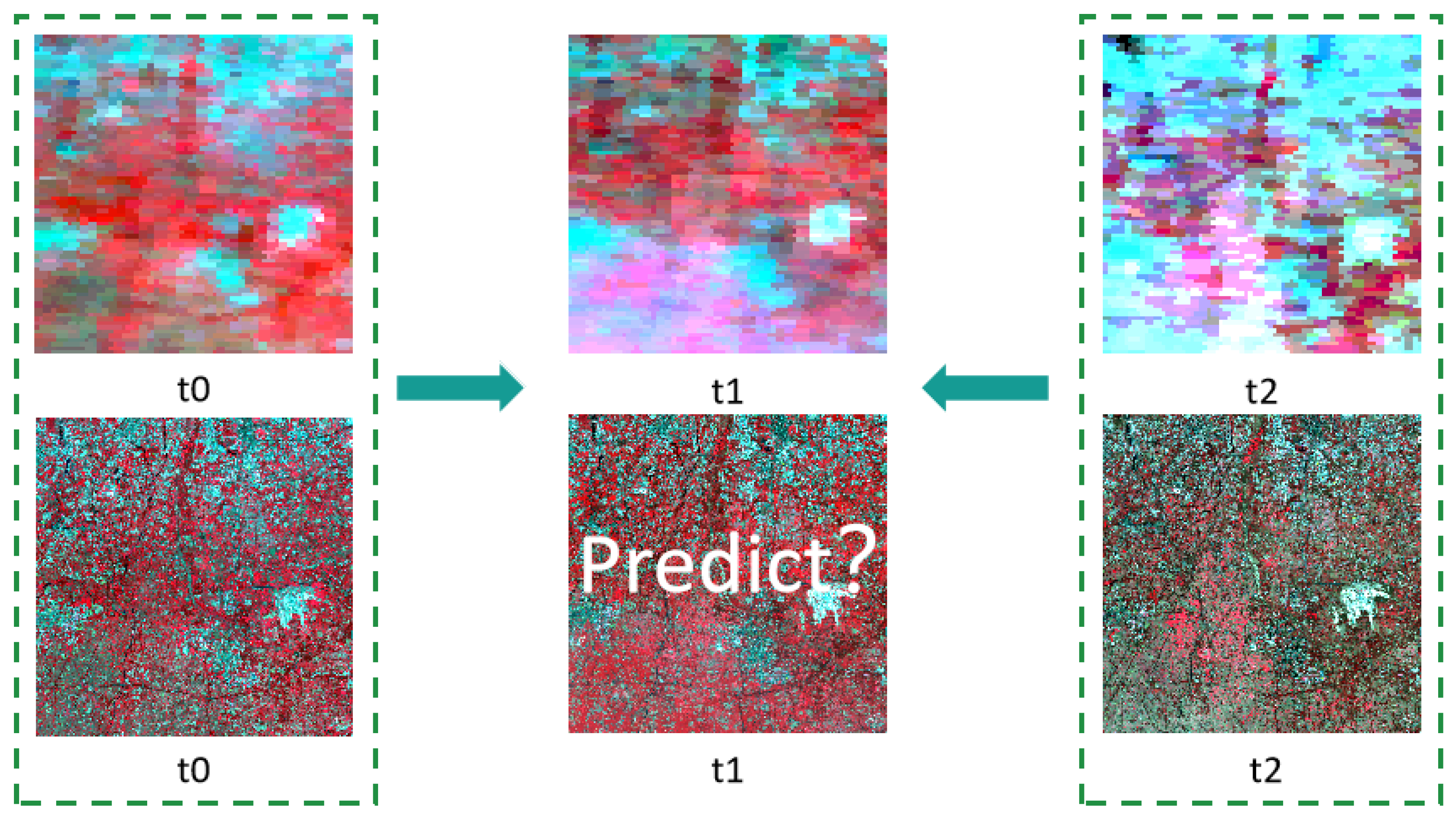
:1. Introduction
2. Related Work
- We design a spatiotemporal fusion method with edge-guided feature attention based on remote sensing, called STF-EGFA, which strengthens the connections among features in different layers and reduces information loss while utilizing multilayer features.
- The edge extraction module in STF-EGFA is mainly designed to decrease the boundary information loss in the process of feature extraction and improve the retention of edge details at high spatial resolution to ensure that the predicted spatiotemporal images retain more saliency.
- The design of the feature attention (FA) module in STF-EGFA focuses on the key available information by using an FA mechanism guided by edge information. Information weighting and pixel heterogeneity are optimized among different channels in the network to provide more accurate predictions of spatiotemporal changes.
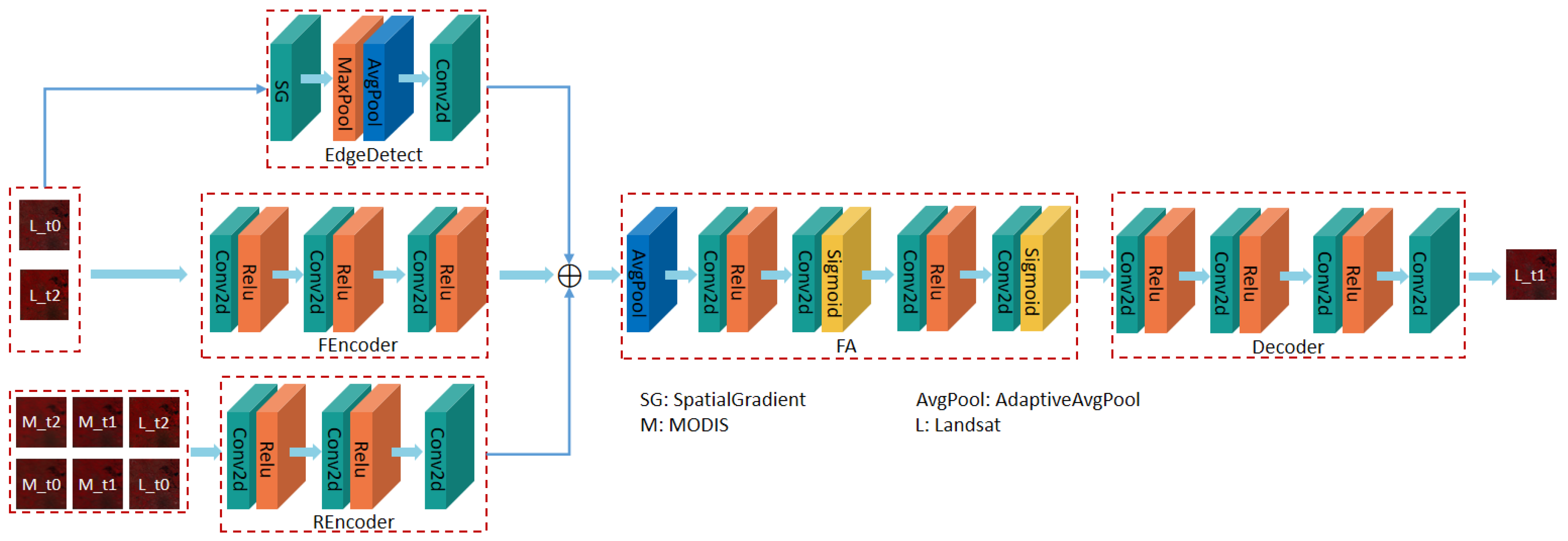
3. Methods
3.1. Edge Feature Extraction
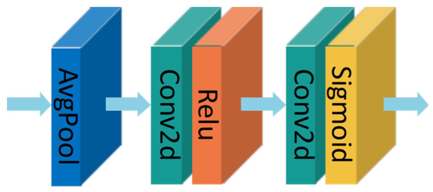
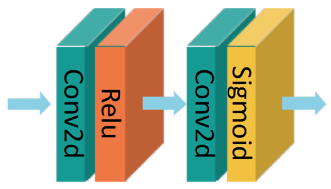
3.2. Feature Attention
3.2.1. Channel Attention
3.2.2. Pixel Attention
3.3. Loss Function
4. Experiments and Evaluations
4.1. Datasets
4.1.1. AHB Dataset
4.1.2. Tianjin Dataset
4.1.3. Daxing Dataset
4.2. Evaluation
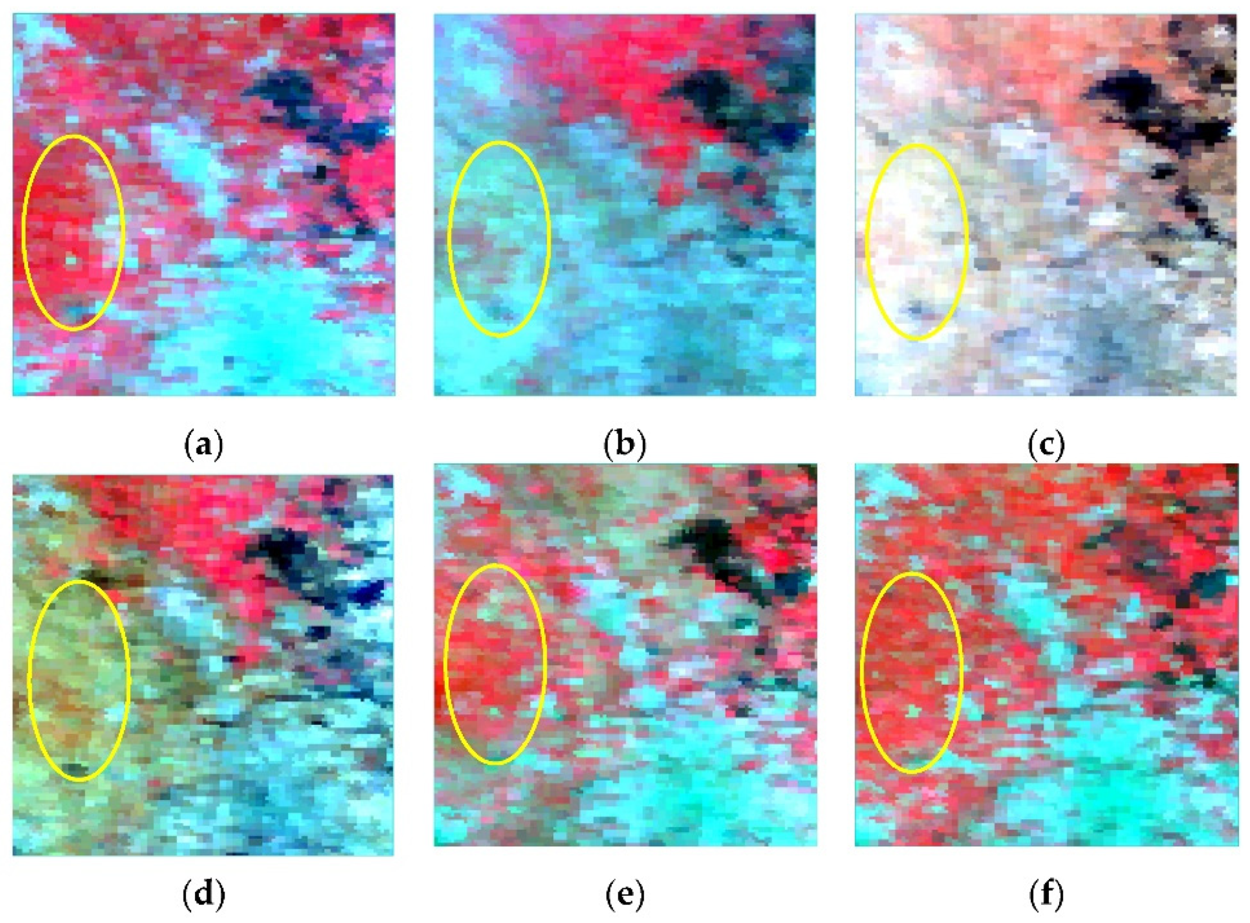
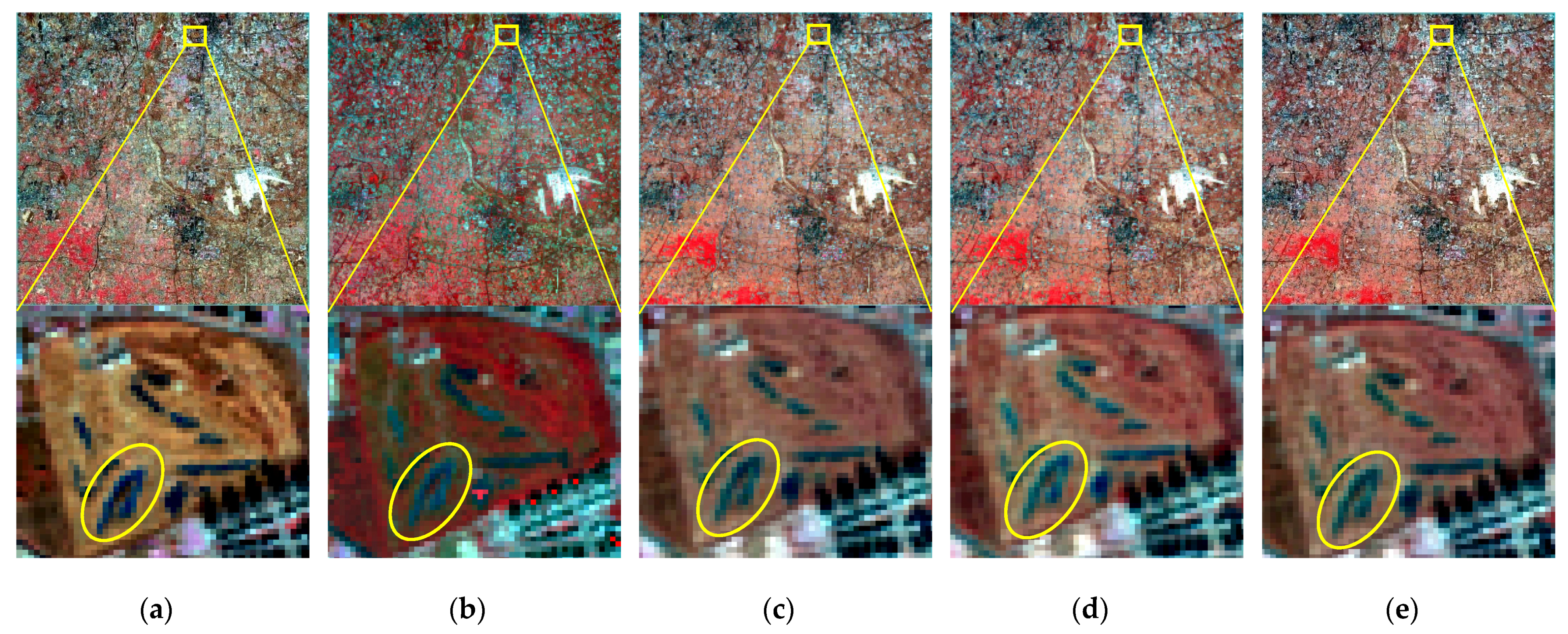
4.3. Experimental Results and Analysis
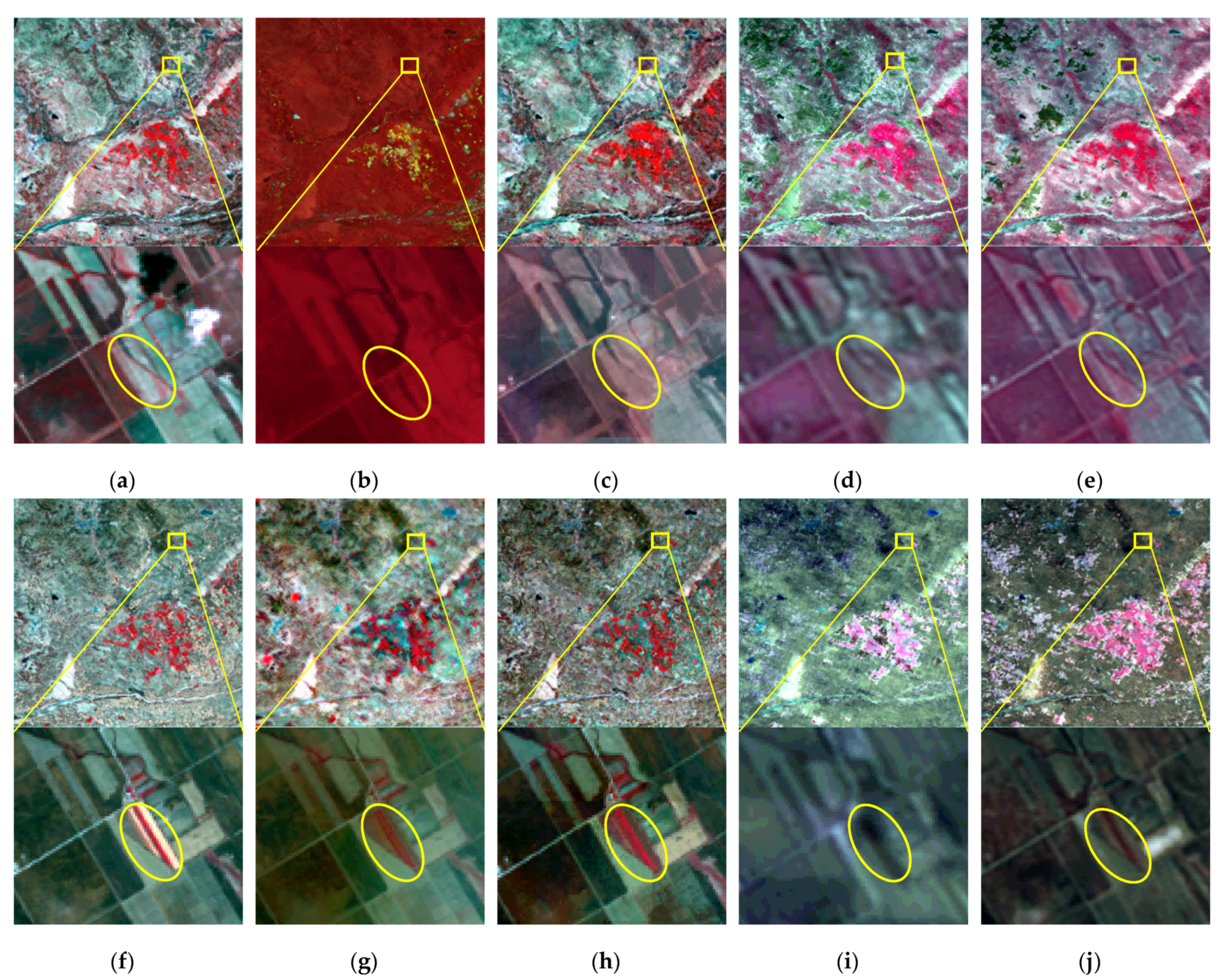
4.3.1. AHB Dataset
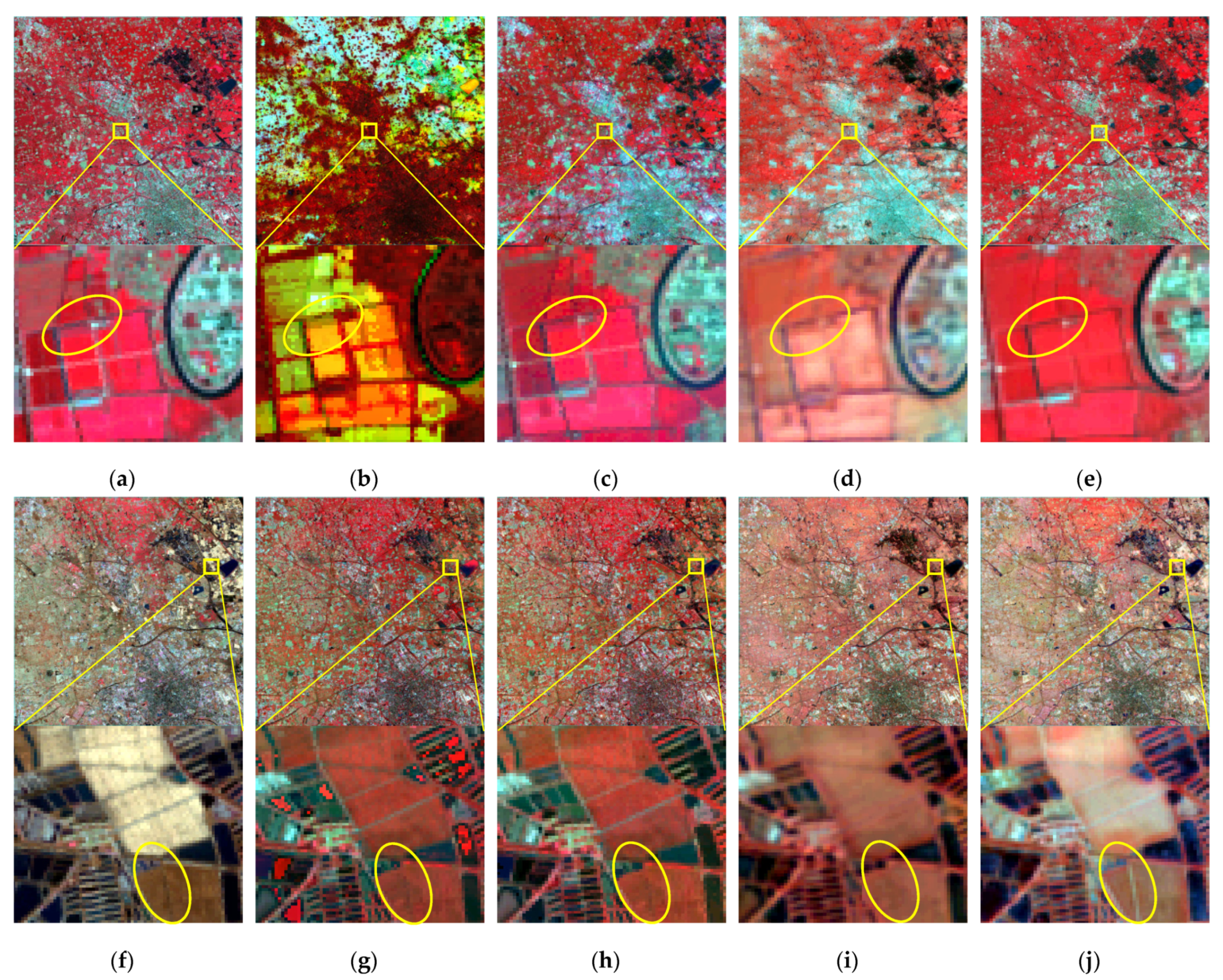
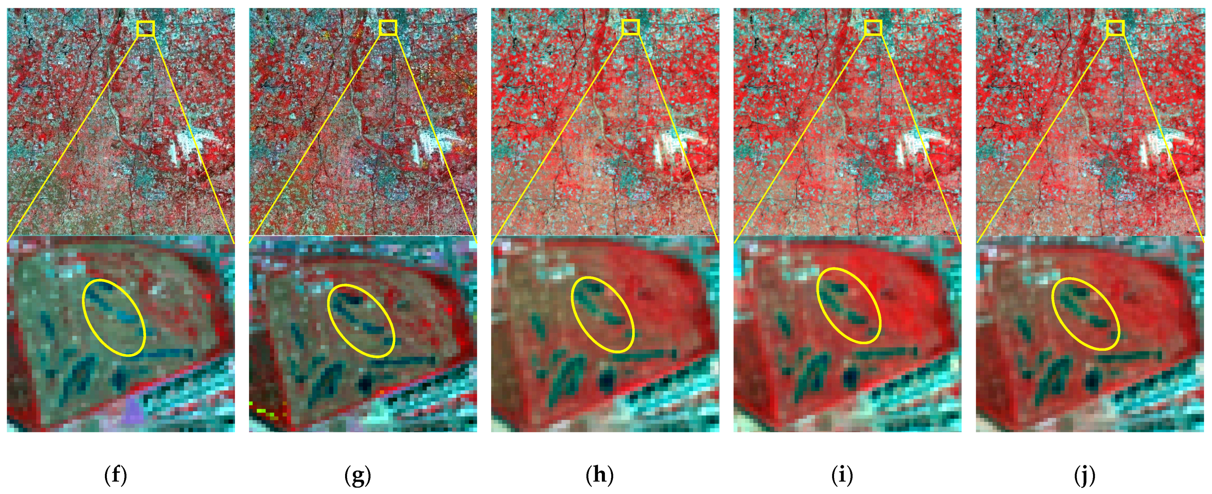
4.3.2. Tianjin Dataset
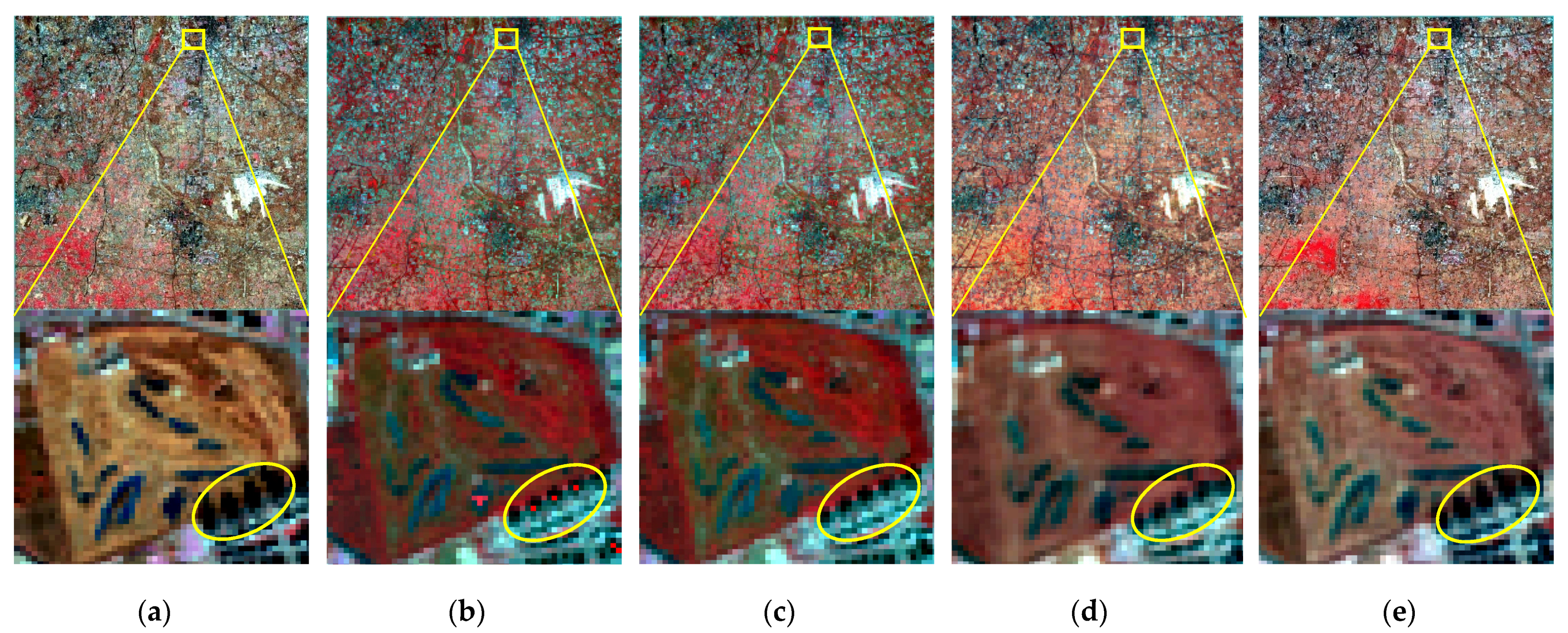
4.3.3. Daxing Dataset
5. Discussion
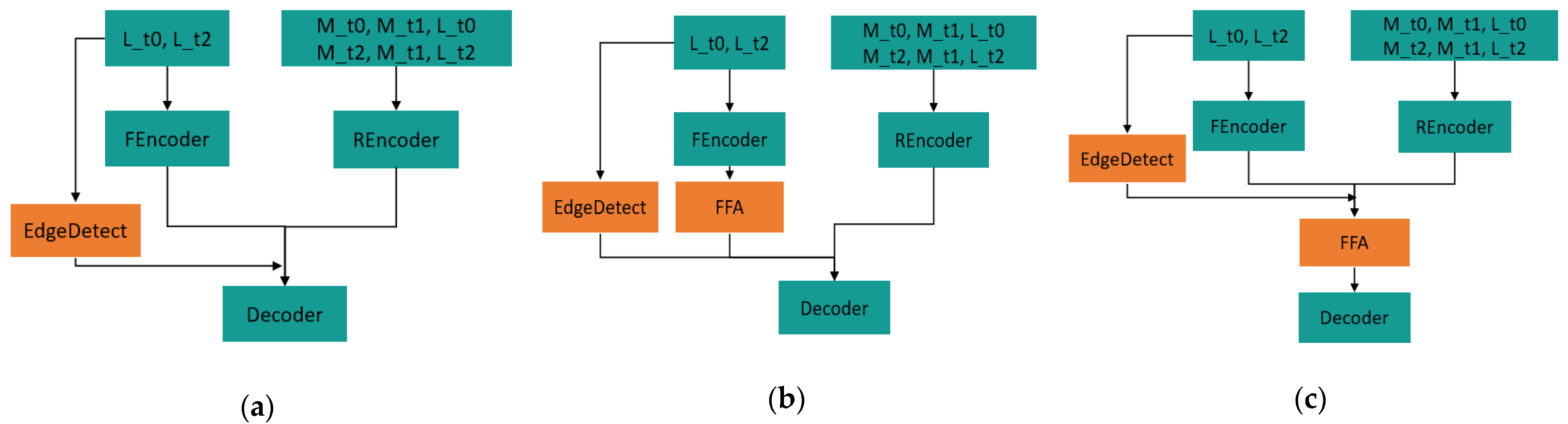
5.1. Ablation Experiment
5.2. Discussion
6. Conclusions
Author Contributions
Funding
Data Availability Statement
Conflicts of Interest
Abbreviations
| STF-EGFA | Spatiotemporal fusion network with edge-guided feature attention |
| CNN | Convolutional neural network |
| MODIS | Moderate Resolution Imaging Spectrometer |
| STARFM | Spatial and temporal adaptive reflectance fusion model |
| STRUM | Spatiotemporal restraint unmixing |
| STAARCH | Spatiotemporal adaptive algorithm for mapping reflectance change |
| FIT-FC | Fitting, and residual compensation |
| LR | Linear regression |
| FSDAF | Flexible spatiotemporal data fusion |
| GPU | Graphics Processing Units |
| CSSF | Compression sensing for spatiotemporal fusion |
| SPSTFM | Spatiotemporal reflectance fusion via sparse representation |
| HSTAFM | Hierarchical spatiotemporal adaptive fusion model |
| BiaSTF | Spatiotemporal fusion model driven by sensor bias |
| ASPP | Atrous spatial pyramid pooling |
| DCSTFN | Deep convolutional spatiotemporal fusion network |
| FA | Feature attention |
| PA | Pixel attention |
| CA | Channel attention |
| SAM | Spectral angle mapper |
| PSNR | Peak signal-to-noise ratio |
| CC | Correlation coefficient |
| SSIM | Structural similarity |
| RMSE | Root mean square error |
References
- Ghamisi, P.; Rasti, B.; Yokoya, N.; Wang, Q.; Hofle, B.; Bruzzone, L.; Bovolo, F.; Chi, M.; Anders, K.; Gloaguen, R.; et al. Multisource and Multitemporal Data Fusion in Remote Sensing: A Comprehensive Review of the State of the Art. IEEE Geosci. Remote Sens. Mag. 2019, 7, 6–39. [Google Scholar] [CrossRef] [Green Version]
- Liu, S.; Marinelli, D.; Bruzzone, L.; Bovolo, F. A Review of Change Detection in Multitemporal Hyperspectral Images: Current Techniques, Applications, and Challenges. IEEE Geosci. Remote Sens. Mag. 2019, 7, 140–158. [Google Scholar] [CrossRef]
- Chen, B.; Huang, B.; Xu, B. Comparison of Spatiotemporal Fusion Models: A Review. Remote Sens. 2015, 7, 1798–1835. [Google Scholar] [CrossRef] [Green Version]
- Zhu, X.; Cai, F.; Tian, J.; Williams, T.K.-A. Spatiotemporal Fusion of Multisource Remote Sensing Data: Literature Survey, Taxonomy, Principles, Applications, and Future Directions. Remote Sens. 2018, 10, 527. [Google Scholar] [CrossRef] [Green Version]
- Javan, F.D.; Samadzadegan, F.; Mehravar, S.; Toosi, A.; Khatami, R.; Stein, A. A review of image fusion techniques for pan-sharpening of high-resolution satellite imagery. ISPRS J. Photogramm. Remote Sens. 2021, 171, 101–117. [Google Scholar] [CrossRef]
- Peng, Y.; Li, W.; Luo, X.; Du, J.; Gan, Y.; Gao, X. Integrated fusion framework based on semicoupled sparse tensor factorization for spatio-temporal–spectral fusion of remote sensing images. Inf. Fusion 2021, 65, 21–36. [Google Scholar] [CrossRef]
- Chiesi, M.; Battista, P.; Fibbi, L.; Gardin, L.; Pieri, M.; Rapi, B.; Romani, M.; Sabatini, F.; Maselli, F. Spatio-temporal fusion of NDVI data for simulating soil water content in heterogeneous Mediterranean areas. Eur. J. Remote Sens. 2019, 52, 88–95. [Google Scholar] [CrossRef] [Green Version]
- Wang, T.; Tang, R.; Li, Z.-L.; Tang, B.; Wu, H.; Jiang, Y.; Liu, M. A Comparison of Two Spatio-Temporal Data Fusion Schemes to Increase the Spatial Resolution of Mapping Actual Evapotranspiration. In Proceedings of the IGARSS 2018—2018 IEEE International Geoscience and Remote Sensing Symposium, Valencia, Spain, 22–27 July 2018; pp. 7023–7026. [Google Scholar]
- Yang, X.; Lo, C.P. Using a time series of satellite imagery to detect land use and land cover changes in the Atlanta, Georgia metropolitan area. Int. J. Remote Sens. 2002, 23, 1775–1798. [Google Scholar] [CrossRef]
- He, S.; Shao, H.; Xian, X.; Zhang, S.; Zhong, J.; Qi, J. Extraction of Abandoned Land in Hilly Areas Based on the Spatio-Temporal Fusion of Multi-Source Remote Sensing Images. Photogramm. Eng. Remote Sens. 2021, 13, 3956. [Google Scholar] [CrossRef]
- Huang, B.; Zhao, Y. Research Status and Prospect of Spatiotemporal Fusion of Multi-source Satellite Remote Sensing Imagery. Acta Geod. Cartogr. Sin. 2017, 46, 1492–1499. [Google Scholar]
- Li, J.; Li, Y.; He, L.; Chen, J.; Plaza, A. Spatio-temporal fusion for remote sensing data: An overview and new benchmark. China Inf. 2020, 63, 140301. [Google Scholar] [CrossRef] [Green Version]
- Yang, G.Q.; Liu, H.; Zhong, X.W.; Chen, L.; Qian, Y.R. Temporal and spatial fusion of remote sensing images: A comprehensive revie. Comput. Eng. Appl. 2022, 58, 27–40. [Google Scholar]
- Gao, F.; Masek, J.; Schwaller, M.; Hall, F. On the Blending of the Landsat and MODIS Surface Reflectance: Predicting Daily Landsat Surface Reflectance. IEEE Trans. Geosci. Remote Sens. 2006, 44, 2207–2218. [Google Scholar]
- Zhu, X.; Chen, J.; Gao, F.; Chen, X.; Masek, J.G. An enhanced spatial and temporal adaptive reflectance fusion model for complex heterogeneous regions. Remote Sens. Environ. 2010, 114, 2610–2623. [Google Scholar] [CrossRef]
- Hilker, T.; Wulder, M.A.; Coops, N.C.; Linke, J.; McDermid, G.; Masek, J.G.; Gao, F.; White, J.C. A new data fusion model for high spatial- and temporal-resolution mapping of forest disturbance based on Landsat and MODIS. Remote Sens. Environ. 2009, 113, 1613–1627. [Google Scholar] [CrossRef]
- Gevaert, C.M.; Garcia-Haro, F.J. A comparison of STARFM and an unmixing-based algorithm for Landsat and MODIS data fusion. Remote Sens. Environ. 2015, 156, 34–44. [Google Scholar] [CrossRef]
- Wang, Q.; Atkinson, P.M. Spatio-temporal fusion for daily Sentinel-2 images. Remote Sens. Environ. 2018, 204, 31–42. [Google Scholar] [CrossRef] [Green Version]
- Zhu, X.; Helmer, E.H.; Gao, F.; Liu, D.; Chen, J.; Lefsky, M.A. A flexible spatiotemporal method for fusing satellite images with different resolutions. Remote Sens. Environ. Interdiscip. J. 2016, 172, 165–177. [Google Scholar] [CrossRef]
- Shi, C.; Wang, X.; Zhang, M.; Liang, X.; Niu, L.; Han, H.; Zhu, X. A Comprehensive and Automated Fusion Method: The Enhanced Flexible Spatiotemporal DAta Fusion Model for Monitoring Dynamic Changes of Land Surface. Appl. Sci. 2019, 9, 3693. [Google Scholar] [CrossRef] [Green Version]
- Liu, M.; Yang, W.; Zhu, X.; Chen, J.; Chen, X.; Yang, L.; Helmer, E.H. An Improved Flexible Spatiotemporal DAta Fusion (IFSDAF) method for producing high spatiotemporal resolution normalized difference vegetation index time series. Remote Sens. Environ. 2019, 227, 74–89. [Google Scholar] [CrossRef]
- Bernabe, S.; Martin, G.; Nascimento, J.M.P.; Bioucas-Dias, J.M.; Plaza, A.; Silva, V. Parallel Hyperspectral Coded Aperture for Compressive Sensing on GPUs. IEEE J. Sel. Top. Appl. Earth Obs. Remote Sens. 2016, 9, 932–944. [Google Scholar] [CrossRef]
- Gao, H.; Zhu, X.; Guan, Q.; Yang, X.; Yao, Y.; Zeng, W.; Peng, X. cuFSDAF: An Enhanced Flexible Spatiotemporal Data Fusion Algorithm Parallelized Using Graphics Processing Units. IEEE Trans. Geosci. Remote Sens. 2021, 60, 1–16. [Google Scholar] [CrossRef]
- Huang, B.; Song, H. Spatiotemporal Reflectance Fusion via Sparse Representation. IEEE Trans. Geosci. Remote Sens. 2012, 50, 3707–3716. [Google Scholar] [CrossRef]
- Li, L.; Liu, P.; Wu, J.; Wang, L.; He, G. Spatiotemporal Remote-Sensing Image Fusion with Patch-Group Compressed Sensing. IEEE Access 2020, 8, 209199–209211. [Google Scholar] [CrossRef]
- Chen, B.; Huang, B.; Xu, B. A hierarchical spatiotemporal adaptive fusion model using one image pair. Int. J. Digit. Earth 2016, 10, 639–655. [Google Scholar] [CrossRef]
- Li, D.; Li, Y.; Yang, W.; Ge, Y.; Han, Q.; Ma, L.; Chen, Y.; Li, X. An Enhanced Single-Pair Learning-Based Reflectance Fusion Algorithm with Spatiotemporally Extended Training Samples. Remote Sens. 2018, 10, 1207. [Google Scholar] [CrossRef] [Green Version]
- Lei, D.; Ran, G.; Zhang, L.; Li, W. A spatiotemporal fusion method based on multiscale feature extraction and spatial channel attention mechanism. Remote Sens. 2022, 14, 461. [Google Scholar] [CrossRef]
- Li, W.; Zhang, X.; Peng, Y.; Dong, M. DMNet: A network architecture using dilated convolution and multiscale mechanisms for spatiotemporal fusion of remote sensing images. IEEE Sens. J. 2020, 20, 12190–12202. [Google Scholar] [CrossRef]
- Song, H.; Liu, Q.; Wang, G.; Hang, R.; Huang, B. Spatiotemporal Satellite Image Fusion Using Deep Convolutional Neural Networks. IEEE J. Sel. Top. Appl. Earth Obs. Remote Sens. 2018, 11, 821–829. [Google Scholar] [CrossRef]
- Li, Y.; Liu, C.; Yan, L.; Li, J.; Plaza, A.; Li, B. A New Spatio-Temporal Fusion Method for Remotely Sensed Data Based on Convolutional Neural Networks. In Proceedings of the IGARSS 2019—2019 IEEE International Geoscience and Remote Sensing Symposium, Yokohama, Japan, 28 July–5 August 2019; p. 835. [Google Scholar]
- Li, Y.; Li, J.; He, L.; Chen, J.; Plaza, A. A new sensor bias-driven spatio-temporal fusion model based on convolutional neural networks. China Inf. 2020, 63, 140302. [Google Scholar] [CrossRef] [Green Version]
- Liu, X.; Deng, C.; Chanussot, J.; Hong, D.; Zhao, B. StfNet: A Two-Stream Convolutional Neural Network for Spatiotemporal Image Fusion. IEEE Trans. Geosci. Remote Sens. 2019, 57, 6552–6564. [Google Scholar] [CrossRef]
- Chen, Y.; Shi, K.; Ge, Y.; Zhou, Y. Spatiotemporal Remote Sensing Image Fusion Using Multiscale Two-Stream Convolutional Neural Networks. IEEE Trans. Geosci. Remote Sens. 2021, 60, 4402112. [Google Scholar] [CrossRef]
- Jia, D.; Song, C.; Cheng, C.; Shen, S.; Ning, L.; Hui, C. A Novel Deep Learning-Based Spatiotemporal Fusion Method for Combining Satellite Images with Different Resolutions Using a Two-Stream Convolutional Neural Network. Remote Sens. 2020, 12, 698. [Google Scholar] [CrossRef] [Green Version]
- Tan, Z.; Yue, P.; Di, L.; Tang, J. Deriving High Spatiotemporal Remote Sensing Images Using Deep Convolutional Network. Remote Sens. 2018, 10, 1066. [Google Scholar] [CrossRef] [Green Version]
- Tan, Z.; Di, L.; Zhang, M.; Guo, L.; Gao, M. An Enhanced Deep Convolutional Model for Spatiotemporal Image Fusion. Remote Sens. 2019, 11, 2898. [Google Scholar] [CrossRef] [Green Version]
- Liu, J.; Fan, X.; Jiang, J.; Liu, R.; Luo, Z. Learning a Deep Multi-scale Feature Ensemble and an Edge-attention Guidance for Image Fusion. IEEE Trans. Circuits Syst. Video Technol. 2021, 32, 105–119. [Google Scholar] [CrossRef]
- Qin, X.; Wang, Z.; Bai, Y.; Xie, X.; Jia, H. FFA-Net: Feature Fusion Attention Network for Single Image Dehazing. Proc. AAAI Conf. Artif. Intell. 2020, 34, 11908–11915. [Google Scholar] [CrossRef]
- Lim, B.; Son, S.; Kim, H.; Nah, S.; Lee, K.M. Enhanced Deep Residual Networks for Single Image Super-Resolution. In Proceedings of the 2017 IEEE Conference on Computer Vision and Pattern Recognition Workshops (CVPRW), Honolulu, HI, USA, 21–26 July 2017; pp. 1132–1140. [Google Scholar]
- Yuhas, R.H.; Goetz, A.F.H.; Boardman, J.W. Discrimination among semi-arid landscape endmembers using the Spectral Angle Mapper (SAM) algorithm. In Proceedings of the Twenty-Fourth Lunar and Planetary Science Conference, Pasadena, CA, USA, 1–5 June 1992; pp. 147–149. [Google Scholar]
- Huynh-Thu, Q.; Ghanbari, M. Scope of validity of PSNR in image/video quality assessment. Electron. Lett. 2008, 44, 800–801. [Google Scholar] [CrossRef]
- Alparone, L.; Wald, L.; Chanussot, J.; Thomas, C.; Gamba, P.; Bruce, L.M. Comparison of Pansharpening Algorithms: Outcome of the 2006 GRS-S Data Fusion Contest. IEEE Trans. Geosci. Remote Sens. 2007, 45, 3012–3021. [Google Scholar] [CrossRef] [Green Version]
- Wang, Z.; Bovik, A.C.; Sheikh, H.R.; Simoncelli, E.P. Image Quality Assessment: From Error Visibility to Structural Similarity. IEEE Trans. Image Process. 2004, 13, 600–612. [Google Scholar] [CrossRef] [Green Version]
- Li, W.; Cao, D.; Peng, Y.; Yang, C. MSNet: A Multi-Stream Fusion Network for Remote Sensing Spatiotemporal Fusion Based on Transformer and Convolution. Remote Sens. 2021, 13, 3724. [Google Scholar] [CrossRef]


| Dataset | Image Size | Experimental Image Size | Experimental Image Pairs | Experimental Image Time Span | Main Change Types |
|---|---|---|---|---|---|
| AHB | 2480 × 2800 × 6 | 2432 × 2432 × 6 | 27 | 30 May 2013–6 December 2018 | Ar Horqin Banner of Inner Mongolia province |
| Tianjin | 2100 × 1970 × 6 | 1920 × 1920 × 6 | 27 | 1 September 2013–18 September 2019 | Tianjin city |
| Daxing | 1640 × 1640 × 6 | 1536 × 1536 × 6 | 27 | 1 September 2013–1 August 2019 | Daxing district of Beijing |
| Method | SAM ↓ * | PSNR ↑ | CC ↑ | SSIM ↑ | RMSE ↓ |
|---|---|---|---|---|---|
| STARFM | 0.339 | 22.220 | 0.351 | 0.687 | 22.946 |
| FSDAF | 0.324 | 22.412 | 0.524 | 0.681 | 20.444 |
| EDCSTFN | 0.101 | 28.147 | 0.433 | 0.840 | 11.368 |
| STF-EGFA | 0.092 | 28.751 | 0.485 | 0.869 | 9.633 |
| Method | SAM ↓ | PSNR ↑ | CC ↑ | SSIM ↑ | RMSE ↓ |
|---|---|---|---|---|---|
| STARFM | 0.375 | 17.462 | 0.268 | 0.589 | 53.019 |
| FSDAF | 0.240 | 20.261 | 0.438 | 0.632 | 32.500 |
| EDCSTFN | 0.110 | 28.554 | 0.761 | 0.772 | 9.536 |
| STF-EGFA | 0.089 | 30.327 | 0.876 | 0.844 | 7.794 |
| Method | SAM ↓ | PSNR ↑ | CC ↑ | SSIM ↑ | RMSE ↓ |
|---|---|---|---|---|---|
| STARFM | 0.090 | 27.942 | 0.731 | 0.805 | 10.221 |
| FSDAF | 0.088 | 28.941 | 0.776 | 0.811 | 9.144 |
| EDCSTFN | 0.073 | 30.766 | 0.841 | 0.826 | 7.426 |
| STF-EGFA | 0.065 | 31.650 | 0.882 | 0.860 | 6.689 |
| Method | SAM ↓ | PSNR ↑ | CC ↑ | SSIM ↑ | RMSE ↓ |
|---|---|---|---|---|---|
| EDCSTFN | 0.073 | 30.766 | 0.841 | 0.826 | 7.426 |
| Only edge | 0.062 | 31.561 | 0.877 | 0.858 | 6.752 |
| Edge-FA-encoder | 0.063 | 31.585 | 0.882 | 0.860 | 6.748 |
| Edge-FA-decoder | 0.065 | 31.650 | 0.882 | 0.860 | 6.689 |
Publisher’s Note: MDPI stays neutral with regard to jurisdictional claims in published maps and institutional affiliations. |
© 2022 by the authors. Licensee MDPI, Basel, Switzerland. This article is an open access article distributed under the terms and conditions of the Creative Commons Attribution (CC BY) license (https://creativecommons.org/licenses/by/4.0/).
Share and Cite
Cheng, F.; Fu, Z.; Tang, B.; Huang, L.; Huang, K.; Ji, X. STF-EGFA: A Remote Sensing Spatiotemporal Fusion Network with Edge-Guided Feature Attention. Remote Sens. 2022, 14, 3057. https://doi.org/10.3390/rs14133057
Cheng F, Fu Z, Tang B, Huang L, Huang K, Ji X. STF-EGFA: A Remote Sensing Spatiotemporal Fusion Network with Edge-Guided Feature Attention. Remote Sensing. 2022; 14(13):3057. https://doi.org/10.3390/rs14133057
Chicago/Turabian StyleCheng, Feifei, Zhitao Fu, Bohui Tang, Liang Huang, Kun Huang, and Xinran Ji. 2022. "STF-EGFA: A Remote Sensing Spatiotemporal Fusion Network with Edge-Guided Feature Attention" Remote Sensing 14, no. 13: 3057. https://doi.org/10.3390/rs14133057
APA StyleCheng, F., Fu, Z., Tang, B., Huang, L., Huang, K., & Ji, X. (2022). STF-EGFA: A Remote Sensing Spatiotemporal Fusion Network with Edge-Guided Feature Attention. Remote Sensing, 14(13), 3057. https://doi.org/10.3390/rs14133057