Article

3D Rock Structure Digital Characterization Using Airborne LiDAR and Unmanned Aerial Vehicle Techniques for Stability Analysis of a Blocky Rock Mass Slope

1
State Key Laboratory of Geohazard Prevention and Geoenvironment Protection, Chengdu University of Technology, Chengdu 610059, China
2
Institute of Applied Geosciences, Graz University of Technology, 8010 Graz, Austria
*
Author to whom correspondence should be addressed.
Remote Sens. 2022, 14(13), 3044; https://doi.org/10.3390/rs14133044
Submission received: 9 May 2022 / Revised: 22 June 2022 / Accepted: 22 June 2022 / Published: 24 June 2022

Abstract

:
Airborne light detection and ranging (LiDAR) and unmanned aerial vehicle-structure from motion (UAV-SfM) provide point clouds with unprecedented resolution and accuracy that are well suited for the digital characterization of rock outcrops where direct contact measurements cannot be obtained due to terrain or safety constraints. Today, however, how to better apply these techniques to the practice of geostructural analysis is a topic of research that must be further explored. This study presents a processing procedure for extracting three-dimensional (3D) rock structure parameters directly from point clouds using open-source software and a three-dimensional distinct element code-assisted (3DEC) simulation of slope failure based on carbonate rock cliffs in the Jiuzhaigou Scenic Area. The procedure involves (1) processing point clouds obtained with different remote sensing techniques; (2) using the Hough transform to estimate normals for the hue, saturation, and value (HSV) rendering of unstructured point clouds; (3) automatically clustering and extracting the set-based point clouds; (4) estimating set-based geometric parameters; and (5) performing a subsequent stability analysis based on rock structure parameters. The results show that integrating different remote sensing techniques and rock structure computing can provide a quick way for slope engineers to assess the safety of blocky rock masses.

Graphical Abstract

1. Introduction

Rock slopes are usually formed by primary (i.e., bedding planes) or secondary (i.e., joints, faults) discontinuities. Rock mass behaviour is controlled by intact rock properties and by the discontinuities present in the rock mass. The generation of rock mass anisotropy by discontinuities increases the complexity of the gradual failure of rock slopes [1,2]. Detailed and accurate characterization of set-based in situ discontinuities is therefore particularly important.
Traditional contact-based field measurement methods, such as scanline and window mapping of near-vertical rock slope faces, are particularly complex and inaccessible [3,4,5,6]. Thus, the measured data are not always representative of the whole investigated slope due to the acquisition of rock structure information in the few accessible rock outcrops [7,8,9,10,11,12,13,14]. Hazardous conditions, especially in rugged karst areas, may preclude direct contact measurements. The discontinuities that exist in carbonate rock outcrops are generally accompanied by dissolution, weathering, and karst processes, making measurements and analyses more complex [15,16,17,18,19]. Combining field monitoring data allows the identification of complex hydrological processes involving moisture information in surface soils and shallow groundwater systems developed in limestone bedrock that control conditions that may predispose slopes to landslides [20,21]. Currently, there is great interest in the application of terrestrial or airborne LiDAR and close-range photogrammetry techniques for rock slope investigations and the accurate detection of location-dependent rock structures from point clouds. For instance, several works have illustrated the main advantages and limitations of using the different remote sensing techniques described above to detect, characterize, and monitor rockfall sources at the local outcrop scale or regional scale [22,23,24]. The relevant parameters of discontinuities required for evaluating the stability of slopes and kinematic failure mode analysis of massive rock masses are extracted from the acquired point cloud by using semiautomatic or fully automatic methods. Several researchers have proposed different solutions to derive an irregular triangular mesh model from a 3D point cloud and then calculate the best fit of the plane to identify the discontinuity sets [25,26,27]. Another approach is to acquire 3D rock structure information directly from raw or processed 3D point clouds [28,29,30,31]. As introduced above, the methods of acquiring rock structure information by different remote sensing techniques have been greatly developed in recent years. However, how to better apply these techniques to the practice of geological engineering requires further research. This is especially true in environments with complex geological structures and high geological risks, which pose a serious threat to human activities and infrastructure in places of high tourist attraction. International experience, e.g., [32], has shown that the location-dependent topographical details and the spatial organization of discontinuities in the formation of kinematically unstable blocks are indispensable information both for the risk assessment of rock slopes and for rehabilitation measures. In this article, we show how to process remote sensing data to obtain parameters of slope topography and rock mass structure, and use them for slope stability evaluation in Jiuzhaigou County, Sichuan Province, China.
On 8 August 2017, a magnitude 7.0 earthquake struck Jiuzhaigou County, triggering thousands of geological disasters, mainly small-scale rockfalls and rockslides, and causing the Jiuzhaigou Scenic Area to enter a three-year closure. The background of the study area is explained in the second section. Due to the inability to conduct on-site rock structure measurements on near-vertical slopes with heights exceeding hundreds of metres, we surveyed the typical dangerous rock masses and surrounding slopes using UAV and aerial laser scanning (ALS), respectively. The applied digital acquisition based on ALS and UAV-SfM is presented in the third section, which mainly covers the survey of 3D point clouds of different scales from the carbonate cliffs at the entrance of the Jiuzhaigou tourist attraction. The methods for extracting rock structures, based on our recent developments and the Discontinuity Set Extractor (DSE) software [33], are also explained in the third section. Finally, we use the extracted 3D rock structure parameters for rock slope stability analysis and as input for 3D distinct element analysis to simulate the potential movement of the dangerous rock mass. The results of this study, especially the proven effectiveness of our open-source procedure for processing rock structure information applied to block stability assessment, contribute to risk assessment related to possible rockfalls and secondary geohazards in the Jiuzhaigou Scenic Area.

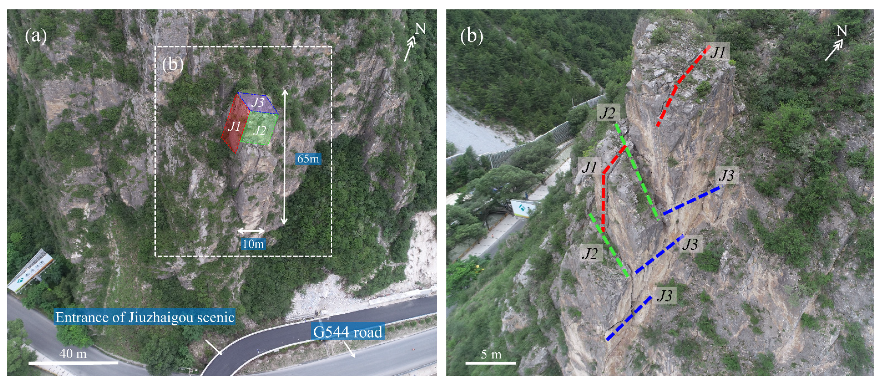
2. Study Site Description

The Jiuzhaigou tourist attraction is located in the north of Sichuan province, approximately 400 km away from Chengdu (Figure 1a). Three years after the Ms 7.0 earthquake on 8 August 2017, the Jiuzhaigou Scenic Area is now open to the public again. Shallow landslides, collapses, and rockfalls frequently occurred in this area after the earthquake, raising concerns about the safe operation of the G544 national road to the scenic area [34,35]. The nearly erect slope studied is located north of the entrance of the scenic spot, next to the G544 national road (Figure 1b). The approximately 1000-metre-high slope is subvertical (ranging between 2070 m and 3100 m a.s.l.). Although it was impossible for us to conduct field-based measurements of the complete fracture network of the slope, which is necessary to investigate how the in situ 3D rock structure controls slope stability, we were able to establish the spatial distribution between the main discontinuity sets through different remote sensing techniques.
The terrain of the study area is dominated by tectonically controlled steep valleys. Through the analysis of geological data, the large-scale WNW-directed strike-slip Tazang fault and Wenxian fault were detected (Figure 2). The Minjiang fault is a thrust fault that generally strikes N–S and extends for approximately 100 km [36,37]. The overall tectonic characteristics of Jiuzhaigou Valley are basically the same as those of SSW–NNE or WNW–ESE, which fully indicates the controlling effect of tectonic development. The main strata of the studied slope have the following sequences from the top down: (1) the massive limestone of the Permian Xiawula (Dx) and Yiguigou (Dcy) Formations, (2) the bioclastic limestone and dolomitic limestone of the Carboniferous Minhe (Cm1 and Cm2) and Daguanshan (Cpd) Formations, and (3) the sandstone and slate of the Triassic Zhaga (Tzg) and Zagunao (Tz) Formations.
Field investigation and preliminary analysis showed that the typical dangerous rock mass at the slope of the newly built road at the entrance of the scenic spot is formed by three main joint sets (Figure 3a). The volume of this dangerous rock mass was evaluated as 3000–4000 m3; its detachment, with sliding and toppling phenomena, would involve at first the entrance of the scenic spot and, afterward, the G544 road directly. As shown in Figure 3b, three highly persistent discontinuity sets were identified based on the field documentation. Due to the inaccessibility and danger of the slope, it was difficult to accurately measure their orientation of the discontinuities with a compass in the field. This is one of the reasons why we decided to use airborne LiDAR combined with the UAV close-range photogrammetry technique to determine the local rock structure parameters. Joint set J1 cuts obliquely into the slope, with a dip direction of 200–230° and a dip angle of 70–80°. Based on its long-term persistence and orientation parallel to the Baishui River, J1 is clearly controlled by the Tazang fault. Joint set J2 is persistent and forms the slope face with a nearly east–west strike, dipping to the south with a dip angle of 70–85°. Together, J1 and J2 form the boundary of the dangerous rock mass. Joint set J3 is another discontinuity group cutting obliquely into the slope, with a dip direction of 40–60° and a dip of 20–40°. The low-angle J3 discontinuity group plays a decisive role in the stability of rock outcrops.

3. Data and Methods

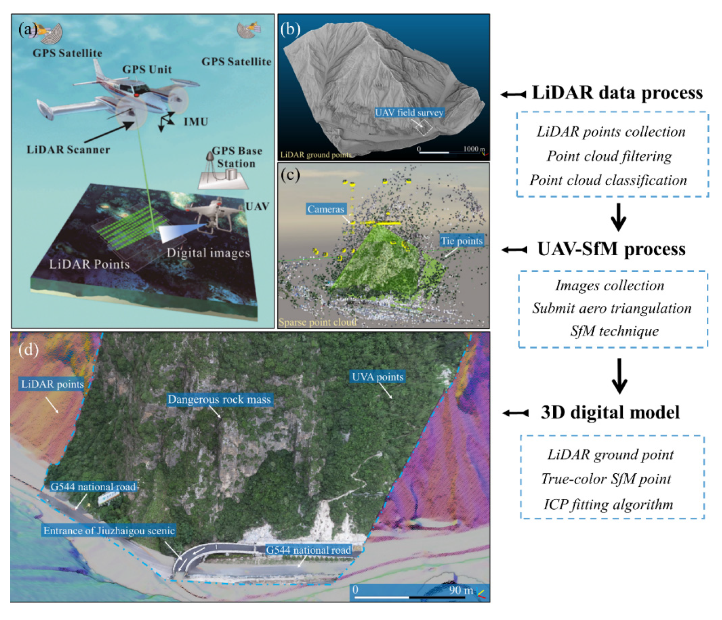
3.1. 3D Point Cloud Acquisition and Processing

For the dangerous rock mass at the entrance of the scenic spot, a detailed investigation was carried out using UAV, and the whole slope was scanned by airborne LiDAR. The purpose of using these two remote sensing techniques was to obtain comprehensive structural parameters of the investigated slope (Figure 4). Although the limited accessibility of the terrain makes it difficult to conduct the direct mapping of some rock structure parameters, such as set-based orientation, spacing, and persistence, the deployed digital acquisition based on ALS and UAV-SfM in this study overcame this difficulty very well.

3.2. Airborne LiDAR Data

The large-scale airborne LiDAR dataset was collected on 13 August 2018, one year after the earthquake. Airborne LiDAR enables regional measurements with an orthographic view and penetrates vegetation to minimize occluded areas in alpine terrains. An AS350 helicopter was equipped with a Leica ALS80-HP airborne LiDAR system suitable for high mountain areas to obtain point cloud data with echo information (Figure 4a). The specifications of the LiDAR system are shown in Table 1. During the measurement process, the flight platform performed a varying-altitude flight within 1500–3500 m to realize laser measurement and synchronously acquire digital photos. At the same time, multiple georeferenced ground control points (GCP) and global positioning system (GPS) receivers were set up around the study area. The airborne LiDAR datasets effectively filter out vegetation and provide high-precision real topography to help detect rock structures around investigated slopes. By using the TerraScan module in Terrasolid software, various types of point clouds were classified by using related macros, and finally, a high-resolution ground point cloud was obtained (Figure 4b). The LiDAR ground point cloud had a mean point spacing of 0.5 m and was georeferenced in the EPSG: 32648 WGS84/UTM zone 49N (data: World Geodetic System 1984) metric coordinate system.

3.3. UAV-SfM Data

A scaled and oriented SfM point cloud model was reconstructed using UAV photogrammetry for the dangerous rock mass found in the field survey above the scenic entrance road. The relevant parameters of the DJI Phantom 4 Real Time Kinematic (RTK) system are shown in Table 1. Considering that the rock outcrops are inaccessible and dangerous, a total of 377 high-resolution photographs with coordinate information were obtained under manual control via overlapping. The DJI was equipped with a global navigation satellite system/inertial measurement unit (GNSS/IMU) and network RTK modules, and all the acquired images were georeferenced in a WGS84/UTM zone 49N metric coordinate system. By ContextCapture, we generated a true-colour point cloud and a reality model using a series of high-resolution photographs with coordinate information obtained by DJI (Figure 4c). The processing steps are summarized below, which were completed on a graphics workstation with a 2.20 GHz CPU and 128 GB RAM. Aerial triangulation fully calibrated all images by automatically identifying the relative position and orientation of each image. The orientation and magnitude of the camera position uncertainty calculated by aerial triangulation are shown in Table 2. The final aerial triangulation results show that 375 of the 377 images were calibrated and that the ground coverage area was 0.131 km2. The reconstructed sparse (low-density) 3D point cloud model (Figure 4c) had an average ground resolution of 19.18 mm/pixel and a reprojection error (RMS) of 0.54 pixels. There were a total of 56,203 tie points and a median of 44,924 key points per image. A dense point cloud with point sampling of approximately 0.019 m was generated. The final true-colour point cloud model was exported as an LAS file, and each point was georeferenced in the set coordinate system (X = east, Y = north, positive Z = up). All points were assigned red, green, and blue (RGB) colour values. The alignment was performed using the open-source software CloudCompare v.2.11. Based on the airborne LiDAR data shown in Figure 4d, the SfM point cloud was matched by manually selecting multiple pairs of common points and then by adopting the iterative closest point (ICP) best-fitting algorithm [38,39,40].

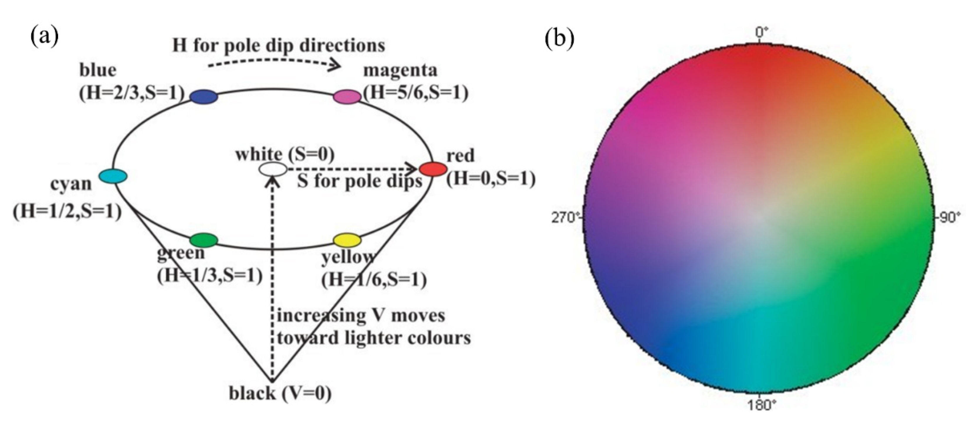
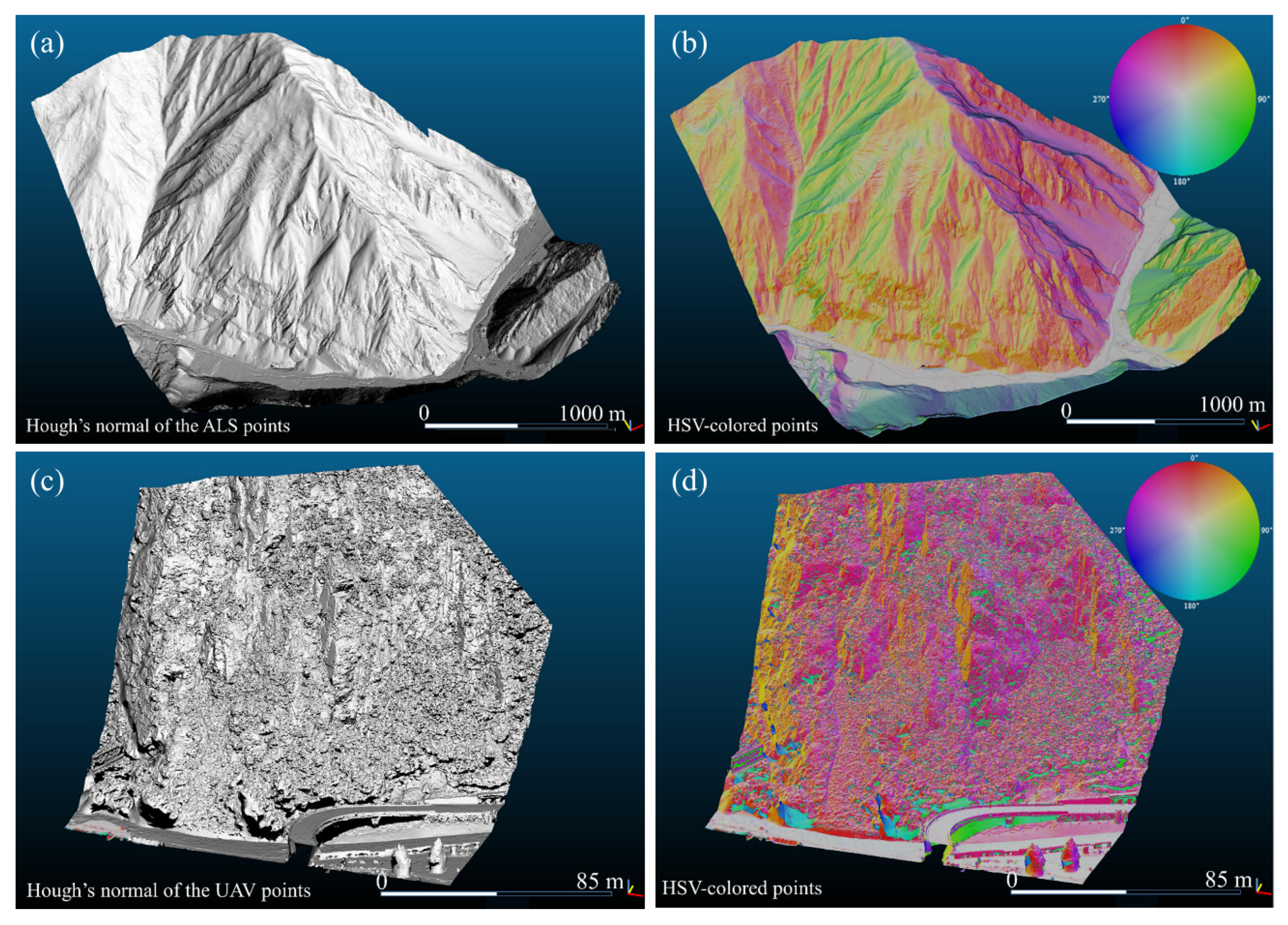
3.4. Extraction of Rock Structure from Point Clouds

As a result, to directly extract the discontinuity sets from a 3D point cloud, the normal components of each point and its nearest neighbours were first calculated. The normal components of the initial point cloud were calculated using the Hough transform algorithm in CloudCompare and were directly converted to the dip angle and dip direction of its corresponding planes. The relevant parameters used to calculate the transformed normal direction for each point are defined in Table 3. The advantage of the Hough transform for computing point normals is that millions of points can be processed, and the normal of a point on a sharp intersecting edge can be reconstructed [41].
COLTOP-3D is a software that can be intuitively used to visually identify discontinuities, faults, and cliffs in digital elevation models (DEMs) and point clouds [42,43]. The HSV-coloured point clouds facilitate visualization of the spatial distributions of set-based discontinuities [44,45]. Next, to clearly perceive and visualize 3D rock structures in point clouds, we used the open-source Python scripting language to build our HSV colour wheel for fracture normals. Once the normal components were calculated using the Hough algorithm, the point cloud data rendering was fully automated by a Python script. Hue (H) was linked to the dip direction of the normal of a discontinuity, and saturation (S) was linked to the dip angle of the normal (Figure 5a). The lightness value (V) was fixed at V = 0.75 so that the HSV wheel had uniform brightness. According to the above concept, in the HSV colour wheel for the fractures, each pole representing the orientation of a discontinuous normal was assigned a unique HSV colour. Both the dip direction and dip angle had a resolution of 1° in equal-angle and low-hemisphere projections (Figure 5b).
The third step of the open-source processing procedure was to use the R package spherical k-means to extract the main discontinuity sets based on the point cloud normal components [46,47]. This package uses the cosine angle between the vectors minus 1 as the dissimilarity judgement, clusters the normal orientations, and divides the entire point cloud into subclasses. The silhouette plot helps to identify the best number of clusters for the set-based point clouds [48]. After the clustering calculation was completed, the points assigned to the same set had similar HSV colours. The result of the set membership of each point and the HSV colour was added to a single txt file that can be visualized with CloudCompare. In the next section, the rock structure parameters such as orientation and spacing information based on the set-based point cloud are extracted by the open-source R package “RFOC” and Discontinuity Set Extractor (DSE), respectively.

4. Results

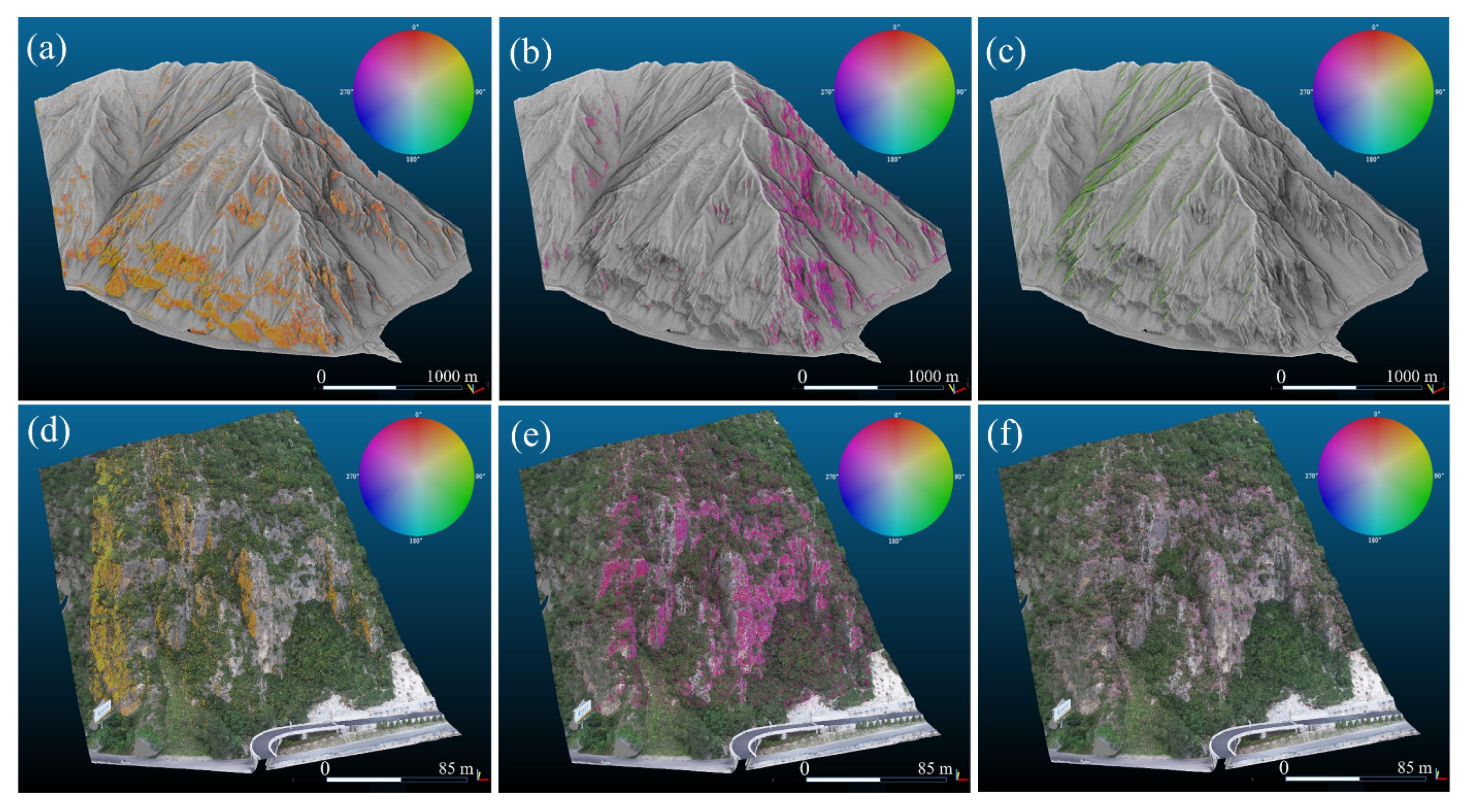
4.1. Extraction of the Set-Based Points

The initial point cloud was processed according to the above steps, and the rock structure based on Hough’s normal rendering was visualized. Figure 6a,c show the 3D digital models of the ALS and SfM point clouds processed by the Hough algorithm, respectively. In this step, the normals pointing outwards are shown as white, whereas others pointing inwards are shown as black. This rendering facilitates the detection of discontinuities and their spatial distribution relationships in the in situ slope face. A specific HSV colour was automatically assigned to the normal orientation of the corresponding point through a Python script to display the in situ rock structure more clearly. The HSV rendering shows that on the unvegetated slope, the ALS ground point cloud shows that the surface topography includes joint planes in the nonoverhanging golden and purple areas that form the main slope face (Figure 6b). For the outcrops of the dangerous rock mass, although there are noise points, such as vegetation, the golden and purple sets of high-persistence discontinuities were also detected (Figure 6d). In the following, we extracted in situ rock structures based on HSV colour-coding using an R script for clustering calculations.
The three sets of joints were directly extracted from the slope-scale ALS point cloud in Figure 6b. The golden areas in the same orientation as the Tazang fault were clustered into one set (Figure 7a). The purple areas were clustered into a second set (Figure 7b). These two main sets of joint distribution form the topography of a slope surface. The green areas constituted the third set (Figure 7c). For the outcrop-scale SfM point cloud, even with the presence of vegetation, the HSV colour distribution indicated the existence of three joint sets. The golden areas were also clustered into one set, but with a slightly higher saturation than those extracted by the ALS points (Figure 7d). The purple areas constituted the second set (Figure 7e). The third set corresponded to the light purple areas with relatively low point density (Figure 7f). The orientations of joint sets J1 and J2 were very similar between the different datasets. Notably, the orientations of the third set J3 extracted from the two datasets were significantly different. In addition, the joint set J3 obliquely cut into the slope with a dip direction of 280–290° in the ALS data but was undetectable in the SfM data. This discrepancy in results is attributable to the scale of observation for the two acquisition techniques.

4.2. Discontinuity Orientations

To calculate the set-based orientation parameters, such as the mean dip angle, dip direction, and dispersion (Fisher’s K), the extracted joint set points were processed by using the R algorithm eigen [49]. The extracted set-based point dip directions and dip angles were then plotted in a stereo projection using the R package RFOC. The main difference between the joint set orientations extracted using ALS and SfM point clouds is shown in Figure 8. According to the results of the joint sets extracted from the two datasets, the mean dip direction difference of J1 and J2 was approximately 7° and 2°, respectively. The largest difference of the discontinuity sets was in the dip angles of J1 and J2 with a discrepancy of 14° and 18°, which was steeper in the SfM data when compared with the ALS data. The most likely explanation for this difference is that the point cloud data of the subvertical rock face area and overhanging area could be accurately obtained due to the viewing direction of the airborne laser scanner. In addition, the scale of observation of the UAV photogrammetry is smaller than that of the ALS and could more accurately capture structural geometry data based on rock mass outcrop conditions. Joint set J3 was independently detected and extracted from the two point datasets. The relevant parameters of the three sets of joints extracted from the two types of point clouds are shown in Table 4. Non-persistent and fully persistent spacing was calculated using DSE’s normal spacing plugin.

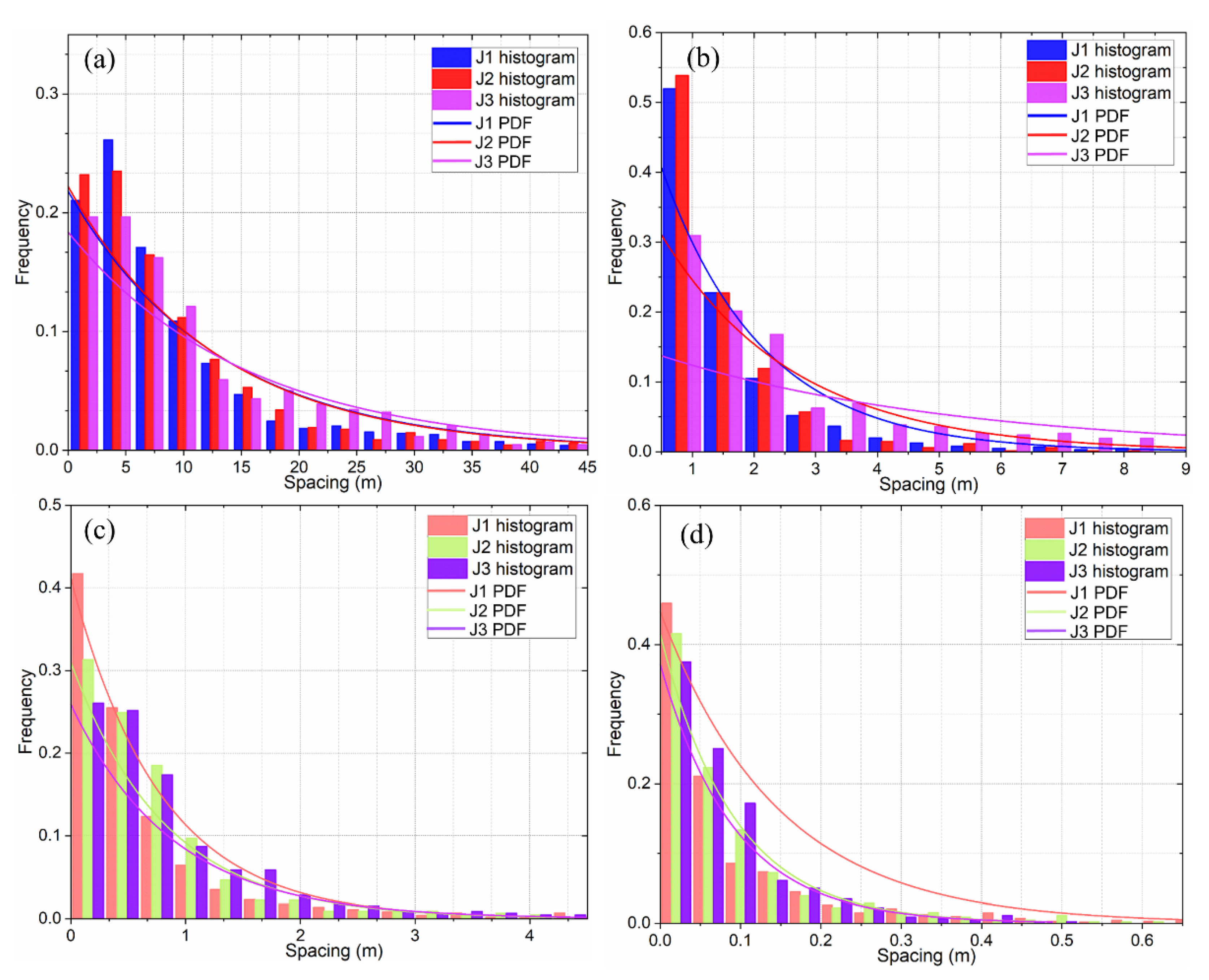
4.3. Spacing of Joint Sets

The open-source Discontinuity Set Extractor (DSE) is practical software for analysing the spacing of joint sets from 3D point cloud datasets. Non-persistent and fully persistent spacing were automatically calculated using DSE’s normal spacing plugin based on the set-based points extracted in the previous step. A histogram of the relative frequency distribution of the calculated results shows a significant difference between the two different remote measurement techniques (Figure 9). Considering the non-persistence hypothesis, the spacing values for the discontinuity sets calculated from both datasets were significantly higher than those of the persistence hypothesis. The estimated non-persistent spacings for each joint set in the ALS points varied between 2 and 45 m, with an average of approximately 14 m (Figure 9a). However, for fully persistent joints, the spacing was between approximately 1 and 9 m (Figure 9b). The results of the SfM point cloud were much lower than those calculated from the ALS technique. The spacing values of the three joint sets from the SfM point cloud were generally low, under non-persistent and persistent conditions, within the range of 0.1–4 m (Figure 9c,d). The normal spacing values of the discontinuity sets extracted from the two point clouds with DSE are reported in Table 4.

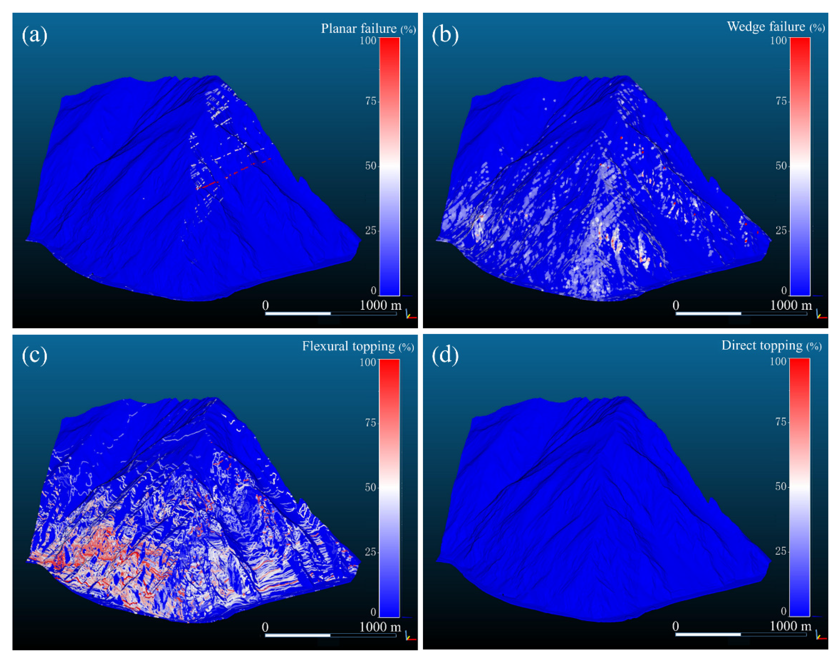
4.4. Kinematic Analysis

The outcrop-scale kinematic analysis was performed using discontinuous orientations extracted from the SfM point cloud. The purpose of this analysis was to identify the potential failure modes of a typical dangerous rock mass. This preliminary analysis was based on a stereographic technique for quickly identifying the possibility of failure of blocks by considering the geometric relationships between the slope face and joint sets. The friction angle along all discontinuities was assumed to be 30°, and the lateral limit was ±20°. Figure 10a shows that plane sliding is feasible on the J3 discontinuity set. Considering the limitation of the scale of the SfM points, wedge failure should be considered less feasible in this area, but marginally feasible at the slope scale (Figure 10b). Figure 10c highlights that the flexural toppling failure mechanism is marginally feasible on the J2 discontinuity set. The toppling failure mechanism, including direct and oblique toppling modes, is feasible on the major J2 and J3 joint sets (Figure 10d).
To identify potential modes of failures of the investigated slope, a kinematic analysis of large areas was performed through the open-source algorithm rock slope kinematic analysis (ROKA). The advantage of this method is that the effect of slope faces in different orientations can be considered and failure modes can be directly visualized on a 3D point cloud [50]. In particular, the size and spatial distribution of each extracted set of discontinuities must be provided to the algorithm as input data before execution. With the points of each set extracted as outlined above, the in situ geometric information about the discontinuities required for input can be efficiently obtained. The features of the discontinuities required for ROKA processing were mapped from the extracted set-based point cloud by CloudCompare’s compass plugin. For example, the position, size, and orientation of each discontinuity were exported as normalized Excel files required for ROKA calculation. A total of 1397 discontinuities were mapped. The ALS point cloud was subsampled to 1,227,806 points before applying the algorithm. Subsequently, the analysis was performed using a scan radius of 10 m and assuming that the friction angle and lateral limit were 30° and 20°, respectively. The results of the ROKA algorithm show the critical portions of the investigated rock slope and show the critical values of the discontinuity intersections for different potential modes of failure (Figure 11). Due to the limitation of the angle of the airborne LiDAR sensor, the points of the overhang area could not be obtained; thus, the potential failure modes of plane sliding and direct toppling were almost undetectable (Figure 11a,d). (Figure 11b) highlights that sliding along the steeper discontinuity wedge intersections of J1/J3 and J2/J3 is marginally feasible in the southeast-facing section of the investigated slope. Obviously, controlled by the Tazang fault, the flexural failure toppling mechanism is feasible in the southwest-facing sections of the investigated slope (Figure 11c).

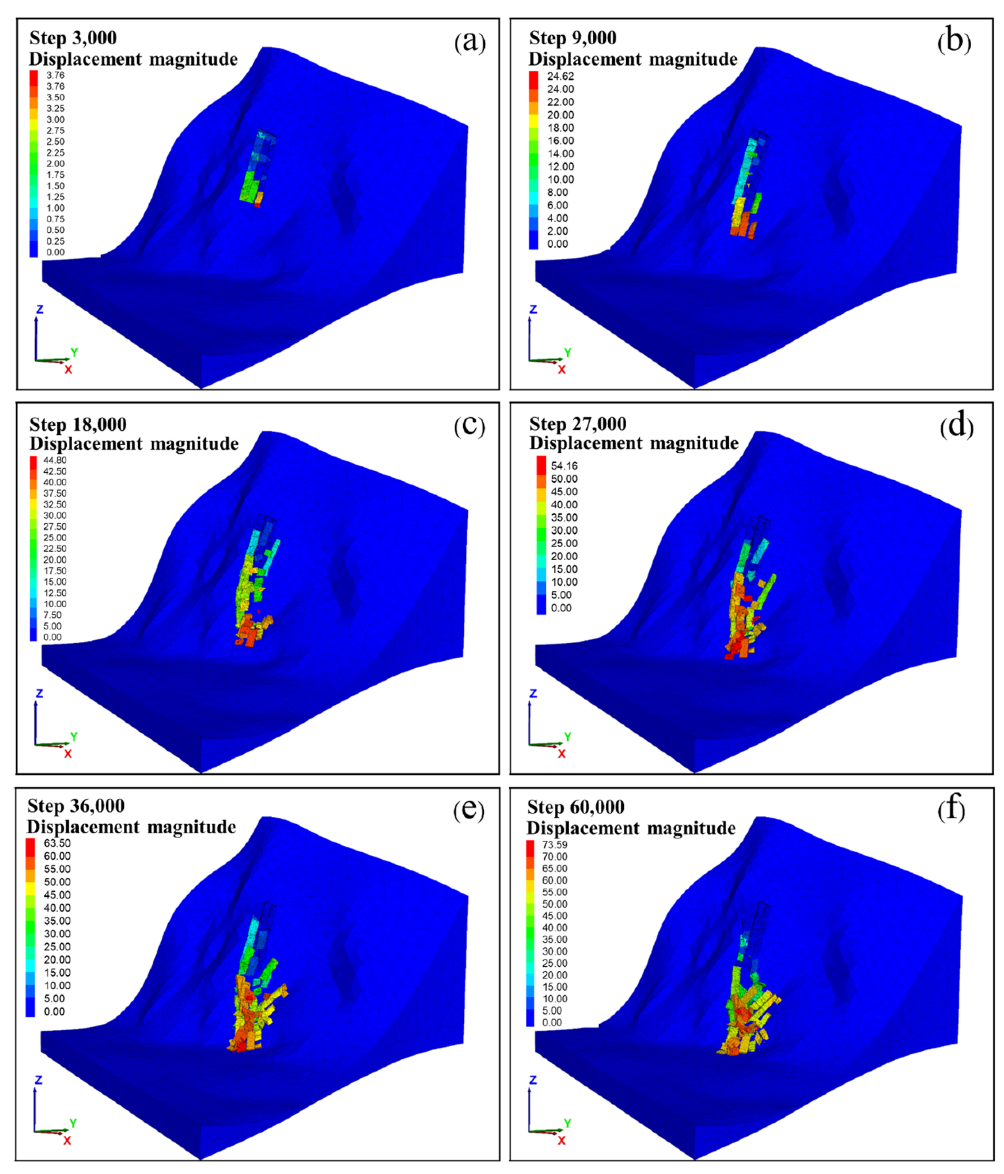
4.5. Distinct Element Modelling

The main objective of the 3DEC simulation was to evaluate the potential movement behaviour of a dangerous rock mass controlled by joint sets. In this study, we adopted the Mohr–Coulomb strength criterion and assumed that the kinematically removable blocks are regarded as rigid blocks; the input parameters are presented in Table 5. The cohesion and friction angles were derived from the results of a geomechanical investigation, and the normal and shear stiffnesses were derived from measured JRC and JCS parameters and were within the range of values reported in the literature [51,52,53]. A more realistic slope geometry was obtained from the ALS point cloud, and the plugin Griddle for Rhinoceros 6.0 was used to create volume meshes, which were then imported into 3DEC. Based on the statistical parameters from the UAV-SfM point cloud, three sets of joints were generated in the dangerous rock mass (Figure 12). In addition, the construction scope of the model was limited to the dangerous rock mass; thus, the ALS only provided the topographical details and did not use the relevant parameters extracted from it for numerical calculation. Due to the existence of obvious intact rock bridges, it could increase the cohesion and tensile strength of the initial failure surface of the dangerous rock mass [54]. Combined with the field survey, Figure 3a,b clearly show that no set was fully persistent, and a persistence factor of 0.5 was assigned to each of the three joint sets. Additionally, the results were simulated by DSE automatic calculation using the set-based non-persistent spacing extracted from the UAV dataset.
After reaching the equilibrium state, a further simulation was performed. As the 3D numerical simulation results show (Figure 13), the deformation of a dangerous rock mass consists of complex failure models rather than simple plane sliding or toppling failure. The numerical results show that after the first 9000 cycles, the right side of the dangerous rock mass exhibits a gradually increasing displacement from bottom to top (Figure 13a,b). Under the action of gravity, plane sliding failure first occurs at the bottom. Obviously, under the action of gravity, plane sliding failure occurs first at the bottom, which creates space for the next movement. As the cycle continues, it is clear that after the failure of the key block at the bottom causes the propagation to become unstable, this space is available for other blocks to move, and the blocks in the middle area gradually direct toppling to the southeast face of the slope (Figure 13c,d). During steps 36,000–60,000, the remaining blocks on the slope have the kinematics of simultaneous sliding and toppling, and some blocks are deposited on the toe of the slope (Figure 13e,f). The results of the numerical model show the whole process of dangerous rock mass deformation to failure and predict the mechanism of failure and location of the unstable portion of the slope.

5. Discussion

Remotely measured point clouds, such as those obtained with different remote sensing techniques, play an important role in rock engineering in blocky rock masses, especially when the terrain or security constraints preclude direct contact measurements. With this study, we performed a comparative analysis of point clouds obtained by ALS and UAV photogrammetry and extracted relevant rock mass parameters for numerical calculation. The ALS method allows the acquisition of detailed point clouds over a range of up to several thousand square meters in a relatively short time, but the measurement process is relatively expensive. UAV photogrammetry surveys at the outcrop scale can help engineers understand the rock mass structural characteristics in key areas of interest in detail.
The use of airborne LiDAR and UAV-SfM in this study allowed for a more representative and detailed analysis of geological structures, and due to their complementarity, these two methods could be combined to fully characterize the investigated rock slope. Furthermore, the points of overhanging areas and flat-lying fractures could not be effectively acquired by ALS in the case study, and the occlusion was caused by the view direction of the laser scanner. Compared to the results of the UAV-SfM dataset, the first two sets (J1 and J2) of the three discontinuity sets identified by ALS had almost the same orientation, whereas the orientations of the third set (J3) were completely different due to the observation scale of the different sampling techniques. Specifically, it was found that the J1 and J2 orientations differed by 7° and 2°, respectively, whereas the largest difference in dip angle was almost 18°. This may be an issue with the distortion and low density of the point clouds acquired by the ALS method in poorly accessible and steep sites. The UAV close-range photogrammetry technique requires more steps to execute the SfM program, which may take several hours to process. SfM point clouds generally include dense vegetation cover noise, which is time consuming to address in the preprocessing stage. Therefore, it is very useful to integrate the point clouds obtained by different remote sensing techniques for geostructural analysis. The potential failure mode of the slope where the dangerous rock mass is located was evaluated by large-scale ALS data combined with the ROKA algorithm. It can be an effective reference for large-scale risk assessment of slopes. Taking into account the inaccessibility of dangerous rock mass, UAV photogrammetry was used to determine the morphology and discontinuity distribution characteristics. Combined with numerical calculation, the potential failure mode of dangerous rock mass and the resulting risk situation was inferred. This provides important data for appropriate remedial measures for future slope design to protect scenic entry-road infrastructure work.

6. Conclusions

Geomatics techniques such as ALS and UAV photogrammetry can acquire engineering rock outcrops as point clouds with unprecedented resolution and accuracy. Especially in the bare karst areas of popular tourist attractions such as Jiuzhaigou Scenic Area, due to the rugged topography, personnel cannot safely approach, which leads to the limitations of conventional field methods for rock slope investigations. This study proposed a workflow for the direct recognition, extraction, and characterization of 3D rock structures from point clouds by using open-source software. The extracted set-based point clouds can be used to identify location-dependent discrete fracture networks, which are useful for performing efficient rock slope stability analysis.
The proposed workflow involves (1) using the Hough transform to estimate normals for the HSV rendering of unstructured point clouds; (2) automatically clustering and extracting the set-based point clouds; and (3) using set-based geometric parameters as input for 3D numerical model analysis. Moreover, the results of the numerical model can show the whole deformation and failure process of a dangerous rock mass, predict the mechanism of failure, and predict the location of the unstable portion of the slope. The practicality of the introduced procedure for rock structure processing was verified and applied to the risk assessment of possible rockfalls and secondary geohazards in the Jiuzhaigou Scenic Area. Additionally, the introduced open-source procedures can be improved to help engineers instantly identify risks and make better decisions, as the location-dependent topographical details and the spatial organization of discontinuities in the formation of kinematically unstable blocks are indispensable information both for the risk assessment of rock slopes and for rehabilitation measures.

Author Contributions

Z.Y. conceived the manuscript; Z.Y. and Q.L. dealt with LiDAR data and drafted the manuscript; Z.Y. and C.G. dealt with UAV data; Q.X. provided funding support and ideas; Z.Y., C.G. and S.F. conducted a field investigation and provided field data; Q.L., X.D. and W.L. helped to improve the manuscript. All authors have read and agreed to the published version of the manuscript.

Funding

The work was funded by the National Natural Science Foundation of China (41941019) and the National Innovation Research Group Science Fund (41521002).

Data Availability Statement

Airborne LiDAR data was provided by the Sichuan Provincial Surveying and Mapping Geographic Information Bureau.

Acknowledgments

We are very grateful for the airborne LiDAR data provided by the Sichuan Provincial Surveying and Mapping Geographic Information Bureau. We would like to express our thanks to the authors who developed and shared the open-source software DSE. We also thank the reviewers and the editor for their constructive comments and suggestions, which significantly improved this paper.

Conflicts of Interest

The authors declare no conflict of interest.

References

  1. Goodman, R.E. Methods of Geological Engineering in Discontinuous Rocks; West Pub. Co.: St. Paul, MN, USA, 1976; ISBN 0829900667. [Google Scholar]
  2. Priest, S.D.; Hudson, J.A. Discontinuity Spacings in Rock. Int. J. Rock Mech. Min. Sci. Geomech. Abstr. 1976, 13, 135–148. [Google Scholar] [CrossRef]
  3. Rosser, N.J.; Petley, D.N.; Lim, M.; Dunning, S.A.; Allison, R.J. Terrestrial laser scanning for monitoring the process of hard rock coastal cliff erosion. Q. J. Eng. Geol. Hydrogeol. 2005, 38, 363–375. [Google Scholar] [CrossRef]
  4. Oppikofer, T.; Jaboyedoff, M.; Blikra, L.; Derron, M.H.; Metzger, R. Characterization and monitoring of the Åknes rockslide using terrestrial laser scanning. Nat. Hazards Earth Syst. Sci. 2009, 9, 1003–1019. [Google Scholar] [CrossRef] [Green Version]
  5. Viero, A.; Teza, G.; Massironi, M.; Jaboyedoff, M.; Galgaro, A. Laser scanning-based recognition of rotational movements on a deep seated gravitational instability: The Cinque Torri case (North-Eastern Italian Alps). Geomorphology 2010, 122, 191–204. [Google Scholar] [CrossRef]
  6. Riquelme, A.; Cano, M.; Tomás, R.; Abellán, A. Identification of Rock Slope Discontinuity Sets from Laser Scanner and Photogrammetric Point Clouds: A Comparative Analysis. Procedia Eng. 2017, 191, 838–845. [Google Scholar] [CrossRef]
  7. Ford, D.C.; Williams, P. Karst Hydrogeology and Geomorphology; Wiley: Hoboken, NJ, USA, 2013; pp. 1–562. [Google Scholar]
  8. Gutiérrez, F.; Parise, M.; De Waele, J.; Jourde, H. A review on natural and human-induced geohazards and impacts in karst. Earth-Sci. Rev. 2014, 138, 61–88. [Google Scholar] [CrossRef]
  9. Sauro, U. Dolines and Sinkholes: Aspects of Evolution and Problems of Classification. Acta Carsologica 2016, 32, 41–52. [Google Scholar] [CrossRef] [Green Version]
  10. Waltham, T. The engineering classification of karst with respect to the role and influence of caves. Int. J. Speleol. 2002, 31, 19–35. [Google Scholar] [CrossRef] [Green Version]
  11. Palmer, A.N. Cave geology and speleogenesis over the past 65 years: Role of The National Speleological Society in advancing the science. J. Cave Karst Stud. 2007, 69, 3–12. [Google Scholar]
  12. Parise, M.; Closson, D.; Gutiérrez, F.; Stevanović, Z. Anticipating and managing engineering problems in the complex karst environment. Environ. Earth Sci. 2015, 74, 7823–7835. [Google Scholar] [CrossRef]
  13. Andriani, G.F.; Parise, M. Applying rock mass classifications to carbonate rocks for engineering purposes with a new approach using the rock engineering system. J. Rock Mech. Geotech. Eng. 2017, 9, 364–369. [Google Scholar] [CrossRef]
  14. Andriani, G.F.; Parise, M. On the applicability of geomechanical models for carbonate rock masses interested by karst processes. Environ. Earth Sci. 2015, 74, 7813–7821. [Google Scholar] [CrossRef]
  15. Jaboyedoff, M.; Abellán, A.; Carrea, D.; Derron, M.-H.; Matasci, B.; Michoud, C. Mapping and Monitoring of Landslides Using LIDAR. In Natural Hazards; CRC Press: Boca Raton, FL, USA, 2018; pp. 397–420. [Google Scholar]
  16. Gigli, G.; Morelli, S.; Fornera, S.; Casagli, N. Terrestrial laser scanner and geomechanical surveys for the rapid evaluation of rock fall susceptibility scenarios. Landslides 2014, 11, 1–14. [Google Scholar] [CrossRef] [Green Version]
  17. Menegoni, N.; Giordan, D.; Perotti, C.; Tannant, D.D. Detection and geometric characterization of rock mass discontinuities using a 3D high-resolution digital outcrop model generated from RPAS imagery—Ormea rock slope, Italy. Eng. Geol. 2019, 252, 145–163. [Google Scholar] [CrossRef]
  18. Loiotine, L.; Andriani, G.F.; Jaboyedoff, M.; Parise, M.; Derron, M.H. Comparison of remote sensing techniques for geostructural analysis and cliff monitoring in coastal areas of high tourist attraction: The case study of polignano a mare (southern Italy). Remote Sens. 2021, 13, 5045. [Google Scholar] [CrossRef]
  19. Battulwar, R.; Zare-Naghadehi, M.; Emami, E.; Sattarvand, J. A state-of-the-art review of automated extraction of rock mass discontinuity characteristics using three-dimensional surface models. J. Rock Mech. Geotech. Eng. 2021, 13, 920–936. [Google Scholar] [CrossRef]
  20. Marino, P.; Peres, D.J.; Cancelliere, A.; Greco, R.; Bogaard, T.A. Soil moisture information can improve shallow landslide forecasting using the hydrometeorological threshold approach. Landslides 2020, 17, 2041–2054. [Google Scholar] [CrossRef]
  21. Marino, P.; Comegna, L.; Damiano, E.; Olivares, L.; Greco, R. Monitoring the hydrological balance of a landslide-prone slope covered by pyroclastic deposits over limestone fractured bedrock. Water 2020, 12, 3309. [Google Scholar] [CrossRef]
  22. Brideau, M.A.; Sturzenegger, M.; Stead, D.; Jaboyedoff, M.; Lawrence, M.; Roberts, N.; Ward, B.; Millard, T.; Clague, J. Stability analysis of the 2007 Chehalis lake landslide based on long-range terrestrial photogrammetry and airborne LiDAR data. Landslides 2012, 9, 75–91. [Google Scholar] [CrossRef]
  23. Brideau, M.A.; Pedrazzini, A.; Stead, D.; Froese, C.; Jaboyedoff, M.; van Zeyl, D. Three-dimensional slope stability analysis of South Peak, Crowsnest Pass, Alberta, Canada. Landslides 2011, 8, 139–158. [Google Scholar] [CrossRef]
  24. Guzzetti, F.; Reichenbach, P.; Wieczorek, G.F. Rockfall hazard and risk assessment in the Yosemite Valley, California, USA. Nat. Hazards Earth Syst. Sci. 2003, 3, 491–503. [Google Scholar] [CrossRef] [Green Version]
  25. Vöge, M.; Lato, M.J.; Diederichs, M.S. Automated rockmass discontinuity mapping from 3-dimensional surface data. Eng. Geol. 2013, 164, 155–162. [Google Scholar] [CrossRef]
  26. Liu, Q.; Kieffer, D.S. Virtual outcrop modeling for 3D characterization of engineering rock masses. In Proceedings of the 45th US Rock Mechanics/Geomechanics Symposium, San Francisco, CA, USA, 26–29 June 2011. [Google Scholar]
  27. Sturzenegger, M.; Stead, D. Quantifying discontinuity orientation and persistence on high mountain rock slopes and large landslides using terrestrial remote sensing techniques. Nat. Hazards Earth Syst. Sci. 2009, 9, 267–287. [Google Scholar] [CrossRef]
  28. Riquelme, A.J.; Abellán, A.; Tomás, R.; Jaboyedoff, M. A new approach for semi-automatic rock mass joints recognition from 3D point clouds. Comput. Geosci. 2014, 68, 38–52. [Google Scholar] [CrossRef] [Green Version]
  29. Riquelme, A.J.; Tomás, R.; Abellán, A. Characterization of rock slopes through slope mass rating using 3D point clouds. Int. J. Rock Mech. Min. Sci. 2016, 84, 165–176. [Google Scholar] [CrossRef] [Green Version]
  30. Gigli, G.; Casagli, N. Semi-automatic extraction of rock mass structural data from high resolution LIDAR point clouds. Int. J. Rock Mech. Min. Sci. 2011, 48, 187–198. [Google Scholar] [CrossRef]
  31. Drews, T.; Miernik, G.; Anders, K.; Höfle, B.; Profe, J.; Emmerich, A.; Bechstädt, T. Validation of fracture data recognition in rock masses by automated plane detection in 3D point clouds. Int. J. Rock Mech. Min. Sci. 2018, 109, 19–31. [Google Scholar] [CrossRef]
  32. Del, G.O.; Oggeri, C. Reinforcement design and control of rock slopes above tunnel portals in northern Italy. Int. J. Rock Mech. Min. Sci. 2004, 41, 786–791. [Google Scholar]
  33. Riquelme, A.J.; Abellán, A.; Tomás, R. Discontinuity spacing analysis in rock masses using 3D point clouds. Eng. Geol. 2015, 195, 185–195. [Google Scholar] [CrossRef] [Green Version]
  34. Ling, S.; Sun, C.; Li, X.; Ren, Y.; Xu, J.; Huang, T. Characterizing the distribution pattern and geologic and geomorphic controls on earthquake-triggered landslide occurrence during the 2017 Ms 7.0 Jiuzhaigou earthquake, Sichuan, China. Landslides 2021, 18, 1275–1291. [Google Scholar] [CrossRef]
  35. Fan, X.; Scaringi, G.; Xu, Q.; Zhan, W.; Dai, L.; Li, Y.; Pei, X.; Yang, Q.; Huang, R. Coseismic landslides triggered by the 8th August 2017 M s 7.0 Jiuzhaigou earthquake (Sichuan, China): Factors controlling their spatial distribution and implications for the seismogenic blind fault identification. Landslides 2018, 15, 967–983. [Google Scholar] [CrossRef]
  36. Yu, H.; Yu, C.; Ma, Z.; Zhang, X.; Zhang, H.; Yao, Q.; Zhu, Q. Temporal and Spatial Evolution of Load/Unload Response Ratio Before the M7.0 Jiuzhaigou Earthquake of Aug. 8, 2017 in Sichuan Province. Pure Appl. Geophys. 2020, 177, 321–331. [Google Scholar] [CrossRef]
  37. Xu, K.; Li, Y.; Zeng, W.; Pu, J. Dynamic background of the 2017 Ms7.0 Jiuzhaigou (China) earthquake. Arab. J. Geosci. 2021, 14, 1193. [Google Scholar] [CrossRef]
  38. Chen, Y.; Medioni, G. Object modeling by registration of multiple range images. In Proceedings of the IEEE International Conference on Robotics and Automation, Sacramento, CA, USA, 9–11 April 1991; pp. 2724–2729. [Google Scholar]
  39. Besl, P.J.; McKay, N.D. A Method for Registration of 3-D Shapes. IEEE Trans. Pattern Anal. Mach. Intell. 1992, 14, 239–256. [Google Scholar] [CrossRef]
  40. Zhang, Z. Iterative point matching for registration of free-form curves and surfaces. Int. J. Comput. Vis. 1994, 13, 119–152. [Google Scholar] [CrossRef]
  41. Dong, X.; Xu, Q.; Huang, R.; Liu, Q.; Kieffer, D.S. Reconstruction of Surficial Rock Blocks by Means of Rock Structure Modelling of 3D TLS Point Clouds: The 2013 Long-Chang Rockfall. Rock Mech. Rock Eng. 2020, 53, 671–689. [Google Scholar] [CrossRef] [Green Version]
  42. Jaboyedoff, M.; Couture, R.; Locat, P. Structural analysis of Turtle Mountain (Alberta) using digital elevation model: Toward a progressive failure. Geomorphology 2009, 103, 5–16. [Google Scholar] [CrossRef]
  43. Jaboyedoff, M.; Metzger, R.; Oppikofer, T.; Couture, R.; Derron, M.H.; Locat, J.; Turmel, D. New insight techniques to analyze rock-slope relief using DEM and 3D-imaging cloud points: COLTOP-3D software. In Proceedings of the 1st Canada-US Rock Mechanics Symposium—Rock Mechanics Meeting Society’s Challenges and Demands, Vancouver, BC, Canada, 27–31 May 2007; Volume 1, pp. 61–68. [Google Scholar]
  44. Liu, Q.; Kaufmann, V. Integrated assessment of cliff rockfall hazards by means of rock structure modelling applied to TLS data: New developments. In Proceedings of the ISRM Regional Symposium, EUROCK 2015, Salzburg, Austria, 7–10 October 2015. [Google Scholar]
  45. Danzl, P.; Gamper, T.; Liu, Q.; Kieffer, D.S. Photogrammetric reconstruction of rock outcrops using open source software. In Proceedings of the ISRM International Symposium—EUROCK 2020, Trondheim, Norway, 14–19 June 2020. [Google Scholar]
  46. Hornik, K.; Feinerer, I.; Kober, M.; Buchta, C. Spherical k-Means Clustering. J. Stat. Softw. 2012, 50, 1–22. [Google Scholar] [CrossRef] [Green Version]
  47. Assali, P.; Grussenmeyer, P.; Villemin, T.; Pollet, N.; Viguier, F. Surveying and modeling of rock discontinuities by terrestrial laser scanning and photogrammetry: Semi-automatic approaches for linear outcrop inspection. J. Struct. Geol. 2014, 66, 102–114. [Google Scholar] [CrossRef]
  48. Rousseeuw, P.J. Silhouettes: A graphical aid to the interpretation and validation of cluster analysis. J. Comput. Appl. Math. 1987, 20, 53–65. [Google Scholar] [CrossRef] [Green Version]
  49. Scheidegger, A.E. On the statistics of the orientation of bedding planes, grain axes, and similar sedimentological data. US Geol. Surv. Prof. Pap. 1965, 525, 164–167. [Google Scholar]
  50. Menegoni, N.; Giordan, D.; Perotti, C. An open-source algorithm for 3D rock slope kinematic analysis (ROKA). Appl. Sci. 2021, 11, 1698. [Google Scholar] [CrossRef]
  51. Hoek, E.; Bray, J.W. Rock Slope Engineering Institution of Mining and Metallurgy; Spon Press: London, UK, 1981. [Google Scholar]
  52. Barton, N.; Choubey, V. The shear strength of rock joints in theory and practice. Rock Mech. Felsmech. Mécanique Des Roches 1977, 10, 1–54. [Google Scholar] [CrossRef]
  53. Barton, N.; Lien, R.; Lunde, J. Engineering classification of rock masses for the design of tunnel support. Rock Mech. Felsmech. Mécanique Des Roches 1974, 6, 189–236. [Google Scholar] [CrossRef]
  54. Tuckey, Z.; Stead, D. Improvements to field and remote sensing methods for mapping discontinuity persistence and intact rock bridges in rock slopes. Eng. Geol. 2016, 208, 136–153. [Google Scholar] [CrossRef]
Figure 1. (a) Orthophoto (year 2018) of the investigated rock slope at the Jiuzhaigou Valley Scenic and Historic Interest Area; (b) three-dimensional digital terrain model (DTM) view of the study area.
Remotesensing 14 03044 g001
Figure 2. Geological map of the study area.
Remotesensing 14 03044 g002
Figure 3. (a) The existence of three discontinuity sets that intersect with the slope face to form dangerous rock mass; (b) details of the in situ rock structures’ control of the slope stability.
Remotesensing 14 03044 g003
Figure 4. Comprehensive point cloud model obtained by two different remote sensing techniques: (a) the main workflow of point cloud acquisition; (b) airborne LiDAR ground point cloud (22,659,861 points); (c) sparse 3D point cloud generation using SfM technique; (d) UAV true-colour point cloud (39,168,188 points) aligned with LiDAR ground point cloud (HSV-coloured).
Remotesensing 14 03044 g004
Figure 5. (a) HSV colour scheme; (b) HSV colour wheel for 3d rock structural rendering.
Remotesensing 14 03044 g005
Figure 6. (a,c) Rock structure rendered based on Hough’s normal of the ALS and SfM points; (b,d) rock structure identified based on the ALS and SfM points coloured according to Hough’s normal using HSV wheel.
Remotesensing 14 03044 g006
Figure 7. Extraction of the set-based points of in situ rock structure. (a) The spatial distribution of the joint set J1 extracted from the ALS point cloud; (b) clusters of joint set J2; (c) clusters of joint set J3; (d) the spatial distribution of the joint set J1 extracted from the SfM point cloud; (e) clusters of joint set J2; (f) clusters of joint set J3.
Remotesensing 14 03044 g007
Figure 8. Stereographic projection plot based on set-based mean orientation as poles (lower-hemisphere and equal-area projection). (a) Joint sets extracted from ALS points. (b) Joint sets extracted from SfM points.
Remotesensing 14 03044 g008
Figure 9. (a,c) Set spacing histogram of non-persistent statistics from ALS and SfM points; (b,d) set spacing histogram of fully persistent statistics from ALS and SfM points (with fitted negative exponential distribution).
Remotesensing 14 03044 g009
Figure 10. Kinematic analysis using the poles of discontinuous orientations measured in SfM point clouds of dangerous rock mass (lower-hemisphere and equal-area projection). (a) Planar failure; (b) wedge failure; (c) flexural toppling; (d) direct toppling.
Remotesensing 14 03044 g010
Figure 11. Results of ROKA kinematic analysis of possible failure modes using ALS points of the investigated rock slope. (a) Planar failure; (b) wedge failure; (c) flexural toppling; (d) direct toppling.
Remotesensing 14 03044 g011
Figure 12. Stereonet of joint sets generated in the three-dimensional distinct element model.
Remotesensing 14 03044 g012
Figure 13. Failure simulation sequences of the dangerous rock mass. (a) simulation results at 3000 cycles; (b) simulation results at 9000 cycles; (c) simulation results at 18,000 cycles; (d) simulation results at 27,000 cycles; (e) simulation results at 36,000 cycles; (f) simulation results at 60,000 cycles.
Remotesensing 14 03044 g013
Table 1. Key technical specifications.
ALS systemFlying platformAS350 helicopter
LiDAR typeALS80-HP (Leica)
Pulse frequency50–1000 kHz
Scanning angle0–72°
Scanning methodLinear
UAV
(DJI Phantom 4 RTK)
Weight1391 g
Dimension289.5 × 289.5 × 213 mm
GNSS modeGPS/BDS/Galileo
Sensor typeFC6310 (1″ CMOS)
Sensor sizeFOV 84° 8.8 mm/24 mm
Table 2. Quality report of aero triangulation.
Photo Position UncertaintiesTie Point Position UncertaintiesTie Point ResolutionReprojection
Errors per Tie Point
X (m)Y (m)Z (m)(m)(m/pixel)(pixels)
Mean0.003320.004090.000440.121310.021190.49
Minimum0.000590.000430.003120.001420.003830.01
Maximum0.068730.114170.047364.096690.186521.90
Table 3. Parameters used in the Hough transform algorithm.
Neighbourhood SizeNumber of PlanesAccumulator StepsNumber of RotationsTolerance AngleNeighbourhood Size for Density Estimation
10100015590°5
Table 4. Summary of the geometrical orientation and spacing of the main joint sets.
Acquisition TechniqueJoint SetMean Dip (°)Mean Dip Direction (°)Fisher’s KMean Spacing,
Non-Persistent (m)
Mean Spacing,
Fully Persistent (m)
ALSJ15921149.513.421.66
J25713654.314.042.17
J34328544.615.374.88
UAVJ17321871.40.780.08
J27613830.10.820.10
J33813324.50.890.10
Table 5. Physical and mechanical properties used in the 3DEC model.
Material Property
Density (kg/m3)2700
Constitutive modelRigid blocks
Discontinuity properties
Friction angle (°)30
Cohesion (MPa)0
Tensile strength (MPa)0
Shear stiffness (GPa/m)1
Normal stiffness (GPa/m)5
Publisher’s Note: MDPI stays neutral with regard to jurisdictional claims in published maps and institutional affiliations.

