
A Comparative Analysis of Certainty Factor-Based Machine Learning Methods for Collapse and Landslide Susceptibility Mapping in Wenchuan County, China


 , , ,
, , ,  , ,
, , 

Abstract
:1. Introduction
2. Materials and Methods
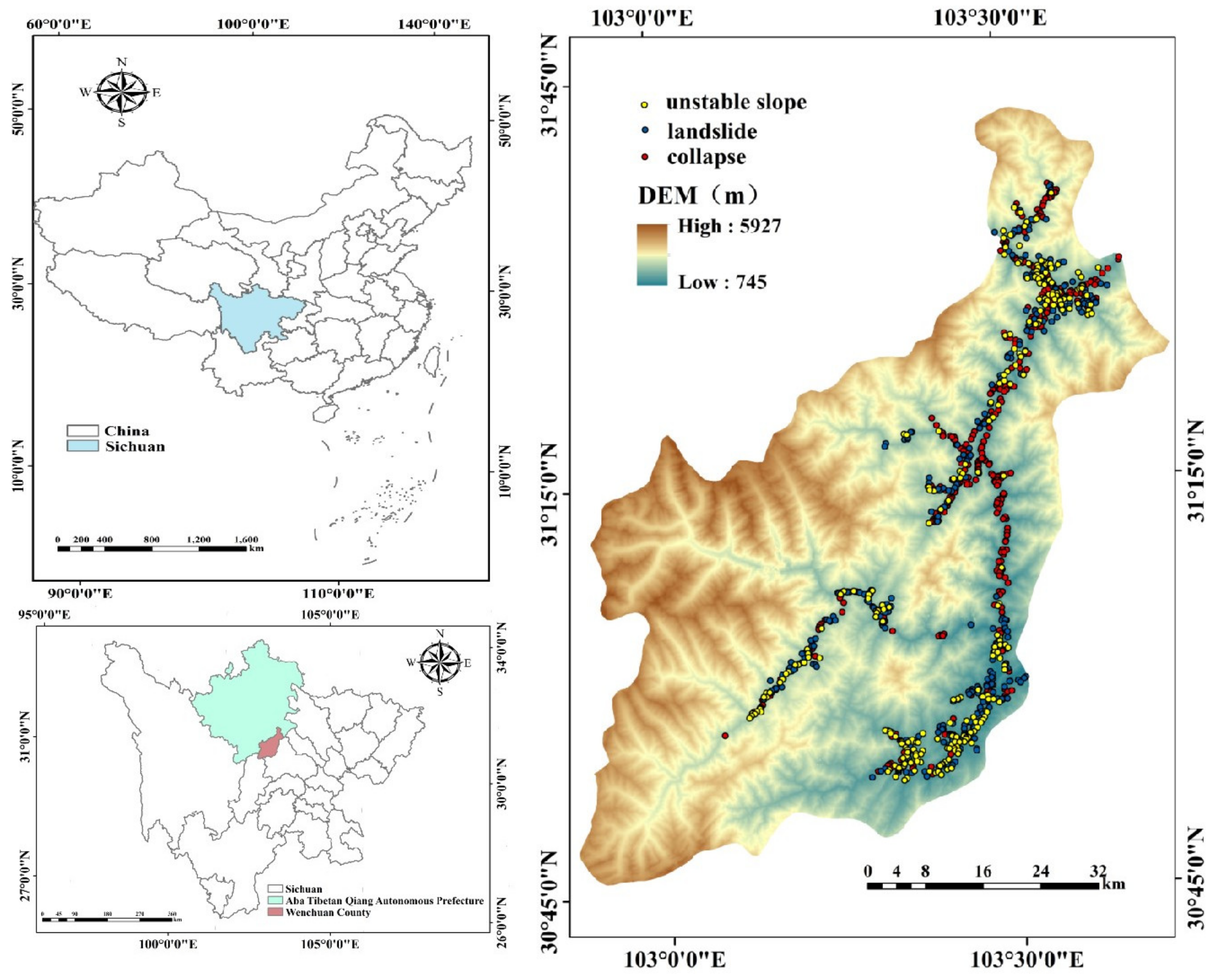
2.1. Overview of the Research Area and Collapse & Landslide Information
2.2. Data Sources
2.3. Data Description of Environmental Factors
2.4. Research Methods
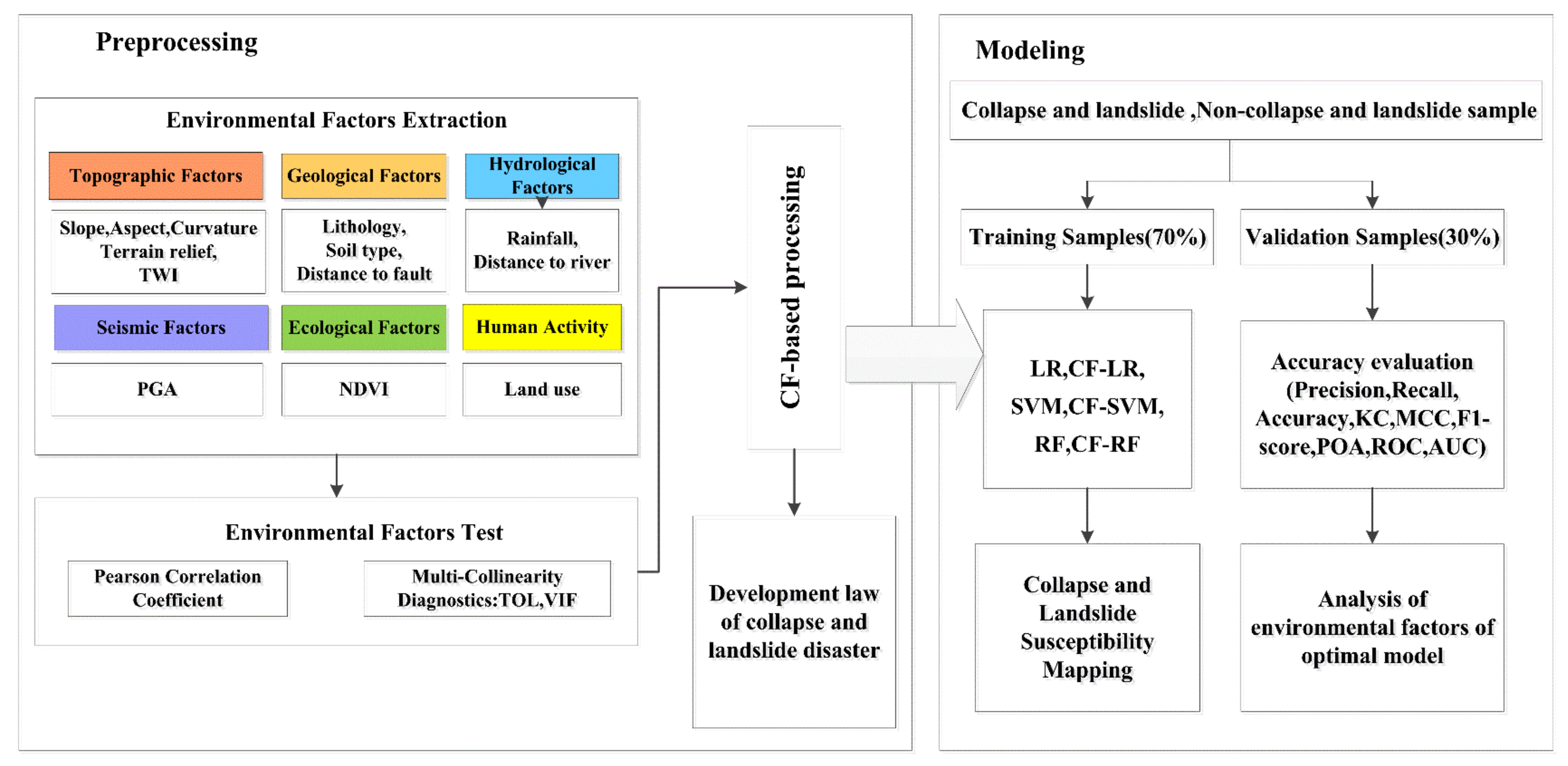
2.4.1. Research Technical Routes
2.4.2. Screening of Environmental Factors
2.4.3. Processing of the CF-Based Environmental Factors
2.4.4. Machine Learning Model
2.4.5. Performance Evaluation of the Models
3. Experimental Results
3.1. Independent Test of Environmental Factors
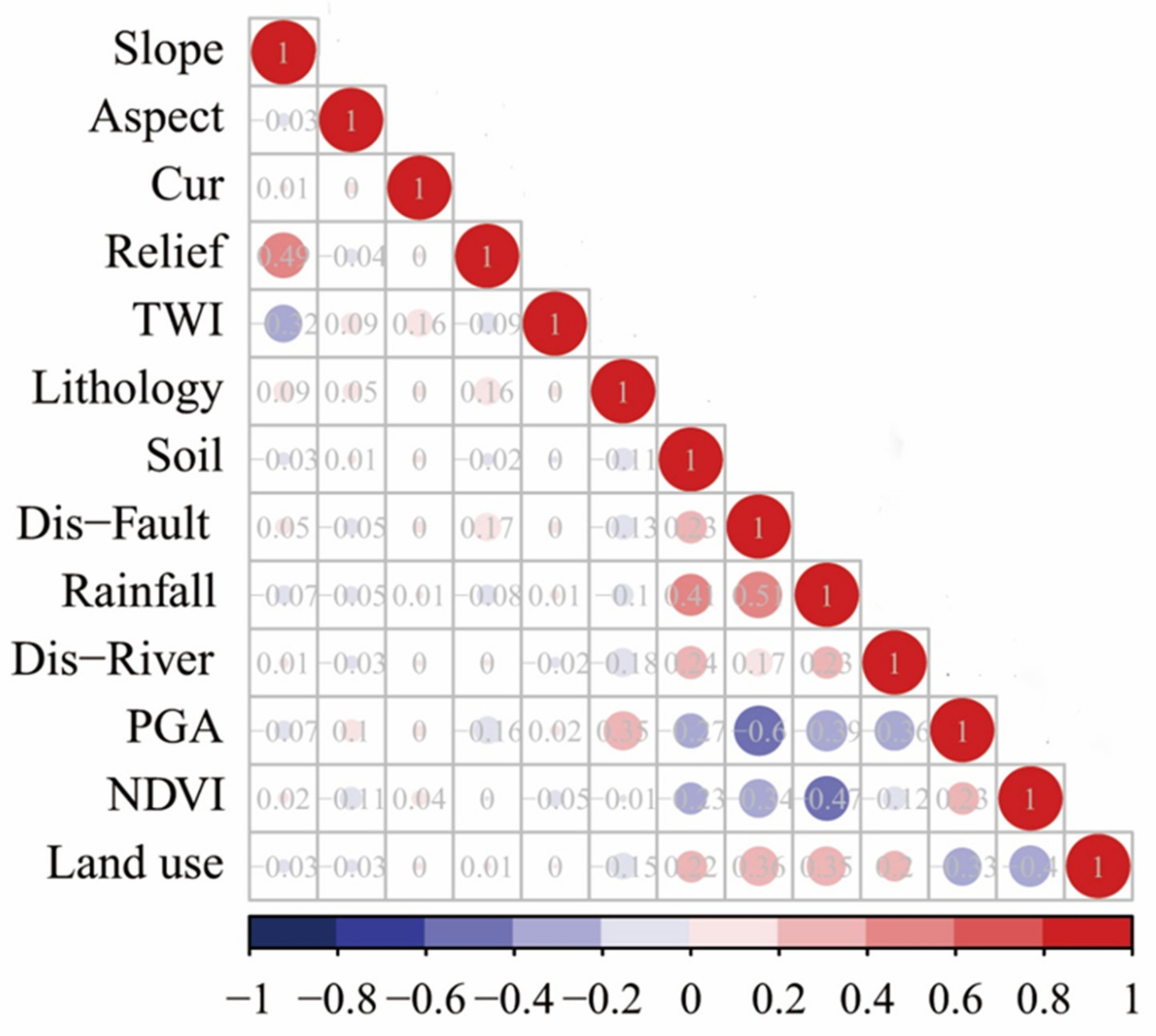
3.1.1. Correlation Analysis of the Factors
3.1.2. Multi-Collinearity Test
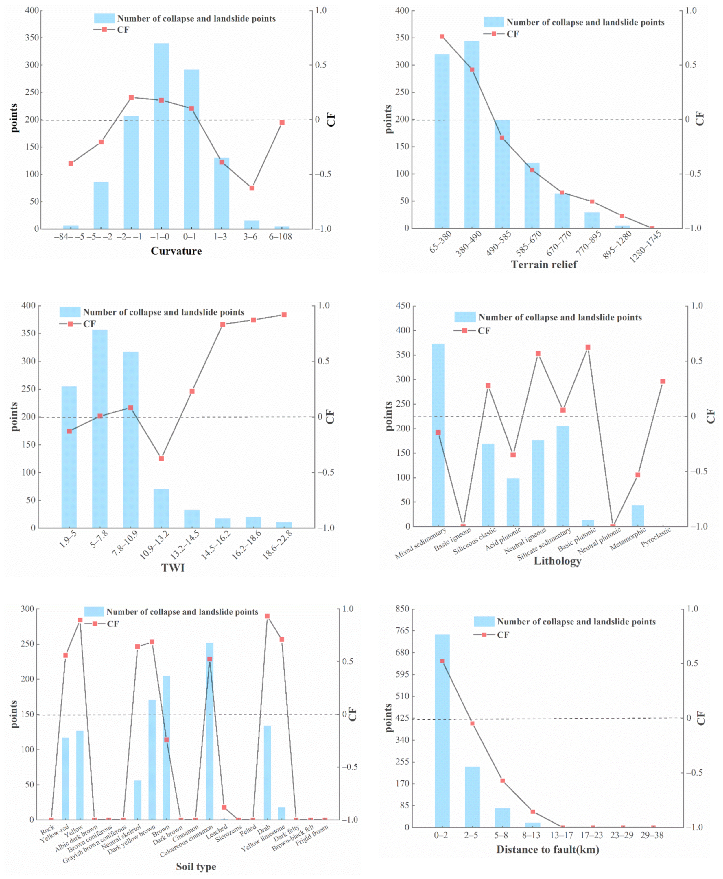
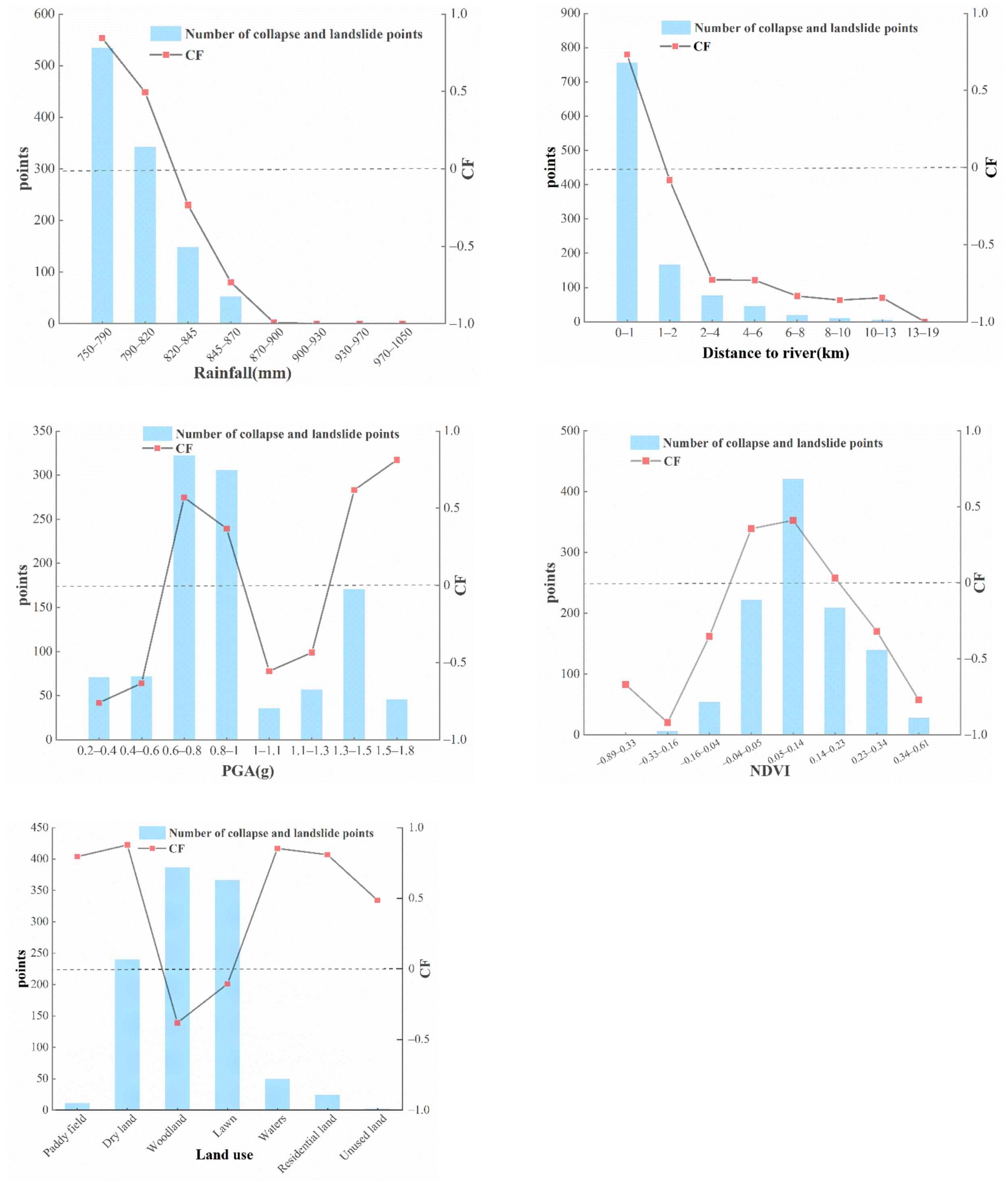
3.2. Attribute Interval Classification and Certainty Coefficient Calculation of Environmental Factors
3.3. Modeling Results
3.3.1. LR and Coupling Models
3.3.2. SVM and Coupling Models
3.3.3. RF and Coupling Models
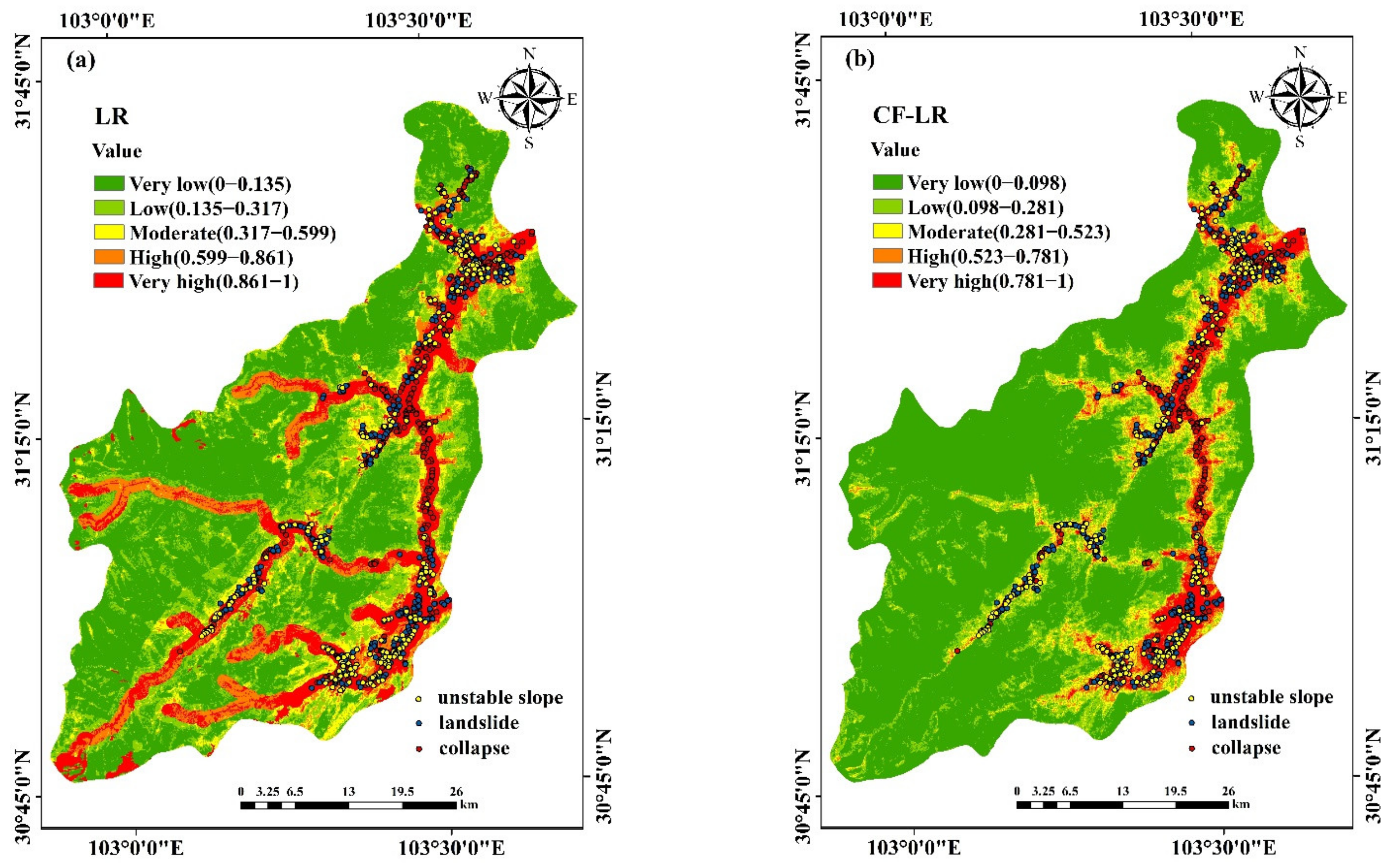
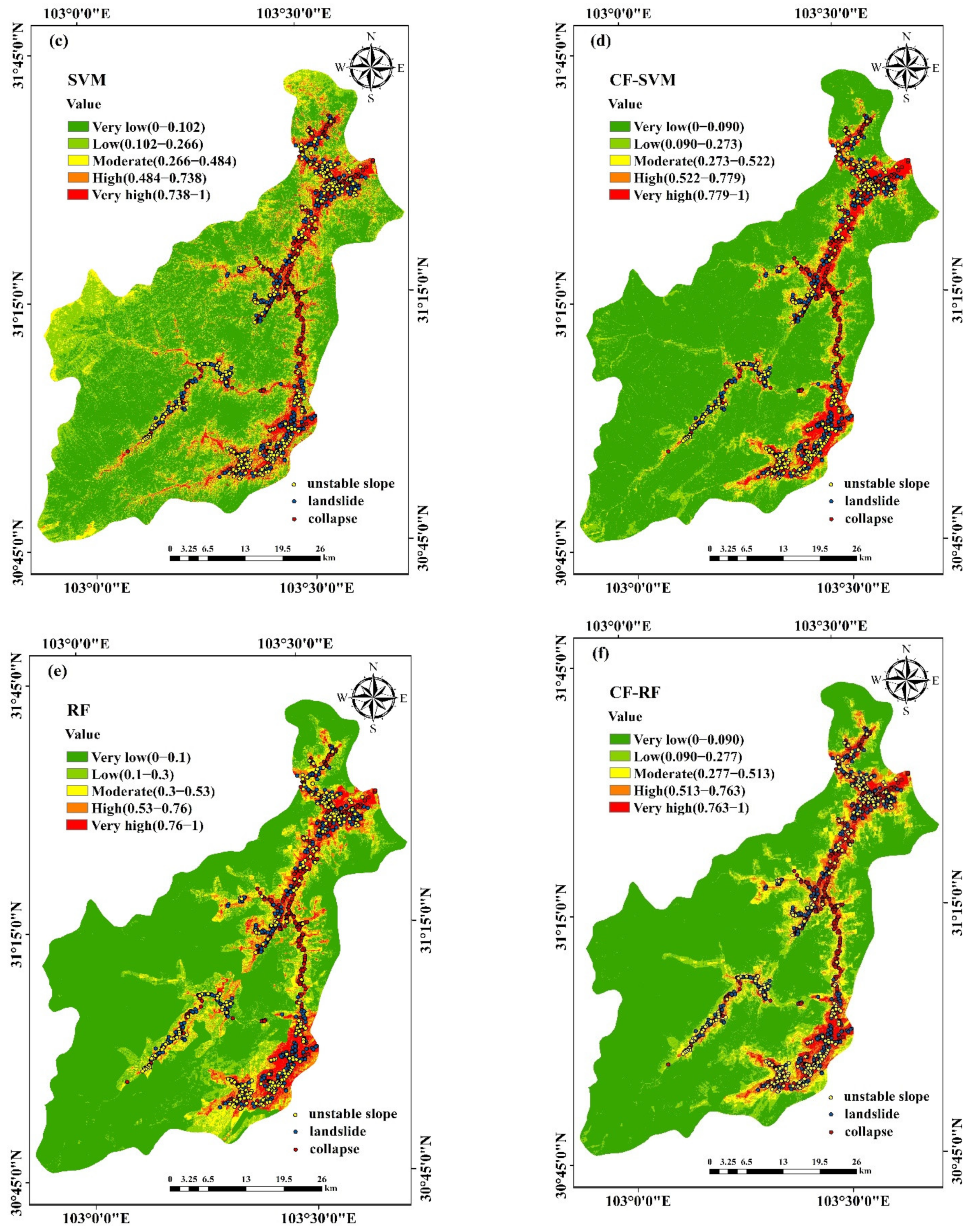
3.4. Collapse and Landslide Susceptibility Prediction Mapping
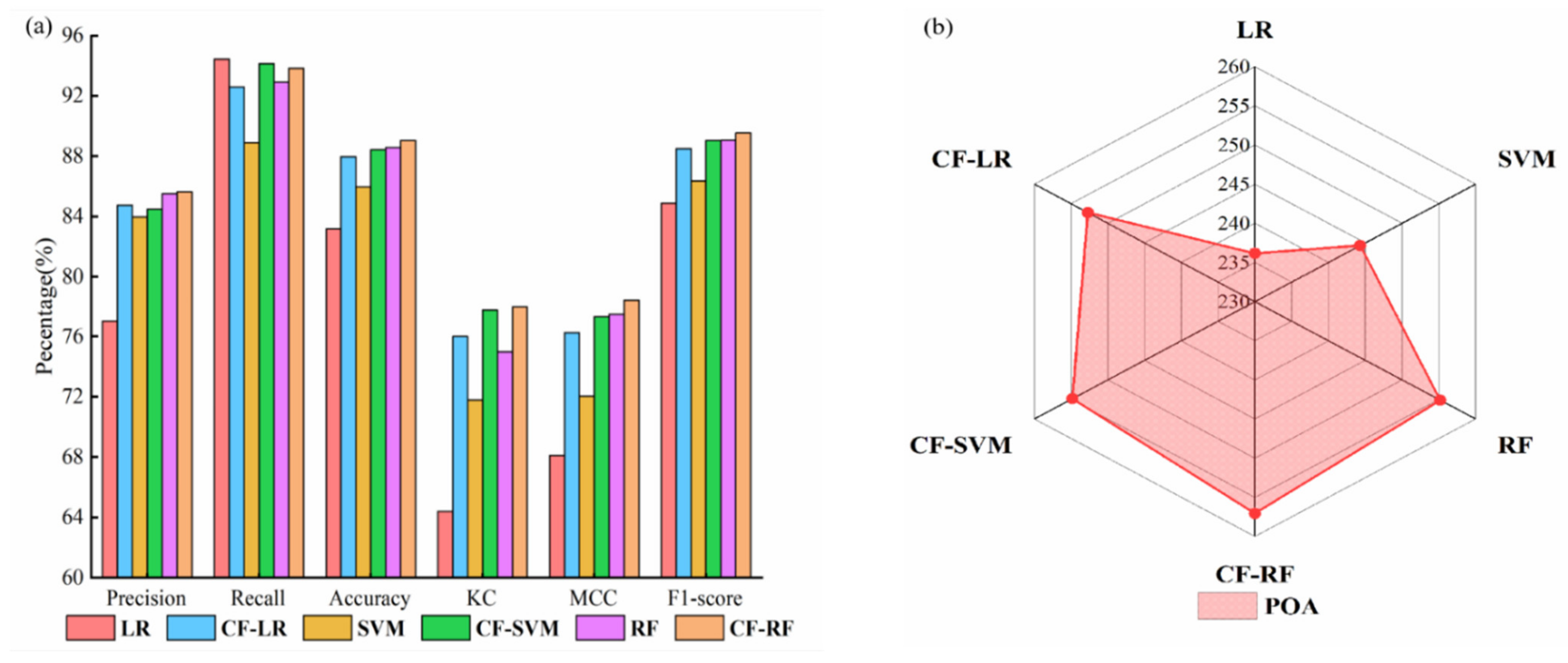
3.5. Precision Evaluation of the Models
3.5.1. Evaluation of Precision Validation Parameters
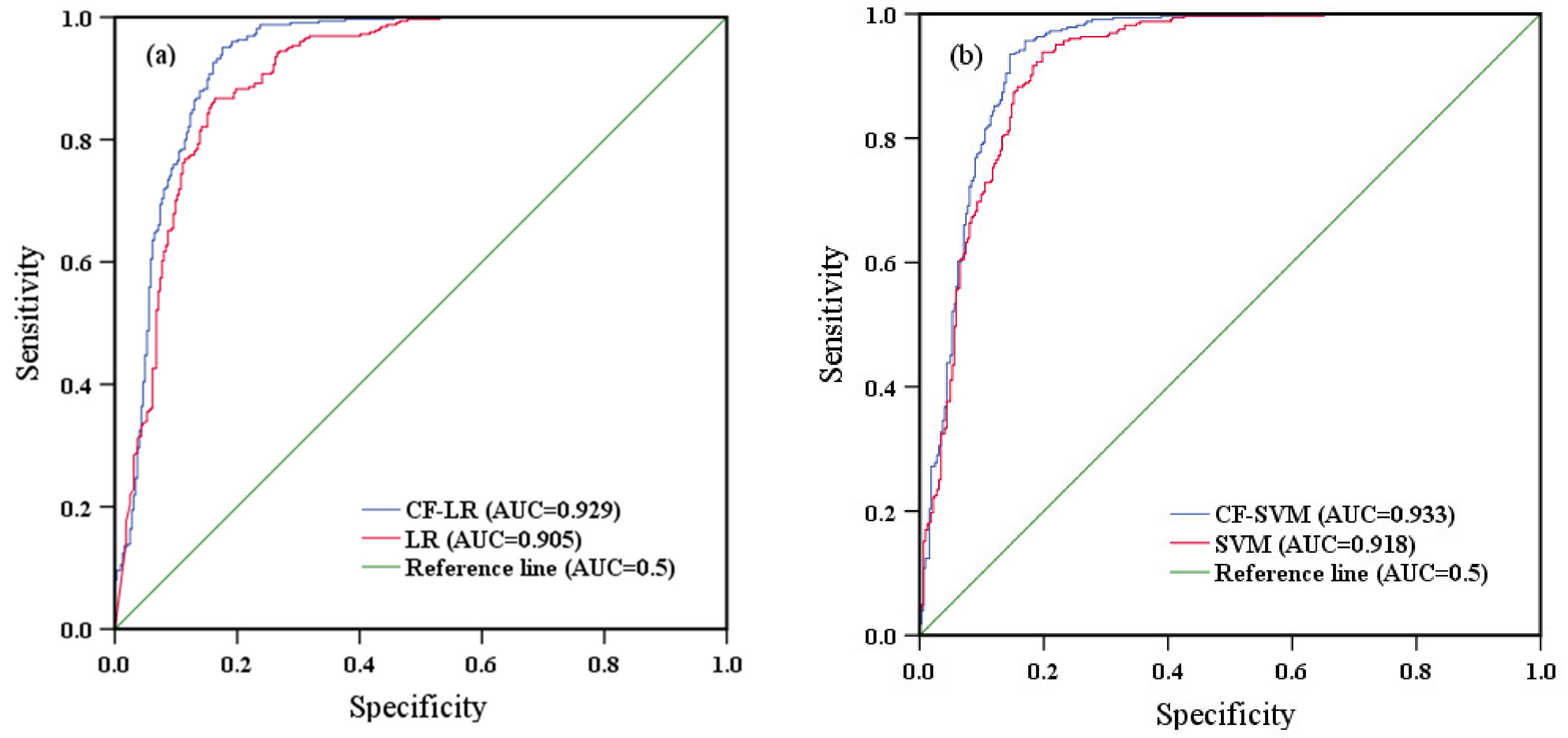
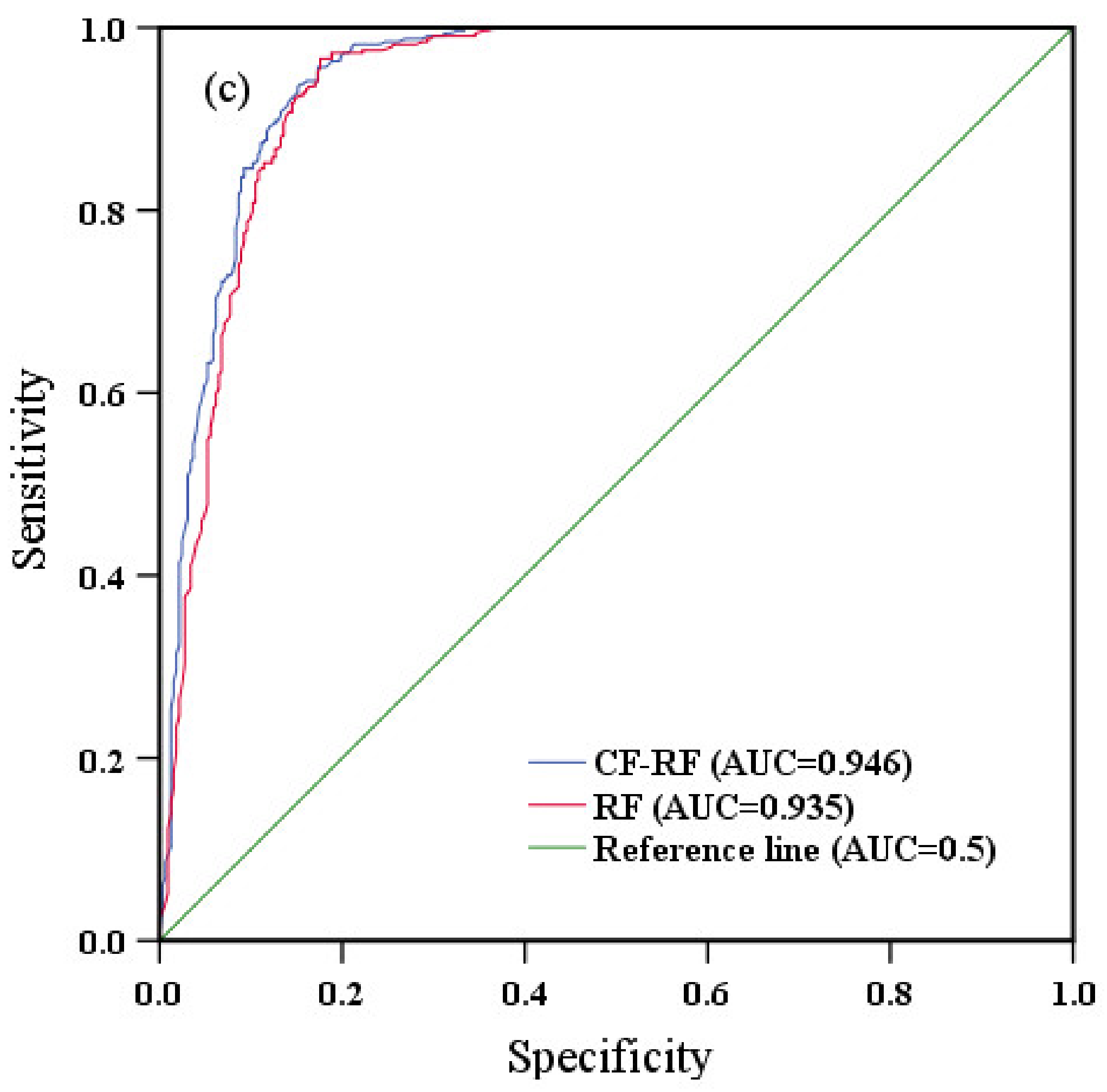
3.5.2. Comparison of ROC and AUC Results
4. Discussion
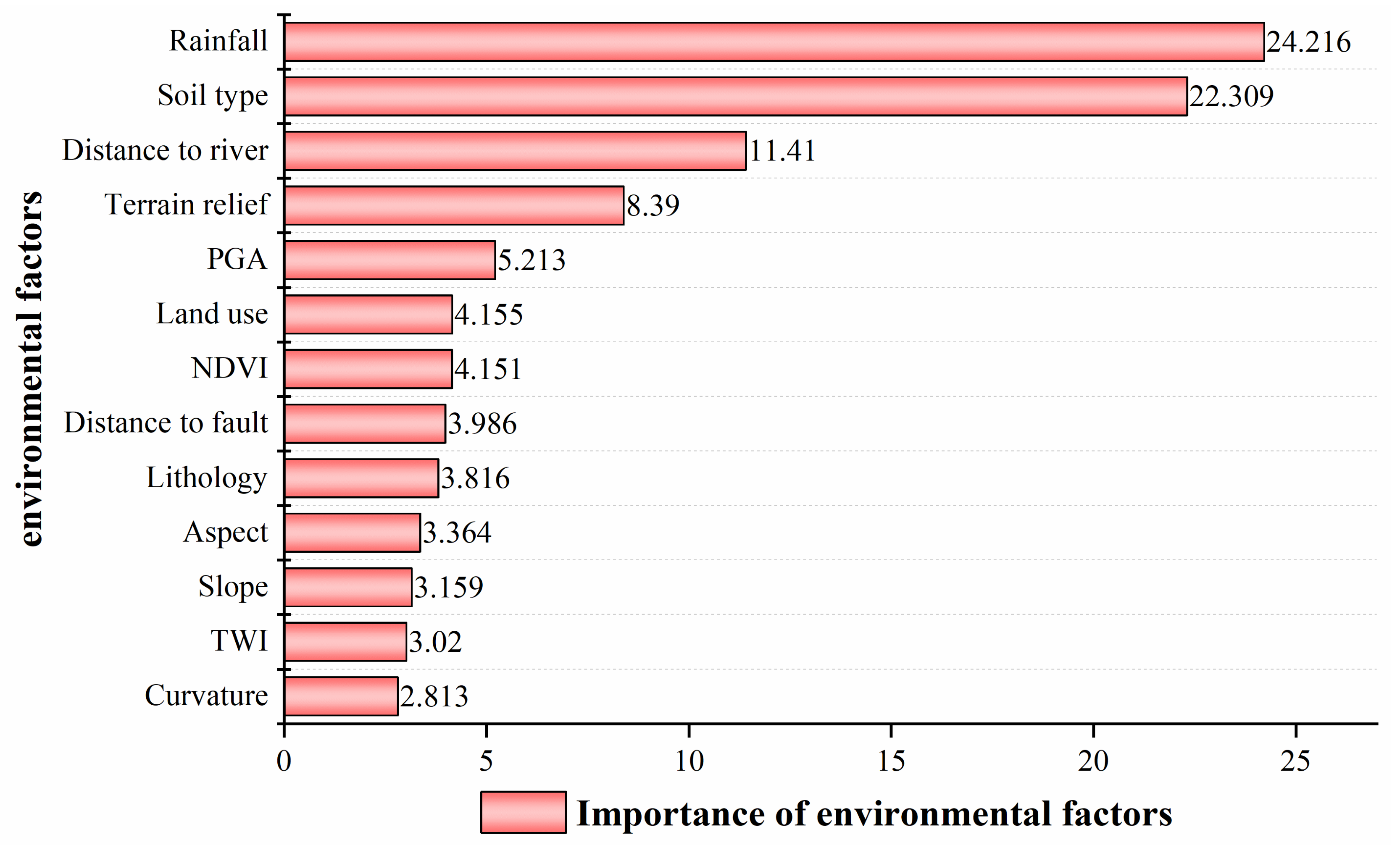
4.1. Importance Ranking of Environmental Factors
4.2. Division of Evaluation Units
4.3. Uncertainty of Hybrid Models
5. Conclusions
Author Contributions
Funding
Data Availability Statement
Conflicts of Interest
References
- Martínez-Moreno, F.J.; Galindo-Zaldívar, J.; González-Castillo, L.; Azañón, J.M. Collapse susceptibility map in abandoned mining areas by microgravity survey: A case study in Candado hill (Málaga, southern Spain). J. Appl. Geophys. 2016, 130, 101–119. [Google Scholar] [CrossRef]
- Wang, X.; Li, S.; Liu, H.; Liu, L.; Liu, Y.; Zeng, S.; Tang, Q. Landslide susceptibility assessment in Wenchuan County after the 5.12 magnitude earthquake. Bull. Eng. Geol. Environ. 2021, 80, 5369–5390. [Google Scholar] [CrossRef]
- Carrión-Mero, P.; Montalván-Burbano, N.; Morante-Carballo, F.; Quesada-Román, A.; Apolo-Masache, B. Worldwide Research Trends in Landslide Science. Int. J. Environ. Res. Public Health 2021, 18, 9445. [Google Scholar] [CrossRef] [PubMed]
- Ye, P.; Yu, B.; Chen, W.; Liu, K.; Ye, L. Rainfall-induced landslide susceptibility mapping using machine learning algorithms and comparison of their performance in Hilly area of Fujian Province, China. Nat. Hazards 2022, 1–31. [Google Scholar] [CrossRef]
- Youssef, A.M.; Pourghasemi, H.R. Landslide susceptibility mapping using machine learning algorithms and comparison of their performance at Abha Basin, Asir Region, Saudi Arabia. Di Xue Qian Yuan 2021, 12, 639–655. [Google Scholar] [CrossRef]
- Demir, G.; Aytekin, M.; Akgun, A. Landslide susceptibility mapping by frequency ratio and logistic regression methods: An example from Niksar–Resadiye (Tokat, Turkey). Arab. J. Geosci. 2015, 8, 1801–1812. [Google Scholar] [CrossRef]
- Assilzadeh, H.; Levy, J.K.; Wang, X. Landslide Catastrophes and Disaster Risk Reduction: A GIS Framework for Landslide Prevention and Management. Remote Sens. 2010, 2, 2259–2273. [Google Scholar] [CrossRef] [Green Version]
- Azarafza, M.; Ghazifard, A.; Akgün, H.; Asghari-Kaljahi, E. Landslide susceptibility assessment of South Pars Special Zone, southwest Iran. Environ. Earth Sci. 2018, 77, 805. [Google Scholar] [CrossRef]
- Thi Ngo, P.T.; Panahi, M.; Khosravi, K.; Ghorbanzadeh, O.; Kariminejad, N.; Cerda, A.; Lee, S. Evaluation of deep learning algorithms for national scale landslide susceptibility mapping of Iran. Geosci. Front. 2021, 12, 505–519. [Google Scholar] [CrossRef]
- Chen, W.; Pourghasemi, H.R.; Zhao, Z. A GIS-based comparative study of Dempster-Shafer, logistic regression and artificial neural network models for landslide susceptibility mapping. Geocarto Int. 2017, 32, 367–385. [Google Scholar] [CrossRef]
- Muñoz-Torrero Manchado, A.; Allen, S.; Ballesteros-Cánovas, J.A.; Dhakal, A.; Dhital, M.R.; Stoffel, M. Three decades of landslide activity in western Nepal: New insights into trends and climate drivers. Landslides 2021, 18, 2001–2015. [Google Scholar] [CrossRef]
- Quesada-Román, A. Landslide risk index map at the municipal scale for Costa Rica. Int. J. Disaster Risk Reduct. 2021, 56, 102144. [Google Scholar] [CrossRef]
- Ali, S.A.; Parvin, F.; Vojteková, J.; Costache, R.; Linh, N.T.T.; Pham, Q.B.; Vojtek, M.; Gigović, L.; Ahmad, A.; Ghorbani, M.A. GIS-based landslide susceptibility modeling: A comparison between fuzzy multi-criteria and machine learning algorithms. Geosci. Front. 2021, 12, 857–876. [Google Scholar] [CrossRef]
- Quesada-Román, A.; Fallas-López, B.; Hernández-Espinoza, K.; Stoffel, M.; Ballesteros-Cánovas, J.A. Relationships between earthquakes, hurricanes, and landslides in Costa Rica. Landslides 2019, 16, 1539–1550. [Google Scholar] [CrossRef]
- Bahrami, Y.; Hassani, H.; Maghsoudi, A. Landslide susceptibility mapping using AHP and fuzzy methods in the Gilan province, Iran. GeoJournal 2021, 86, 1797–1816. [Google Scholar] [CrossRef]
- Tao, Y.; Xue, Y.; Zhang, Q.; Yang, W.; Li, B.; Zhang, L.; Qu, C.; Zhang, K. Risk Assessment of Unstable Rock Masses on High-Steep Slopes: An Attribute Recognition Model. Soil Mech. Found. Eng. 2021, 58, 175–182. [Google Scholar] [CrossRef]
- Zhao, X.; Chen, W. Optimization of Computational Intelligence Models for Landslide Susceptibility Evaluation. Remote Sens. 2020, 12, 2180. [Google Scholar] [CrossRef]
- Chen, W.; Li, H.; Hou, E.; Wang, S.; Wang, G.; Panahi, M.; Li, T.; Peng, T.; Guo, C.; Niu, C.; et al. GIS-based groundwater potential analysis using novel ensemble weights-of-evidence with logistic regression and functional tree models. Sci. Total Environ. 2018, 634, 853–867. [Google Scholar] [CrossRef] [Green Version]
- Hong, H.; Chen, W.; Xu, C.; Youssef, A.M.; Pradhan, B.; Tien Bui, D. Rainfall-induced landslide susceptibility assessment at the Chongren area (China) using frequency ratio, certainty factor, and index of entropy. Geocarto Int. 2017, 32, 139–154. [Google Scholar] [CrossRef]
- Aditian, A.; Kubota, T.; Shinohara, Y. Comparison of GIS-based landslide susceptibility models using frequency ratio, logistic regression, and artificial neural network in a tertiary region of Ambon, Indonesia. Geomorphology 2018, 318, 101–111. [Google Scholar] [CrossRef]
- Polat, A. An innovative, fast method for landslide susceptibility mapping using GIS-based LSAT toolbox. Environ. Earth Sci. 2021, 80, 217. [Google Scholar] [CrossRef]
- Zheng, H.; Liu, B.; Han, S.; Fan, X.; Zou, T.; Zhou, Z.; Gong, H. Research on landslide hazard spatial prediction models based on deep neural networks: A case study of northwest Sichuan, China. Environ. Earth Sci. 2022, 81, 258. [Google Scholar] [CrossRef]
- Zêzere, J.L.; Pereira, S.; Melo, R.; Oliveira, S.C.; Garcia, R.A.C. Mapping landslide susceptibility using data-driven methods. Sci. Total Environ. 2017, 589, 250–267. [Google Scholar] [CrossRef]
- Sun, D.; Wen, H.; Wang, D.; Xu, J. A random forest model of landslide susceptibility mapping based on hyperparameter optimization using Bayes algorithm. Geomorphology 2020, 362, 107201. [Google Scholar] [CrossRef]
- Arabameri, A.; Chen, W.; Loche, M.; Zhao, X.; Li, Y.; Lombardo, L.; Cerda, A.; Pradhan, B.; Bui, D.T. Comparison of machine learning models for gully erosion susceptibility mapping. Geosci. Front. 2020, 11, 1609–1620. [Google Scholar] [CrossRef]
- Lin, J.; He, P.; Yang, L.; He, X.; Lu, S.; Liu, D. Predicting future urban waterlogging-prone areas by coupling the maximum entropy and FLUS model. Sustain. Cities Soc. 2022, 80, 103812. [Google Scholar] [CrossRef]
- Javidan, N.; Kavian, A.; Pourghasemi, H.R.; Conoscenti, C.; Jafarian, Z.; Rodrigo-Comino, J. Evaluation of multi-hazard map produced using MaxEnt machine learning technique. Sci. Rep. 2021, 11, 6496. [Google Scholar] [CrossRef]
- Rahmati, O.; Golkarian, A.; Biggs, T.; Keesstra, S.; Mohammadi, F.; Daliakopoulos, I.N. Land subsidence hazard modeling: Machine learning to identify predictors and the role of human activities. J. Environ. Manag. 2019, 236, 466–480. [Google Scholar] [CrossRef]
- Zhang, S.; Bai, L.; Li, Y.; Li, W.; Xie, M. Comparing Convolutional Neural Network and Machine Learning Models in Landslide Susceptibility Mapping: A Case Study in Wenchuan County. Front. Environ. Sci. 2022, 10, 496. [Google Scholar] [CrossRef]
- Chen, W.; Peng, J.; Hong, H.; Shahabi, H.; Pradhan, B.; Liu, J.; Zhu, A.; Pei, X.; Duan, Z. Landslide susceptibility modelling using GIS-based machine learning techniques for Chongren County, Jiangxi Province, China. Sci. Total Environ. 2018, 626, 1121–1135. [Google Scholar] [CrossRef]
- Chen, W.; Li, Y. GIS-based evaluation of landslide susceptibility using hybrid computational intelligence models. Catena 2020, 195, 104777. [Google Scholar] [CrossRef]
- Trinh, T.; Luu, B.T.; Le, T.H.T.; Nguyen, D.H.; Van Tran, T.; Van Nguyen, T.H.; Nguyen, K.Q.; Nguyen, L.T. A comparative analysis of weight-based machine learning methods for landslide susceptibility mapping in Ha Giang area. Big Earth Data 2022, 1–30, ahead of print. [Google Scholar] [CrossRef]
- Zhou, X.; Wu, W.; Qin, Y.; Fu, X. Geoinformation-based landslide susceptibility mapping in subtropical area. Sci. Rep. 2021, 11, 24325. [Google Scholar] [CrossRef] [PubMed]
- Qiu, C.; Su, L.; Zou, Q.; Geng, X. A hybrid machine-learning model to map glacier-related debris flow susceptibility along Gyirong Zangbo watershed under the changing climate. Sci. Total Environ. 2022, 818, 151752. [Google Scholar] [CrossRef]
- Xu, C.; Xu, X.; Zhou, B.; Yu, G. Revisions of the M 8.0 Wenchuan earthquake seismic intensity map based on co-seismic landslide abundance. Nat. Hazards 2013, 69, 1459–1476. [Google Scholar] [CrossRef]
- Zhu, J.; Ding, J.; Liang, J. Influences of the Wenchuan Earthquake on sediment supply of debris flows. J. Mt. Sci. 2011, 8, 270–277. [Google Scholar] [CrossRef]
- Huang, R.; Li, W. Post-earthquake landsliding and long-term impacts in the Wenchuan earthquake area, China. Eng. Geol. 2014, 182, 111–120. [Google Scholar] [CrossRef]
- Evik, E.; Topal, T. GIS-based landslide susceptibility mapping for a problematic segment of the natural gas pipeline, Hendek (Turkey). Environ. Geol. 2003, 44, 949–962. [Google Scholar]
- Gnyawali, K.R.; Zhang, Y.; Wang, G.; Miao, L.; Pradhan, A.M.S.; Adhikari, B.R.; Xiao, L. Mapping the susceptibility of rainfall and earthquake triggered landslides along China–Nepal highways. Bull. Eng. Geol. Environ. 2020, 79, 587–601. [Google Scholar] [CrossRef]
- Mersha, T.; Meten, M. GIS-based landslide susceptibility mapping and assessment using bivariate statistical methods in Simada area, northwestern Ethiopia. Geoenviron. Disasters 2020, 7, 20. [Google Scholar] [CrossRef]
- Sajinkumar, K.S.; Anbazhagan, S. Geomorphic appraisal of landslides on the windward slope of Western Ghats, southern India. Nat. Hazards 2015, 75, 953–973. [Google Scholar] [CrossRef]
- Beven, K.J.; Kirkby, M.J.; Schofield, N.; Tagg, A.F. Testing a physically-based flood forecasting model (TOPMODEL) for three U.K. catchments. J. Hydrol. 1984, 69, 119–143. [Google Scholar] [CrossRef]
- Pachuau, L. Zonation of Landslide Susceptibility and Risk Assessment in Serchhip town, Mizoram. J. Indian Soc. Remote 2019, 47, 1587–1597. [Google Scholar] [CrossRef]
- Bucci, F.; Santangelo, M.; Cardinali, M.; Fiorucci, F.; Guzzetti, F. Landslide distribution and size in response to Quaternary fault activity: The Peloritani Range, NE Sicily, Italy. Earth Surf. Proc. Land. 2016, 41, 711–720. [Google Scholar] [CrossRef] [Green Version]
- Steger, S.; Brenning, A.; Bell, R.; Petschko, H.; Glade, T. Exploring discrepancies between quantitative validation results and the geomorphic plausibility of statistical landslide susceptibility maps. Geomorphology 2016, 262, 8–23. [Google Scholar] [CrossRef]
- Yi, Y.; Zhang, Z.; Zhang, W.; Xu, Q.; Deng, C.; Li, Q. GIS-based earthquake-triggered-landslide susceptibility mapping with an integrated weighted index model in Jiuzhaigou region of Sichuan Province, China. Nat. Hazard. Earth Sys. 2019, 19, 1973–1988. [Google Scholar] [CrossRef] [Green Version]
- Peduzzi, P. Landslides and vegetation cover in the 2005 north Pakistan earthquake; a GIS and statistical quantitative approach. Nat. Hazard. Earth Sys. 2010, 10, 623–640. [Google Scholar] [CrossRef]
- Pham, V.D.; Nguyen, Q.; Nguyen, H.; Pham, V.; Vu, V.M.; Bui, Q. Convolutional Neural Network—Optimized Moth Flame Algorithm for Shallow Landslide Susceptible Analysis. IEEE Access 2020, 8, 32727–32736. [Google Scholar] [CrossRef]
- Cheng, J.; Dai, X.; Wang, Z.; Li, J.; Qu, G.; Li, W.; She, J.; Wang, Y. Landslide Susceptibility Assessment Model Construction Using Typical Machine Learning for the Three Gorges Reservoir Area in China. Remote Sens. 2022, 14, 2257. [Google Scholar] [CrossRef]
- Shahzad, N.; Ding, X.; Abbas, S. A Comparative Assessment of Machine Learning Models for Landslide Susceptibility Mapping in the Rugged Terrain of Northern Pakistan. Appl. Sci. 2022, 12, 2280. [Google Scholar] [CrossRef]
- Shortliffe, E.H. A Model of Inexact Reasoning in Medicine. Math. Biosci. 1975, 23, 351–379. [Google Scholar] [CrossRef]
- Heckerman, D.E.; Shortliffe, E.H. From certainty factors to belief networks. Artif. Intell. Med. 1992, 4, 35–52. [Google Scholar] [CrossRef]
- Chen, W.; Li, W.; Chai, H.; Hou, E.; Li, X.; Ding, X. GIS-based landslide susceptibility mapping using analytical hierarchy process (AHP) and certainty factor (CF) models for the Baozhong region of Baoji City, China. Environ. Earth Sci. 2016, 75, 63. [Google Scholar] [CrossRef]
- Dou, J.; Tien Bui, D.; Yunus, A.P.; Jia, K.; Song, X.; Revhaug, I.; Xia, H.; Zhu, Z. Optimization of Causative Factors for Landslide Susceptibility Evaluation Using Remote Sensing and GIS Data in Parts of Niigata, Japan. PLoS ONE 2015, 10, e133262. [Google Scholar] [CrossRef] [Green Version]
- Paryani, S.; Neshat, A.; Javadi, S.; Pradhan, B. Comparative performance of new hybrid ANFIS models in landslide susceptibility mapping. Nat. Hazards 2020, 103, 1961–1988. [Google Scholar] [CrossRef]
- Dou, J.; Yamagishi, H.; Pourghasemi, H.R.; Yunus, A.P.; Song, X.; Xu, Y.; Zhu, Z. An integrated artificial neural network model for the landslide susceptibility assessment of Osado Island, Japan. Nat. Hazards 2015, 78, 1749–1776. [Google Scholar] [CrossRef]
- Vapnik, V.N. The support vector method. In Proceedings of the 7th International Conference on Artificial Neural Networks, Lausanne, Switzerland, 8–10 October 1997; pp. 263–271. [Google Scholar]
- Cortes, C.; Vapnik, V. Cortes-Vapnik1995_Article_Support-vectorNetworks. Support-vector networks. Mach. Learn. 1995, 20, 273–297. [Google Scholar] [CrossRef]
- Breiman, L. Breiman2001_Article_RandomForests. Random Forests. Mach. Learn. 2001, 45, 5–32. [Google Scholar] [CrossRef] [Green Version]
- Wang, H.; Zhang, L.; Yin, K.; Luo, H.; Li, J. Landslide identification using machine learning. Geosci. Front. 2021, 12, 351–364. [Google Scholar] [CrossRef]
- Zhou, X.; Wu, W.; Lin, Z.; Zhang, G.; Chen, R.; Song, Y.; Wang, Z.; Lang, T.; Qin, Y.; Ou, P.; et al. Zonation of Landslide Susceptibility in Ruijin, Jiangxi, China. Int. J. Environ. Res. Public Health 2021, 18, 5906. [Google Scholar] [CrossRef]
- Kreuzer, T.M.; Wilde, M.; Terhorst, B.; Damm, B. A landslide inventory system as a base for automated process and risk analyses. Earth Sci. Inform. 2017, 10, 507–515. [Google Scholar] [CrossRef] [Green Version]
- Zhang, T.; Fu, Q.; Quevedo, R.P.; Chen, T.; Luo, D.; Liu, F.; Kong, H. Landslide Susceptibility Mapping Using Novel Hybrid Model Based on Different Mapping Units. KSCE J. Civ. Eng. 2022, 26, 2888–2900. [Google Scholar] [CrossRef]
- Ba, Q.; Chen, Y.; Deng, S.; Yang, J.; Li, H. A comparison of slope units and grid cells as mapping units for landslide susceptibility assessment. Earth Sci. Inform. 2018, 11, 373–388. [Google Scholar] [CrossRef]
- Liu, X.; Su, P.; Li, Y.; Zhang, J.; Yang, T. Susceptibility assessment of small, shallow and clustered landslide. Earth Sci. Inform. 2021, 14, 2347–2356. [Google Scholar] [CrossRef]
- Wang, F.; Xu, P.; Wang, C.; Wang, N.; Jiang, N. Application of a GIS-Based Slope Unit Method for Landslide Susceptibility Mapping along the Longzi River, Southeastern Tibetan Plateau, China. ISPRS Int. J. Geo.-Inf. 2017, 6, 172. [Google Scholar] [CrossRef] [Green Version]
- Qin, Y.; Yang, G.; Lu, K.; Sun, Q.; Xie, J.; Wu, Y. Performance Evaluation of Five GIS-Based Models for Landslide Susceptibility Prediction and Mapping: A Case Study of Kaiyang County, China. Sustainability 2021, 13, 6441. [Google Scholar] [CrossRef]
- Zhao, B.; Ge, Y.; Chen, H. Landslide susceptibility assessment for a transmission line in Gansu Province, China by using a hybrid approach of fractal theory, information value, and random forest models. Environ. Earth Sci. 2021, 80, 441. [Google Scholar] [CrossRef]
- Xiao, T.; Yin, K.; Yao, T.; Liu, S. Spatial prediction of landslide susceptibility using GIS-based statistical and machine learning models in Wanzhou County, Three Gorges Reservoir, China. Acta Geochim. 2019, 38, 654–669. [Google Scholar] [CrossRef]
- Mohajane, M.; Costache, R.; Karimi, F.; Bao Pham, Q.; Essahlaoui, A.; Nguyen, H.; Laneve, G.; Oudija, F. Application of remote sensing and machine learning algorithms for forest fire mapping in a Mediterranean area. Ecol. Indic. 2021, 129, 107869. [Google Scholar] [CrossRef]


| Data Type | Data Sources | Usage | Spatial Resolution |
|---|---|---|---|
| The distribution data of geological disaster points | Sichuan Geological Survey | Divide the training set and the validation set | Vector data |
| The digital elevation model (DEM) | NASA official website (https://search.asf.alaska.edu/#/) | Obtain slope, aspect, curvature, terrain relief, and topographic wetness index | 30 m × 30 m |
| The river data | The thematic map of the river system in China from 91 satellite map assistant software | Obtain the distance to river | 1:500,000 |
| The fault data | Geological map from 91 satellite map assistant software | Obtain the distance to fault | 1:500,000 |
| The rainfall data | The Resource and Environment Science and Data Center of Chinese Academy of Sciences (http://www.resdc.cn/) | Obtain average annual rainfall | 1000 m × 1000 m |
| The Landsat 8 OLI image on 9 April 2018 | The geospatial data cloud network (http://www.gscloud.cn/) | Obtain the normalized difference vegetation index | 30 m × 30 m |
| The lithology data | Sichuan Geological Survey | Obtain the lithology | 30 m × 30 m |
| The soil data | The geospatial data cloud network (http://www.gscloud.cn/) | Obtain the soil | 30 m × 30 m |
| Land use | Geospatial data cloud (http://www.gscloud.cn/) | Obtain the data of land use | 30 m × 30 m |
| The seismic peak ground acceleration | The United States Geological Survey (USGS) (https://earthquake.usgs.gov/) | Obtain seismic peak ground acceleration | Vector data |
| Data Type | Factors | Reason for Selecting the Parameters |
|---|---|---|
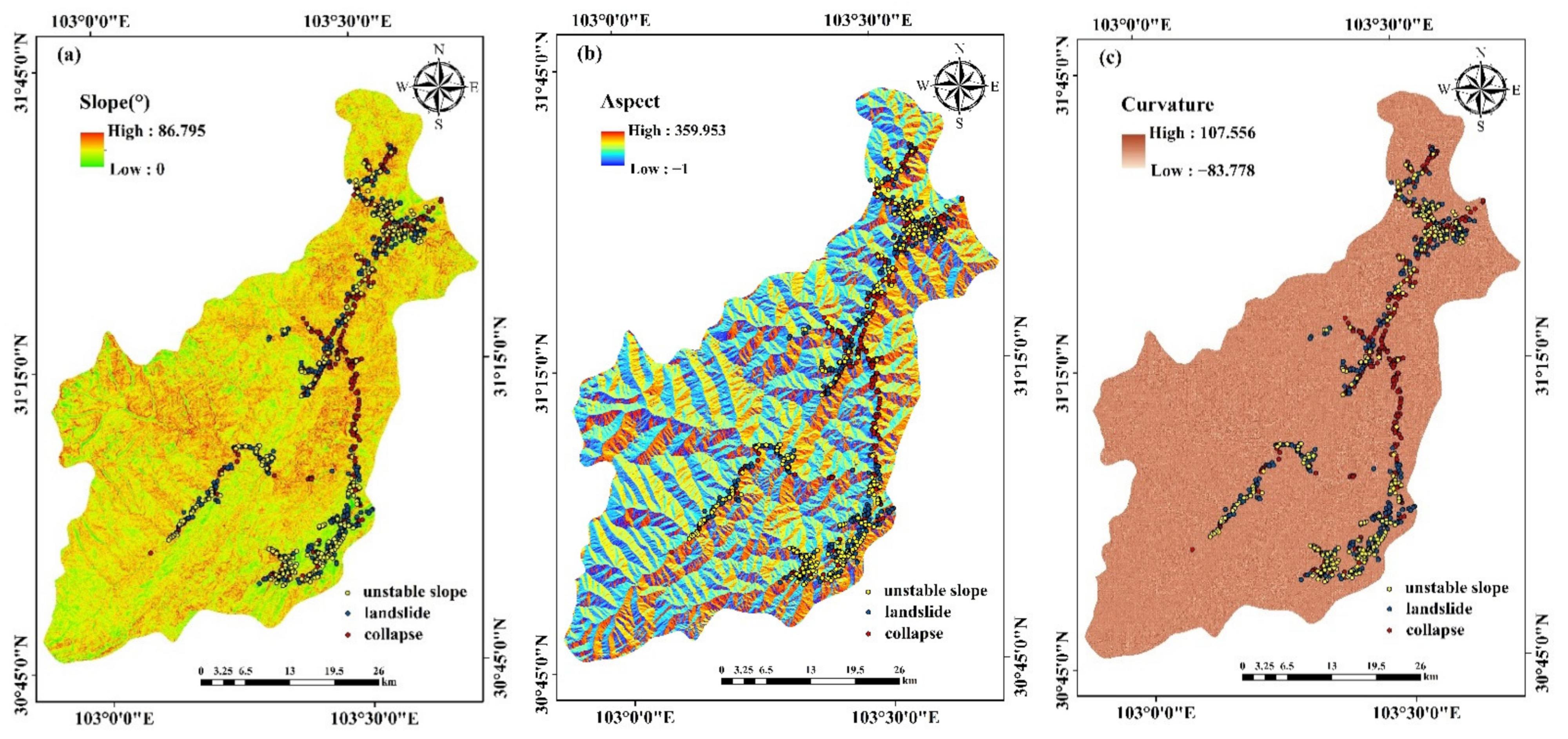
| Topographic | Slope | Slope affects water flow direction and soil development, which is one of the important reasons for slope instability [20]. The more the slope increases, the more concentrated the shear stress in the slope is, and the greater the possibility of occurrence of collapse and landslide disasters will be [23]. |
| Aspect | The influence of aspect on collapse and landslide is the regular difference of microclimate and water heat ratio of hillside. The sunshine duration, solar radiation intensity, and daily temperature difference are different on slopes with different aspects [38]. | |
| Curvature | Curvature is defined as the change rate of the slope and the shape of the earth’s surface, which has a great impact on the transportation of collapse and landslide materials [39]. The greater the concave–convex degree of the slope is, the more unstable the slope is, and the more likely it is that collapse and landslide will occur [40]. Negative curvature, zero curvature, and positive curvature represent concave surfaces, plane surfaces, and convex surfaces, respectively. | |
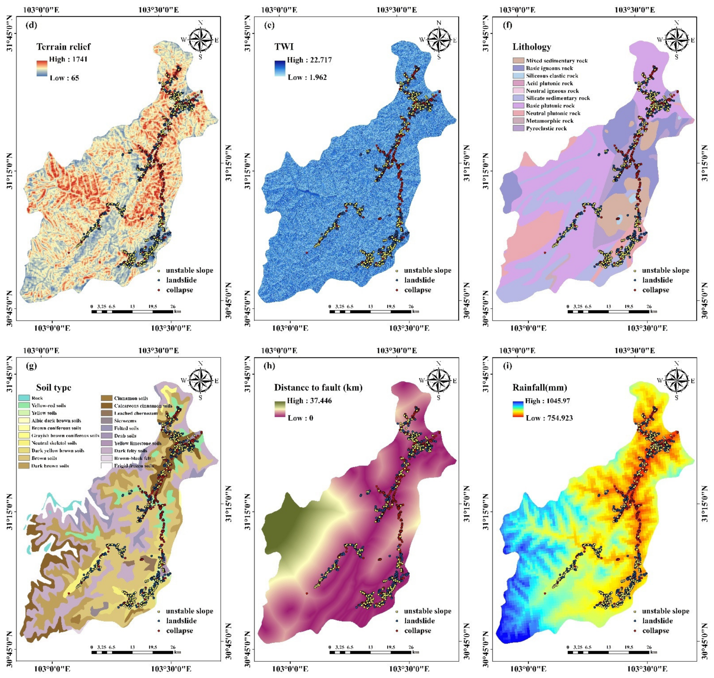
| Terrain relief | The terrain relief reflects the difference between the highest point and the lowest point of altitude in a specific area, and controls the gravitational potential energy that can cause collapse and landslide disasters [41]. The greater the terrain relief is, the more fractured the terrain is, the higher the instability of the surface soil layer and slope is, and the more likely it is that collapse and landslide disasters will occur. | |
| Topographic wetness index (TWI) | The topographic wetness index refers to the influence of the scale and terrain of the saturated runoff zone on the region, and is used to quantify the control of terrain on hydrological processes. By comprehensively considering the impact of terrain and soil characteristics on soil moisture distribution, Beven and Kirkby proposed [42] the calculation formula , where represents the drainage area and represents the slope angle. | |
| Geological | Lithology | The rock-soil type and structural characteristics control the stress distribution, strength, and deformation and failure characteristics [43] of the rock-soil mass of the slope. Slopes with different lithology have different shear strength and stability, and also have different probability of occurrence of collapse and landslide disasters. |
| Soil type | Different soil types have different shear strength and hydraulic conductivity, which affect the stability of slopes [31]. | |
| Distance to fault | The rock mass is broken, the rock has poor erosion and weathering resistance, and the slope has poor stability near the fault zone [44]. | |
| Hydrological | Rainfall | Rainfall infiltration not only softens the rock-soil mass of the slope, but also increases the seepage pressure. The formed surface runoff will scour and erode the slope, resulting in the instability of the slope. The average annual rainfall affects the slope and its ecological environment, thus affecting the occurrence of collapse and landslide disasters [24]. |
| Distance to river | The softening, scouring, and erosion caused by river erosion have a serious impact on the stability of the slope. Slopes located in the coastal area of a river are eroded by the river and infiltrated by water, which leads to changes in internal stress and a greater probability of occurrence of collapses and landslides [45]. | |
| Seismic | Peak ground acceleration (PGA) | As an important dynamic factor to measure the impact of earthquakes on collapse and landslide, seismic peak ground acceleration reflects the overall vibration intensity of the earth’s surface after an earthquake. The intense activity of the earth’s surface reduces the stability of the rock-soil mass and increases the possibility of occurrence of collapse and landslide disasters [46]. |
| Ecological | Normalized difference vegetation index (NDVI) | As an important index that can reflect the growth status and coverage of vegetation, NDVI can inhibit the occurrence of collapses and landslides to a certain extent [47]. The calculation formula is , where represents the reflectance in near-infrared wavelength and represents the reflectance in red light wavelength. |
| Human activity | Land use | The type of land use not only affects soil moisture and surface runoff, but also indirectly affects the development of landslides and collapses [48]. |
| Prediction Situation | Actual Situation | |
|---|---|---|
| Positive Sample | Negative Sample | |
| Positive sample | True positive (TP) | False positive (FP) |
| Negative sample | False negative (FN) | True negative (TN) |
| Index | Statistical Definition | Usage |
|---|---|---|
| Precision | Evaluating the proportion of the TP sample in all predicted positive samples | |
| Recall | Quantifying the proportion of the TP sample in all true positive samples | |
| Accuracy | Quantifying the proportion of correctly predicted samples | |
| KC | Checking consistency and measuring classification precision | |
| MCC | Describing the correlation coefficient between the actual classification and the predicted classification, with a value range of −1 to 1. When the value is 1, it indicates the perfect prediction of the receiver; when the value is 0, it indicates that the predicted result is not as good as the randomly predicted result; when the value is −1, it indicates that the predicted classification is completely inconsistent with the actual classification. | |
| F1-score | Representing the harmonic mean of accuracy and recall, with a value range of −1 to 1. | |
| POA | Representing the sum of the accuracy, the Matthews correlation coefficient and the harmonic mean; the comprehensive performance index can quantify the overall performance of the model. |
| Factors | TOL | VIF |
|---|---|---|
| Slope | 0.630 | 1.586 |
| Aspect | 0.951 | 1.052 |
| Curvature | 0.952 | 1.051 |
| Terrain relief | 0.606 | 1.651 |
| TWI | 0.829 | 1.206 |
| Lithology | 0.824 | 1.214 |
| Soil type | 0.753 | 1.328 |
| Distance to fault | 0.494 | 2.026 |
| Rainfall | 0.554 | 1.805 |
| Distance to river | 0.691 | 1.448 |
| PGA | 0.459 | 2.179 |
| NDVI | 0.783 | 1.278 |
| Land use | 0.833 | 1.201 |
| Factors | Classes | Number of Collapse and Landslide Points | Number of Grids in the Interval Area | PPa (×104) | PPs (×104) | CF |
|---|---|---|---|---|---|---|
| Slope | 0–10 | 99 | 108,985 | 9.084 | 2.368 | 0.739 |
| 10–20 | 203 | 407,289 | 4.984 | 2.368 | 0.525 | |
| 20–30 | 293 | 1,087,132 | 2.695 | 2.368 | 0.121 | |
| 30–35 | 145 | 851,185 | 1.704 | 2.368 | −0.281 | |
| 35–40 | 132 | 859,690 | 1.535 | 2.368 | −0.352 | |
| 40–50 | 169 | 977,535 | 1.729 | 2.368 | −0.27 | |
| 50–60 | 36 | 236,575 | 1.522 | 2.368 | −0.357 | |
| 60–90 | 4 | 36,765 | 1.088 | 2.368 | −0.541 | |
| Aspect | Flat (−1) | 0 | 207 | 0 | 2.368 | −1 |
| North (0–22.5, 337.5–360) | 85 | 551,252 | 1.542 | 2.368 | −0.349 | |
| Northeast (22.5–67.5) | 112 | 509,589 | 2.198 | 2.368 | −0.072 | |
| East (67.5–112.5) | 177 | 643,946 | 2.749 | 2.368 | 0.139 | |
| Southeast (112.5–157.5) | 209 | 665,656 | 3.140 | 2.368 | 0.246 | |
| South (157.5–202.5) | 97 | 552,841 | 1.755 | 2.368 | −0.259 | |
| Southwest (202.5–247.5) | 105 | 559,647 | 1.876 | 2.368 | −0.208 | |
| West (247.5–292.5) | 120 | 521,380 | 2.302 | 2.368 | −0.028 | |
| Northwest (292.5–337.5) | 176 | 560,635 | 3.139 | 2.368 | 0.246 | |
| Curvature | −84–−5 | 6 | 42,253 | 1.420 | 2.368 | −0.4 |
| −5–−2 | 86 | 457,015 | 1.882 | 2.368 | −0.205 | |
| −2–−1 | 207 | 696,140 | 2.974 | 2.368 | 0.204 | |
| −1–0 | 340 | 1,177,275 | 2.888 | 2.368 | 0.18 | |
| 0–1 | 292 | 1,106,230 | 2.640 | 2.368 | 0.103 | |
| 1–3 | 130 | 895,326 | 1.452 | 2.368 | −0.387 | |
| 3–6 | 15 | 169,212 | 0.886 | 2.368 | −0.626 | |
| 6–108 | 5 | 21,702 | 2.304 | 2.368 | −0.027 | |
| Terrain relief | 65–380 | 320 | 319,281 | 10.023 | 2.368 | 0.764 |
| 380–490 | 344 | 786,325 | 4.375 | 2.368 | 0.459 | |
| 490–585 | 199 | 1,008,688 | 1.973 | 2.368 | −0.167 | |
| 585–670 | 120 | 945,998 | 1.269 | 2.368 | −0.464 | |
| 670–770 | 64 | 823,541 | 0.777 | 2.368 | −0.672 | |
| 770–895 | 29 | 496,861 | 0.584 | 2.368 | −0.754 | |
| 895–1280 | 5 | 183,238 | 0.273 | 2.368 | −0.885 | |
| 1280–1745 | 0 | 1221 | 0 | 2.368 | −1 | |
| TWI | 1.9–5 | 255 | 1,234,257 | 2.066 | 2.368 | −0.128 |
| 5–7.8 | 357 | 1,497,445 | 2.384 | 2.368 | 0.007 | |
| 7.8–10.9 | 317 | 1,227,863 | 2.582 | 2.368 | 0.083 | |
| 10.9–13.2 | 70 | 470,993 | 1.486 | 2.368 | −0.372 | |
| 13.2–14.5 | 33 | 107,219 | 3.078 | 2.368 | 0.231 | |
| 14.5–16.2 | 18 | 12,781 | 14.083 | 2.368 | 0.832 | |
| 16.2–18.6 | 20 | 10,820 | 18.484 | 2.368 | 0.872 | |
| 18.6–22.8 | 11 | 3775 | 29.139 | 2.368 | 0.919 | |
| Lithology | Mixed sedimentary rock | 373 | 1,842,775 | 2.024 | 2.368 | −0.145 |
| Basic igneous rock | 0 | 23,850 | 0 | 2.368 | −1 | |
| Siliceous clastic rock | 169 | 515,300 | 3.280 | 2.368 | 0.278 | |
| Acid plutonic rock | 99 | 641,152 | 1.544 | 2.368 | −0.348 | |
| Neutral igneous rock | 176 | 300,428 | 5.858 | 2.368 | 0.569 | |
| Silicate sedimentary rock | 205 | 817,660 | 2.507 | 2.368 | 0.056 | |
| Basic plutonic rock | 14 | 22,126 | 6.327 | 2.368 | 0.626 | |
| Neutral plutonic rock | 0 | 3137 | 0 | 2.368 | −1 | |
| Metamorphic rock | 44 | 395,842 | 1.112 | 2.368 | −0.531 | |
| Pyroclastic rock | 1 | 2883 | 3.469 | 2.368 | 0.317 | |
| Soil type | Rock | 0 | 40,521 | 0 | 2.368 | −1 |
| Yellow-red soils | 117 | 217,479 | 5.380 | 2.368 | 0.56 | |
| Yellow soils | 127 | 57,096 | 22.243 | 2.368 | 0.894 | |
| Albic dark brown soils | 0 | 7 | 0 | 2.368 | −1 | |
| Brown coniferous soils | 0 | 6806 | 0 | 2.368 | −1 | |
| Grayish brown coniferous soils | 0 | 25,873 | 0 | 2.368 | −1 | |
| Neutral skeletal soils | 56 | 84,700 | 6.612 | 2.368 | 0.642 | |
| Dark yellow brown soils | 171 | 225,969 | 7.567 | 2.368 | 0.687 | |
| Brown soils | 205 | 1,139,431 | 1.799 | 2.368 | −0.24 | |
| Dark brown soils | 0 | 657,341 | 0 | 2.368 | −1 | |
| Cinnamon soils | 0 | 26,458 | 0 | 2.368 | −1 | |
| Calcareous cinnamon soils | 252 | 504,598 | 4.994 | 2.368 | 0.526 | |
| Leached chernozem | 1 | 35,339 | 0.283 | 2.368 | −0.881 | |
| Sierozems | 0 | 20,783 | 0 | 2.368 | −1 | |
| Felted soils | 0 | 153,662 | 0 | 2.368 | −1 | |
| Drab soils | 134 | 39,080 | 34.289 | 2.368 | 0.931 | |
| Yellow limestone soils | 18 | 22,031 | 8.170 | 2.368 | 0.71 | |
| Dark felty soils | 0 | 1,056,976 | 0 | 2.368 | −1 | |
| Brown-black felt | 0 | 8942 | 0 | 2.368 | −1 | |
| Frigid frozen soils | 0 | 242,061 | 0 | 2.368 | −1 | |
| Distance to fault | 0–2 | 751 | 1,511,153 | 4.970 | 2.368 | 0.524 |
| 2–5 | 237 | 1,050,165 | 2.257 | 2.368 | −0.047 | |
| 5–8 | 75 | 742,206 | 1.011 | 2.368 | −0.573 | |
| 8–13 | 18 | 519,422 | 0.347 | 2.368 | −0.854 | |
| 13–17 | 0 | 227,833 | 0 | 2.368 | −1 | |
| 17–23 | 0 | 218,938 | 0 | 2.368 | −1 | |
| 23–29 | 0 | 174,581 | 0 | 2.368 | −1 | |
| 29–38 | 0 | 120,855 | 0 | 2.368 | −1 | |
| Rainfall | 750–790 | 535 | 353,745 | 15.124 | 2.368 | 0.844 |
| 790–820 | 343 | 731,798 | 4.687 | 2.368 | 0.495 | |
| 820–845 | 149 | 821,064 | 1.815 | 2.368 | −0.234 | |
| 845–870 | 53 | 834,612 | 0.635 | 2.368 | −0.732 | |
| 870–900 | 1 | 641,016 | 0.016 | 2.368 | −0.993 | |
| 900–930 | 0 | 527,244 | 0 | 2.368 | −1 | |
| 930–970 | 0 | 461,923 | 0 | 2.368 | −1 | |
| 970–1050 | 0 | 193,751 | 0 | 2.368 | −1 | |
| Distance to river | 0–1 | 756 | 854,540 | 8.847 | 2.368 | 0.733 |
| 1–2 | 167 | 767,860 | 2.175 | 2.368 | −0.082 | |
| 2–4 | 77 | 1,197,286 | 0.643 | 2.368 | −0.728 | |
| 4–6 | 46 | 718,322 | 0.640 | 2.368 | −0.73 | |
| 6–8 | 19 | 478,968 | 0.397 | 2.368 | −0.833 | |
| 8–10 | 10 | 299,504 | 0.334 | 2.368 | −0.859 | |
| 10–13 | 6 | 162,894 | 0.368 | 2.368 | −0.844 | |
| 13–19 | 0 | 85,779 | 0.000 | 2.368 | −1 | |
| PGA | 0.2–0.4 | 71 | 1,252,569 | 0.567 | 2.368 | −0.761 |
| 0.4–0.6 | 72 | 830,025 | 0.867 | 2.368 | −0.634 | |
| 0.6–0.8 | 322 | 584,544 | 5.509 | 2.368 | 0.570 | |
| 0.8–1 | 306 | 816,726 | 3.747 | 2.368 | 0.368 | |
| 1–1.1 | 36 | 342,609 | 1.051 | 2.368 | −0.556 | |
| 1.1–1.3 | 57 | 426,004 | 1.338 | 2.368 | −0.435 | |
| 1.3–1.5 | 171 | 276,284 | 6.189 | 2.368 | 0.618 | |
| 1.5–1.8 | 46 | 36,392 | 12.640 | 2.368 | 0.813 | |
| NDVI | −0.89–0.33 | 1 | 12,760 | 0.784 | 2.368 | −0.669 |
| −0.33–0.16 | 6 | 313,938 | 0.191 | 2.368 | −0.919 | |
| −0.16–0.04 | 54 | 351,964 | 1.534 | 2.368 | −0.352 | |
| −0.04–0.05 | 222 | 602,824 | 3.683 | 2.368 | 0.357 | |
| 0.05–0.14 | 421 | 1,046,104 | 4.024 | 2.368 | 0.412 | |
| 0.14–0.23 | 209 | 853,744 | 2.448 | 2.368 | 0.033 | |
| 0.23–0.34 | 140 | 868,752 | 1.612 | 2.368 | −0.319 | |
| 0.34–0.61 | 28 | 515,067 | 0.544 | 2.368 | −0.770 | |
| Land use | Paddy field | 11 | 9514 | 11.562 | 2.368 | 0.795 |
| Dry land | 240 | 125,190 | 19.171 | 2.368 | 0.877 | |
| Woodland | 387 | 2,639,503 | 1.466 | 2.368 | −0.381 | |
| Lawn | 367 | 1,736,151 | 2.114 | 2.368 | −0.107 | |
| Waters | 50 | 30,997 | 16.131 | 2.368 | 0.853 | |
| Residential land | 24 | 19,453 | 12.337 | 2.368 | 0.808 | |
| Unused land | 2 | 4345 | 4.603 | 2.368 | 0.486 |
| Environmental Factor | LR | CF-LR |
|---|---|---|
| Slope | 0.113 | −0.209 |
| Aspect | 0 | 1.482 |
| Curvature | 0.367 | 0.286 |
| Terrain relief | 0.531 | 1.408 |
| TWI | 0.167 | 1.11 |
| Lithology | 0.104 | 0.585 |
| Soil type | 0.269 | 1.505 |
| Distance to fault | 0 | 1.171 |
| Rainfall | 0.460 | 1.661 |
| Distance to river | 1.209 | 0.928 |
| PGA | 0.482 | 0.277 |
| NDVI | 0.669 | 0.994 |
| Land use | 0.140 | 0.634 |
| Constant | −6.188 | −0.416 |
| Model | Geohazard Level | Area (km2) | Area Percentage (%) | Number of Collapse and Landslide Points | Ratio of Collapse and Landslide (%) | Frequency Ratio (FR) |
|---|---|---|---|---|---|---|
| LR | Very low | 1943.382 | 47.300 | 5 | 0.463 | 0.010 |
| Low | 807.659 | 19.658 | 25 | 2.313 | 0.118 | |
| Moderate | 298.507 | 7.265 | 31 | 2.868 | 0.395 | |
| High | 328.496 | 7.995 | 60 | 5.550 | 0.694 | |
| Very high | 730.595 | 17.782 | 960 | 88.807 | 4.994 | |
| CF-LR | Very low | 2577.819 | 62.741 | 4 | 0.370 | 0.006 |
| Low | 583.316 | 14.197 | 12 | 1.110 | 0.078 | |
| Moderate | 320.097 | 7.791 | 54 | 4.995 | 0.641 | |
| High | 249.885 | 6.082 | 150 | 13.876 | 2.282 | |
| Very high | 377.521 | 9.188 | 861 | 79.648 | 8.668 | |
| SVM | Very low | 2047.961 | 49.845 | 6 | 0.555 | 0.011 |
| Low | 904.710 | 22.020 | 30 | 2.775 | 0.126 | |
| Moderate | 469.662 | 11.431 | 45 | 4.163 | 0.364 | |
| High | 324.533 | 7.899 | 75 | 6.938 | 0.878 | |
| Very high | 361.772 | 8.805 | 925 | 85.569 | 9.718 | |
| CF-SVM | Very low | 2887.869 | 70.288 | 7 | 0.648 | 0.009 |
| Low | 454.710 | 11.067 | 16 | 1.480 | 0.134 | |
| Moderate | 206.651 | 5.030 | 21 | 1.943 | 0.386 | |
| High | 186.430 | 4.538 | 85 | 7.863 | 1.733 | |
| Very high | 372.979 | 9.078 | 952 | 88.067 | 9.701 | |
| RF | Very low | 2712.996 | 66.032 | 3 | 0.278 | 0.004 |
| Low | 447.601 | 10.894 | 6 | 0.555 | 0.051 | |
| Moderate | 328.298 | 7.990 | 27 | 2.498 | 0.313 | |
| High | 301.112 | 7.329 | 153 | 14.154 | 1.931 | |
| Very high | 318.631 | 7.755 | 892 | 82.516 | 10.640 | |
| CF-RF | Very low | 2790.878 | 67.927 | 1 | 0.093 | 0.001 |
| Low | 443.463 | 10.793 | 5 | 0.463 | 0.043 | |
| Moderate | 314.755 | 7.661 | 14 | 1.295 | 0.169 | |
| High | 253.031 | 6.159 | 85 | 7.863 | 1.277 | |
| Very high | 306.510 | 7.460 | 976 | 90.287 | 12.103 |
| LR | CF-LR | SVM | CF-SVM | RF | CF-RF | |
|---|---|---|---|---|---|---|
| TP | 306 | 300 | 288 | 305 | 301 | 304 |
| TN | 233 | 270 | 269 | 268 | 273 | 273 |
| FP | 91 | 54 | 55 | 56 | 51 | 51 |
| FN | 18 | 24 | 36 | 19 | 23 | 20 |
| Precision (%) | 77.078 | 84.746 | 83.965 | 84.488 | 85.511 | 85.634 |
| Recall (%) | 94.444 | 92.593 | 88.889 | 94.136 | 92.901 | 93.827 |
| Accuracy (%) | 83.179 | 87.963 | 85.957 | 88.426 | 88.580 | 89.043 |
| KC (%) | 64.400 | 76.000 | 71.800 | 77.800 | 75.000 | 78.000 |
| MCC (%) | 68.109 | 76.254 | 72.038 | 77.358 | 77.516 | 78.446 |
| F1-score (%) | 84.882 | 88.496 | 86.357 | 89.051 | 89.053 | 89.543 |
| POA (%) | 236.170 | 252.712 | 244.338 | 254.835 | 255.216 | 257.046 |
Publisher’s Note: MDPI stays neutral with regard to jurisdictional claims in published maps and institutional affiliations. |
© 2022 by the authors. Licensee MDPI, Basel, Switzerland. This article is an open access article distributed under the terms and conditions of the Creative Commons Attribution (CC BY) license (https://creativecommons.org/licenses/by/4.0/).
Share and Cite
Yuan, X.; Liu, C.; Nie, R.; Yang, Z.; Li, W.; Dai, X.; Cheng, J.; Zhang, J.; Ma, L.; Fu, X.; et al. A Comparative Analysis of Certainty Factor-Based Machine Learning Methods for Collapse and Landslide Susceptibility Mapping in Wenchuan County, China. Remote Sens. 2022, 14, 3259. https://doi.org/10.3390/rs14143259
Yuan X, Liu C, Nie R, Yang Z, Li W, Dai X, Cheng J, Zhang J, Ma L, Fu X, et al. A Comparative Analysis of Certainty Factor-Based Machine Learning Methods for Collapse and Landslide Susceptibility Mapping in Wenchuan County, China. Remote Sensing. 2022; 14(14):3259. https://doi.org/10.3390/rs14143259
Chicago/Turabian StyleYuan, Xinyue, Chao Liu, Ruihua Nie, Zhengli Yang, Weile Li, Xiaoai Dai, Junying Cheng, Junmin Zhang, Lei Ma, Xiao Fu, and et al. 2022. "A Comparative Analysis of Certainty Factor-Based Machine Learning Methods for Collapse and Landslide Susceptibility Mapping in Wenchuan County, China" Remote Sensing 14, no. 14: 3259. https://doi.org/10.3390/rs14143259
APA StyleYuan, X., Liu, C., Nie, R., Yang, Z., Li, W., Dai, X., Cheng, J., Zhang, J., Ma, L., Fu, X., Tang, M., Xu, Y., & Lu, H. (2022). A Comparative Analysis of Certainty Factor-Based Machine Learning Methods for Collapse and Landslide Susceptibility Mapping in Wenchuan County, China. Remote Sensing, 14(14), 3259. https://doi.org/10.3390/rs14143259