Abstract
Gravity field and steady-state Ocean Circulation Explorer (GOCE) data are strongly affected by noise and long-wavelength errors outside the satellite measurement bandwidth (MBW). One of the main goals in utilizing GOCE data for gravity field modeling is the application of filtering techniques that can remove gross errors and reduce low-frequency errors and high-frequency noise while preserving the original signal. This paper aims to present and analyze three filtering strategies used to de-noise the GOCE Level 2 data from long-wavelength correlated errors and noise. These strategies are Finite Impulse Response (FIR), Infinite Impulse Response (IIR), and Wavelet Multi-resolution Analysis (WL), which have been applied to GOCE residual second order derivatives of the gravity potential. Several experiments were performed for each filtering scheme in order to identify the ideal filtering parameters. The outcomes indicate that all the suggested filtering strategies proved to be effective in removing low-frequency errors while preserving the signals in the GOCE MBW, with FIR filtering providing the overall best results.
1. Introduction
The Gravity field and steady-state Ocean Circulation Explorer (GOCE) products, which mainly refer to the original Satellite Gravity Gradiometry (SGG), have been widely used in gravity field research in order to provide improved representations of the static gravity field at medium wavelengths of the spectrum with high accuracy [1]. However, before using the SGG observations, a proper filtering technique should be applied in order to remove systematic errors, noise and long-wavelength correlated error, while the signals in the GOCE measurement bandwidth (MBW) of 0.005 Hz to 0.1 Hz should be preserved. During the last two decades, filtering of GOCE data received attention and has been one of the main objectives of many studies. One of the first attempts [2] was based on the application of discrete filters that convert colored to white noise through the error Power Spectral Density (PSD) function. Later studies focused on the application of along-track filtering [3], Wiener filtering [4], successfully applying high-pass filtering [5], while other studies propose calibration of the gradiometers towards the reduction of systematic errors [6]. In this work we evaluate digital Finite Impulse Response (FIR), Infinite Impulse Response (IIR), and wavelet-based (WL) filters in order to filter GOCE SGG data. Furthermore, FIR and IIR filtering has also been tested during the wavelet decomposition in order to filter the individual gradient levels before WL synthesis. This is an important topic of recent research, as until now GOCE filtering has only been performed with mainly spatial filters neglecting the individual spectral characteristics of the SGG signal which can be accomplished through WL multi-resolution analysis (WL-MRA).
2. GOCE Data Pre-Processing
In this paper, we use and process the GOCE Level 2 data, referring to the EGG_NOM_2 and SST_PSO_2 files [7,8], which have been collected from the European Space Agency (ESA) GOCE Online Dissemination service (https://goce-ds.eo.esa.int/oads/access/collection/GOCE_Level_2) (accessed on 2 March 2020). The EGG_NOM_2 files contain the measurements of the gravity gradiometer in Eötvös in the Gradiometer Reference Frame (GRF), while the SST_PSO_2 files contain, among others, information about the kinematic orbit of the satellite. The format of these files is XML (eXtensible Markup Language), a format useful for transferring large datasets [9] but not for their processing. Thus, they have been converted into a typical text format using the GOCEPARSER software developed by Arsov [10]. In order to determine the satellite orbit [11] and geolocate the gravity gradients [12], the two products should be processed, combined, and synchronized properly. The geolocated gradients often contain erroneous observations appearing as outliers, spikes, or jumps. These errors are carefully detected based on a threshold of form , so that when a sample is more than the standard deviation from their mean value , then it is identified as a blunder and is removed. Note that the k value can vary depending on the strictness of the statistical test that needs to be performed. Within the present study a value of was used, resembling the classical 3 rms test for the SGG gradients. The aforementioned filtering methods are applied to the gravity gradients residuals, and referenced to a Global Geopotential Model (GGM) in the GRF. To derive residuals of the second order derivatives of the potential, we subtract from the original GOCE gravity gradients the contribution of a combination of Global Geopotential Models (GGMs), as shown in the following equation:
In Equation (1), denote the residuals, the observations of GOCE, and , the contributions of the GO_CONS_GCF_2_TIM_R6 [13] up to degree and order (d/o) 165 and that of EGM2008 [14] from d/o 166 to 2190, respectively. The selection of this spectral combination of the GGMs was based on comparisons with GPS/Levelling data over Greece, which show that they provide the overall best results [15]. The contribution of the geopotential models was determined through spherical harmonic synthesis using the GrafLab software [16]. It should be noted that GrafLab performs the synthesis to the Local North Oriented Frame (LNOF), so that a transformation of the GGM gradients in the GRF is needed. All reference frame transformations are performed with the newly developed GeoGravGOCE software [17], which allows the relevant transformation used in GOCE gradiometry.
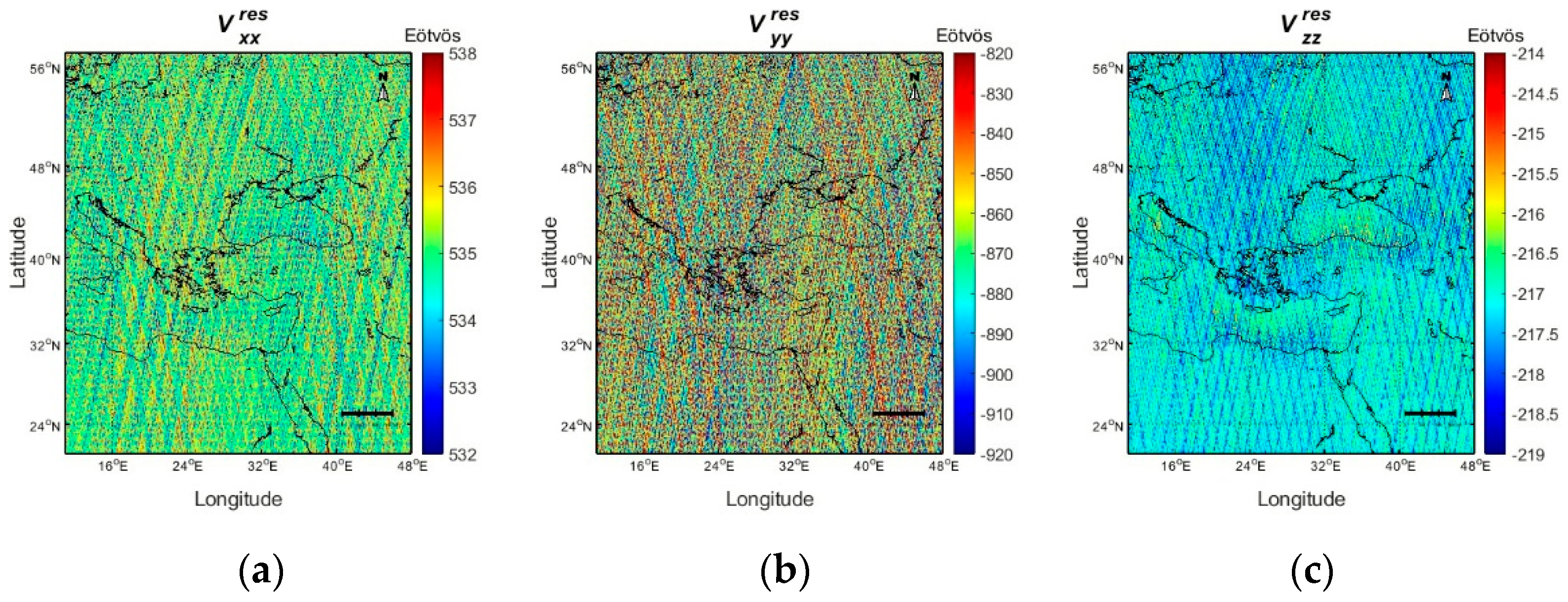
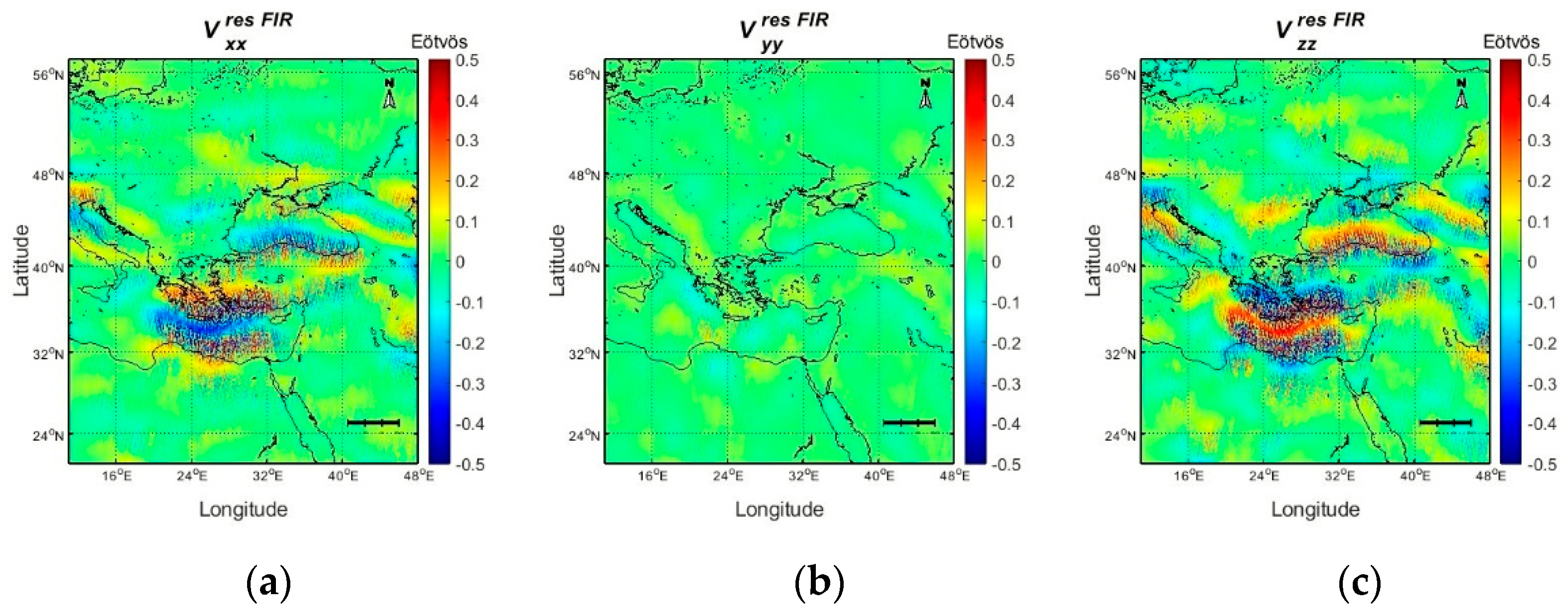
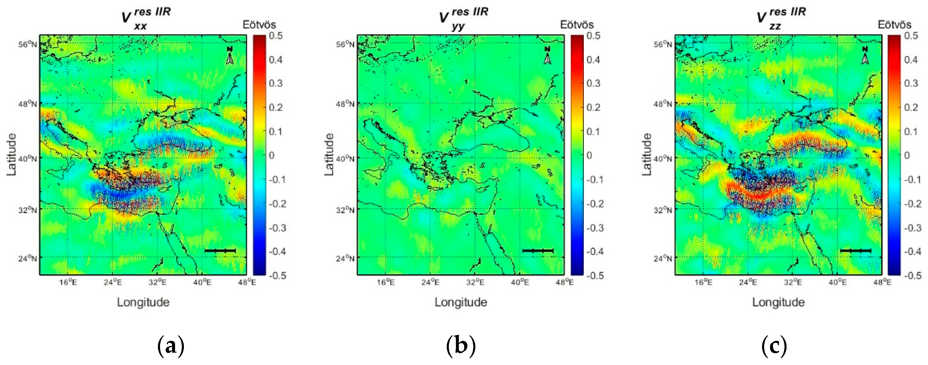
We focus the study on an extended region around Greece, defined as 21° ≤ φ ≤ 57° and 11° ≤ λ ≤ 48°. Figure 1 displays the computed residuals , and for one year’s worth of GOCE data in the study area, while Table 1 summarizes the statistics before and after the reduction of GOCE observations. After the reduction, the std of the estimated residuals is reduced by 66.8% for the 89.2% for , while it increased by 14% for Despite the fact that the component is expected to have the smallest contribution, in the original GOCE observations it is evident that some blunders still exist. Hence, the increase of std after the reduction does not raise questions about the quality of the GGM, but it rather dictates that the data are quite noisy (compare also the residual fields in Figure 1). It should be noted that the entire analysis with the FIR, IIR and WL filters is performed globally, i.e., for the entire one-year record of GOCE data at a global scale. This is preferable for the FIR and IIR filter to avoid edge effects and mandatory for the WL filters as it is applied in the along-track direction of the satellite orbit (see Section 5).
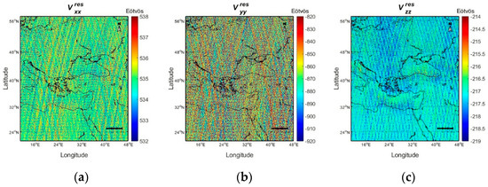
Figure 1.
The gravity gradient residuals (Eötvös) in the Gradiometer Reference Frame for (a) , (b) and (c) .

Table 1.
Statistics of the gravity gradient (GOCE, GGM, and residuals) in the Gradiometer Reference Frame. Units: [Eötvös].
3. Finite Impulse Response (FIR) Filter Design
In order to filter the time series of GOCE gravity gradient residuals, a band-pass, windowed, feed-forward FIR filter was developed according to GOCE measurement bandwidth specifications. The first step to design the filter structure is to determine the frequency response and calculate the filter coefficients. The frequency response of the filter is a rational function of , which can be written as the convolution sum [18,19]:
where the coefficients and define the filter frequency response and is a complex exponential. Note that the terms of the denominator polynomial are zero in the difference equation; therefore, there are no poles (denominator’s roots). Hence the designed filter is non-recursive and there is no feedback, so it is always stable [20,21].
The direct form of an Nth order FIR filter can be described through a linear constant coefficient difference equation, which indicates that any output sample depends on the N input samples, exclusively [22] as:
where denotes the input signal, denotes the output signal, N represents the order of the filter, coefficients indicate the value of the impulse response, and k is the instant for of the order filter. It is noticed that the filter coefficients are computed through a least-squares approximation.
As the filter is structured, a ripple effect, known as Gibbs oscillations, is shown in the transition bands in both passbands. In order to attenuate these oscillations and provide more accuracy to the original frequency spectrum, a window function, such as a Hanning, Hamming or Blackman window [23], with no abrupt discontinuity, should be applied. We chose to apply a Hamming window to eliminate this error and smooth the filter’s impulse response at the edges of the GOCE MBW. The shape of the window and its cutting off frequency is given by [19]:
The final filter coefficients are then derived by multiplying the coefficients with the window function . The effect of applying the window in Equation (4) to the filter frequency response is given by the convolution:
where denotes the desired frequency response, denotes the initial frequency response, represents the Fourier transform of the Hamming window , and symbolizes the convolution.
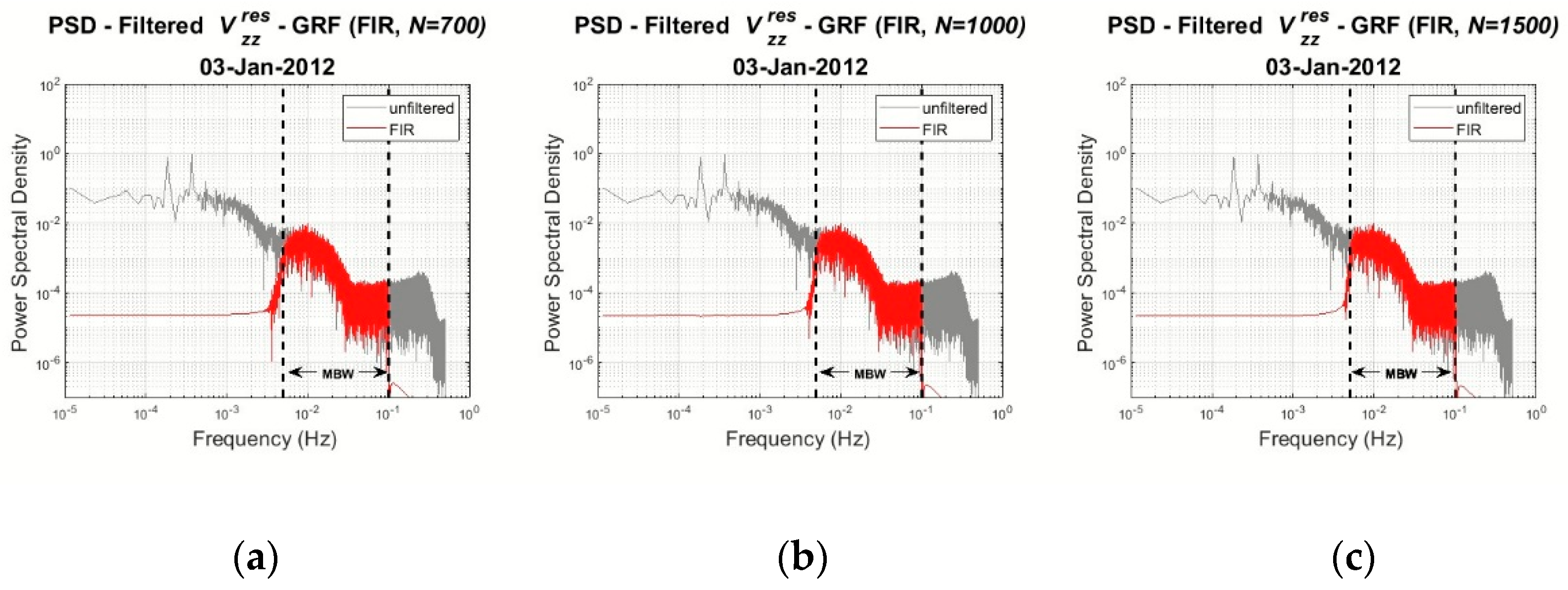
Once the final frequency response has been determined, the filter is applied to the daily GOCE data, separately for each gravity gradient residual . The frequency response of the resulting Nth filter is evaluated in terms of the PSDs of the unfiltered and filtered signals. Figure 2 presents the PSDs of the filtered component for and filter order, respectively. The vertical dashed lines in the figures below designate the cut-off frequencies (0.005 Hz to 0.1 Hz) of the band-pass filter.
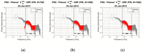
Figure 2.
PSDs of the filtered (red) and unfiltered (grey) residuals for (a) N = 700, (b) N = 1000 and, (c) N = 1500 filter order.
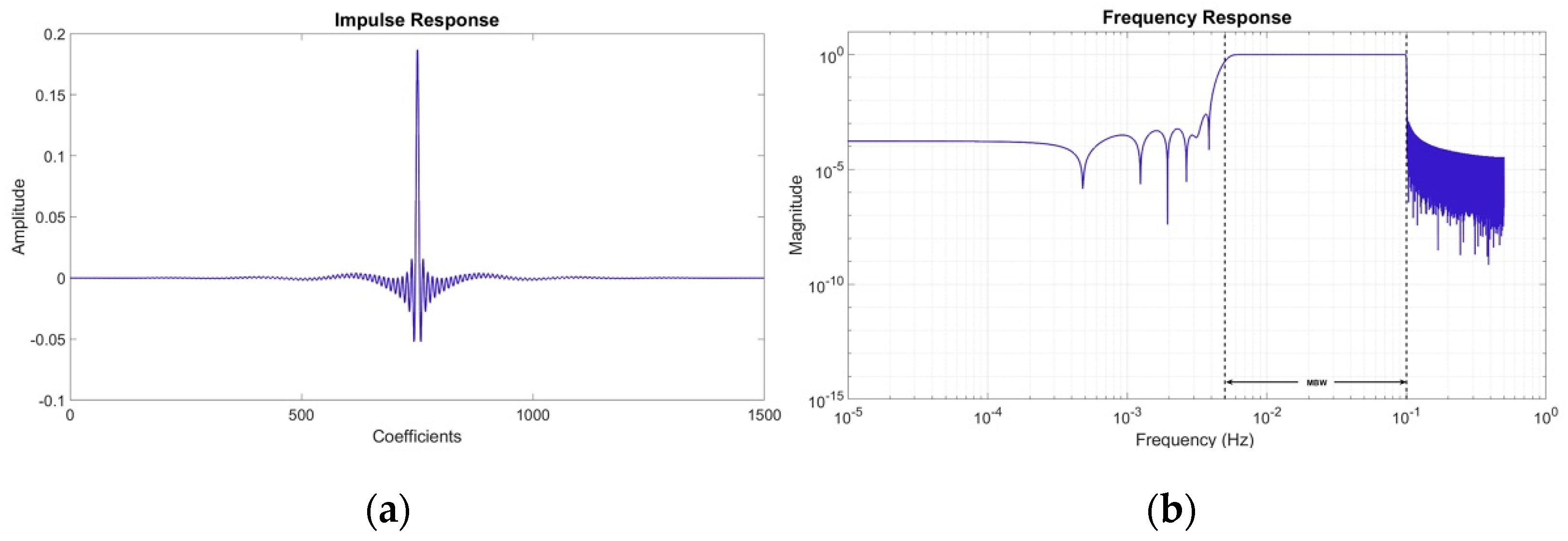
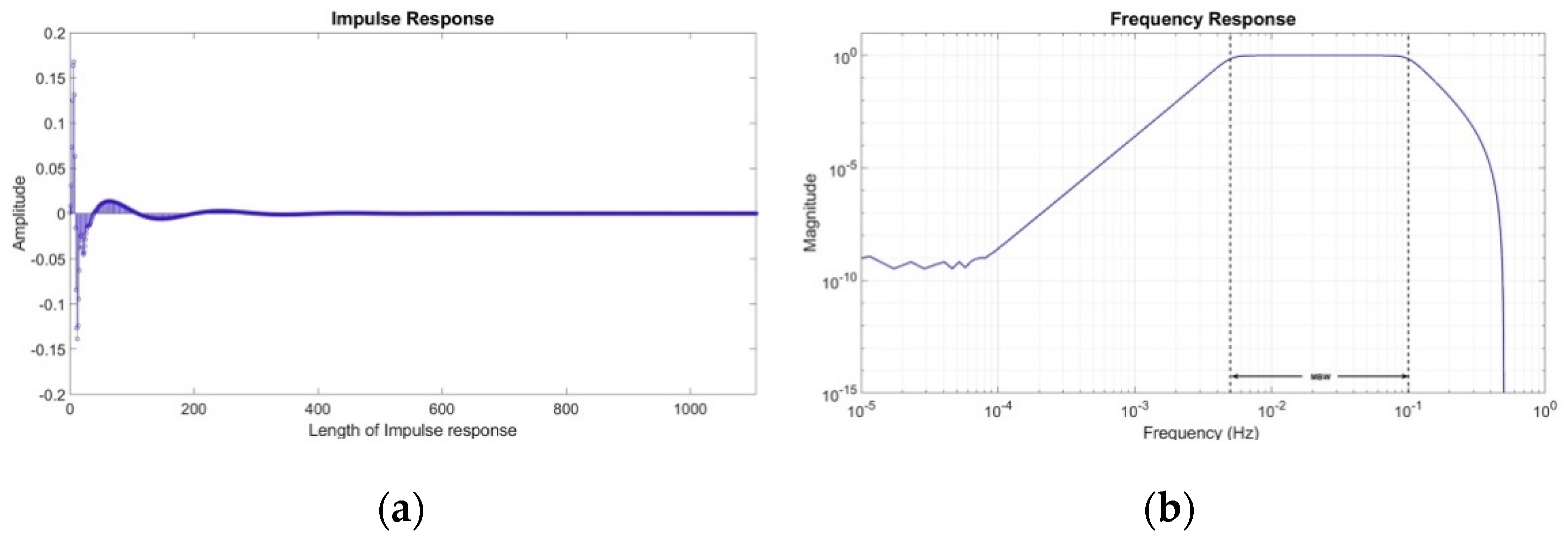
From Figure 2 it can be concluded that the signal remains stable within the GOCE MBW for all filter options, while for lower orders the unfiltered signal remains outside the MBW. Based on this, an FIR filter with order has been selected with its impulse and frequency response being depicted in Figure 3 and Figure 4 outlining the entire windowed FIR filter design procedure.
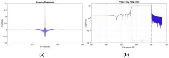
Figure 3.
(a) Impulse Response and (b) Frequency Response of a 1500th order FIR filter.

Figure 4.
FIR filter design procedure.
FIR Computational Experiments
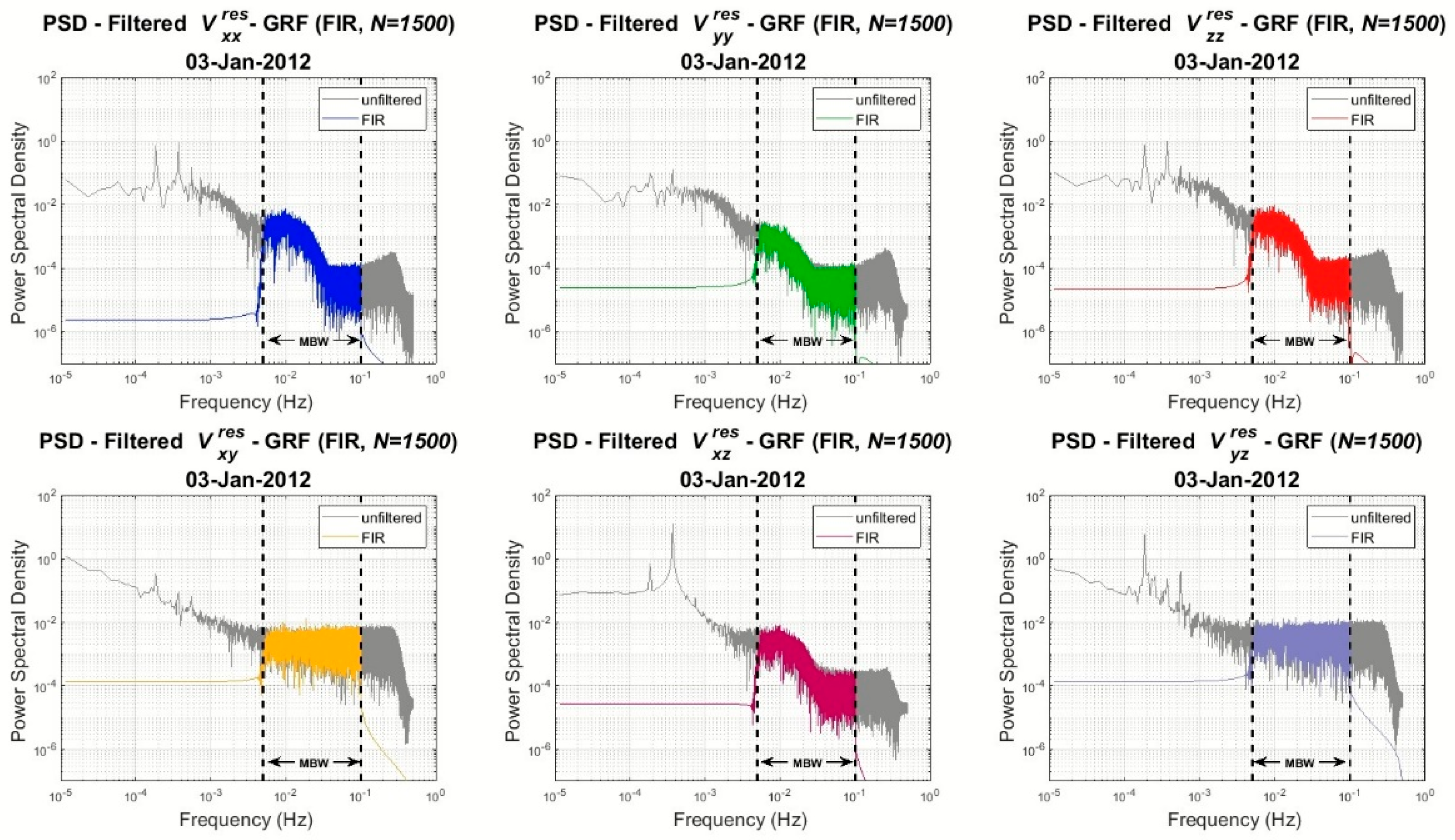
The gravity gradient residuals are filtered with a 1500th order FIR filter. Figure 5 displays the PSDs of the filtered and unfiltered gravity gradient residuals. It is apparent that GOCE signals remain unaffected in the passband while the low- and high-frequencies outside the MBW are removed efficiently. Note that the filter reacts the same way on all gravity gradient components.
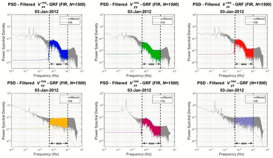
Figure 5.
PSDs of the filtered (colored ones) and unfiltered (grey) gravity gradient residuals for , , , , , .
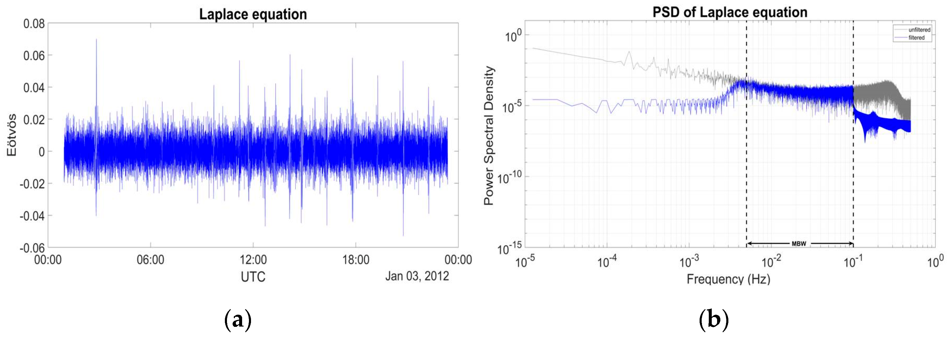
In theory, the trace of the main diagonal gradient components should fulfill Laplace’s equation, i.e., [24]. In order to evaluate the filtering procedure, we compute and analyze the Laplace equation for the filtered gravity gradient residuals. Figure 6 presents their trace in the time and frequency domain, before (gray) and after filtering (blue), while Table 2 summarizes the statistics. In Table 2, FIR denotes the statistics after the application of the FIR filter, IIR the ones after the IIR filter (see Section 4), those after the WL filtering using only levels four to seven for the reconstruction and for those after WL filtering based on selective filtering for and reconstruction with only levels three to seven (see Section 5).
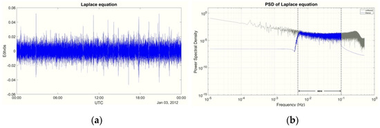
Figure 6.
Trace of the residual FIR filtered SGG tensor in (a) time domain and (b) frequency domain.

Table 2.
Laplace equation statistics for the unfiltered and filtered residuals. Units: [Eötvös].
Ideally, the computed trace of the main diagonal filtered residuals should be zero, as the colored noise has been efficiently removed [25]. As it can be seen from both Figure 6 and Table 2, after the FIR filtering, the mean value of the trace is zero, therefore confirming Laplace’s equation, with a std which is at the ~8 μE level. The latter is a 93.8% reduction of the std of the Laplacian, which together with the zero mean confirm the appropriateness of the FIR filtering. The spectral performance of the filtered residuals, as demonstrated in Figure 6b, implies and confirms that the remaining noise is solely white, as is also shown from the zero mean of the statistics in Table 2. Consequently, it can be concluded that the main diagonal gravity gradient residuals have been filtered correctly and present high quality within the GOCE MBW.
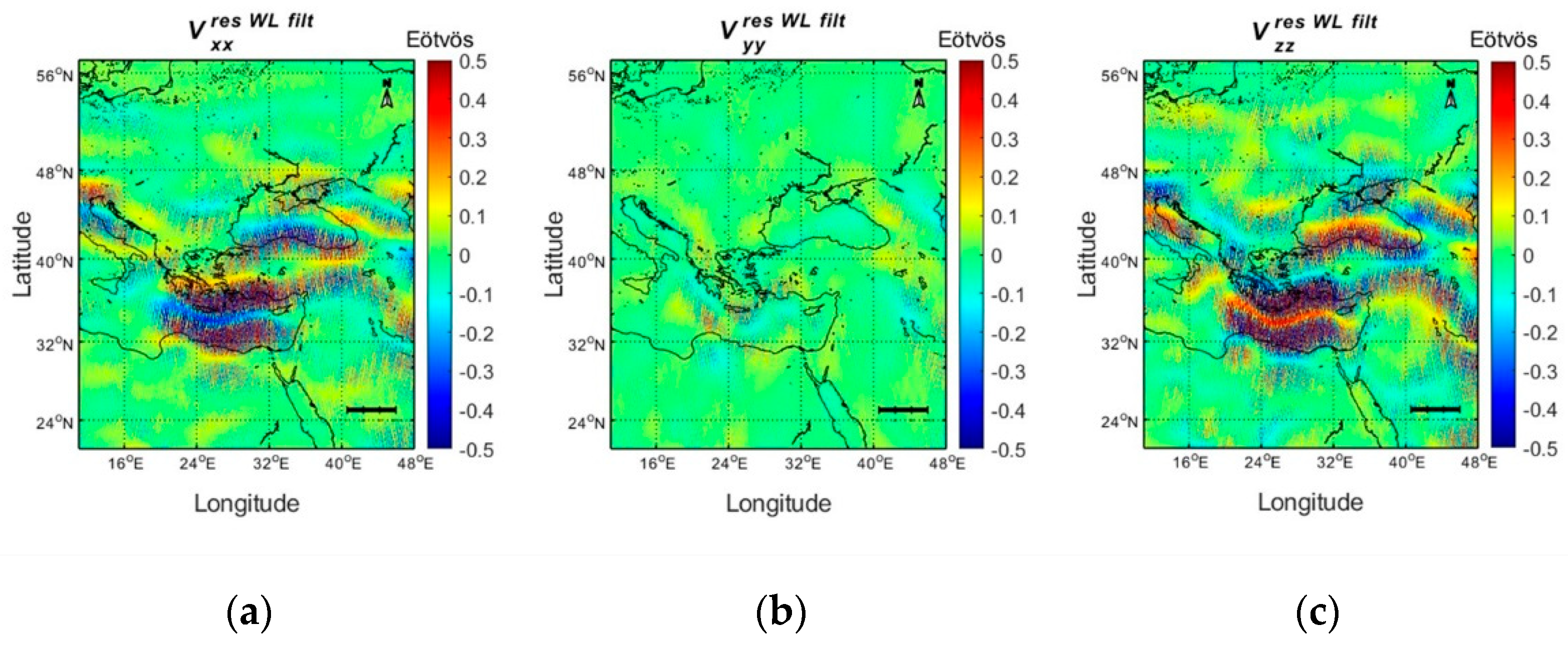
As the result is satisfying, we followed the same process using a 1500th band pass FIR filter for the gravity gradient residuals over a year. We focused the study on an extended region around Greece. Figure 7 presents the filtered in the area under study, while Table 3 summarizes their corresponding statistics. Comparing Figure 1 and Figure 7, where the unfiltered and filtered gradients are presented, it can be concluded that the FIR filtering procedure successfully manages to reduce the track wise errors and the noise in the data. This can be derived from the statistics of the gradients as well (see Table 3), since the std reduces by 91.5% for the 99.8% for and 81.6% for , while the mean value for all gradient gradients is practically zero. This provides good evidence that the FIR filtering is successful, so that the main characteristics of the gravity field in the area under study are well represented, with the dominant feature being the large gradient over the south Aegean Sea.
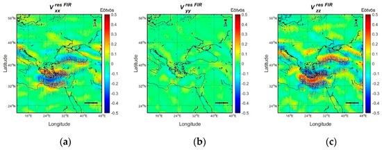
Figure 7.
FIR filtered residuals for components (a) , (b) and (c) .

Table 3.
Statistics of the FIR filtered residuals. Units: [Eötvös].
4. Infinite Impulse Response (IIR) Filter Design
Another type of filter tested to the GOCE time series was through the Infinite Impulse Response (IIR) approach. For this purpose, a digital passband IIR filter based on an analog low-pass Butterworth filter was designed [26]. Five well-known low-pass filters are usually employed in related works, i.e., the Elliptic, Cauer, Bessel, Chebyshev, and Butterworth ones [27]. In this work we have used a Butterworth filter approximation due to its smooth monotonic frequency response , and wide use in the field of geodesy. The filter is given by the following equation:
where denotes the sampling frequency, the cutoff frequency and the order of the filter. Note that an analog () low-pass filter is converted to an equivalent digital passband filter through the z-transform [28]. Also, it should be mentioned that due to the main characteristic of the Butterworth filter, its response is flat and there are no ripples in the passband (0.005 Hz to 0.1 Hz); therefore, no extra window function is needed. The frequency response of an IIR filter can be given as the following convolution sum [18,19]:
where denotes the feed-forward coefficients, denotes the feedback coefficients, and stands for the complex exponential. Considering that the frequency response has both zeros (numerator’s roots) and poles (denominator’s roots), the filter is recursive, so there is feedback on the system. As feedback exists on the system, its stability depends on the poles and their position in the unit circle.
The direct form of an IIR filter can be expressed through the following difference equation:
where denotes the input sample, the related output sample and the auto-regressive part of the filter.
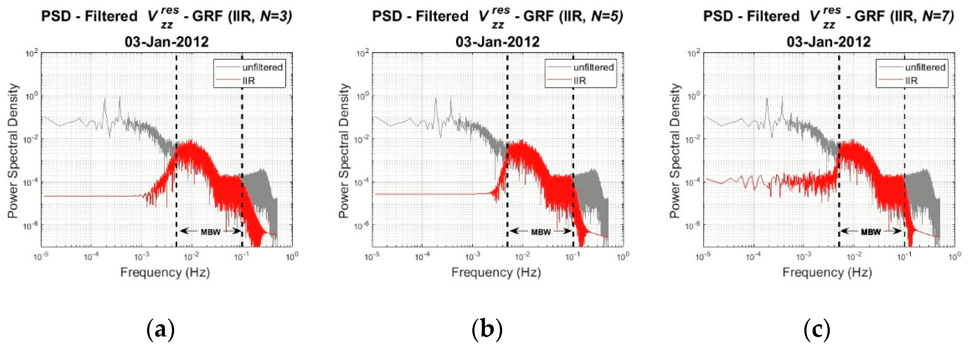
Once the frequency response and the filter coefficients have been determined, the filter is applied to the daily GOCE gravity gradient residuals. As in the case of the FIR filter, the frequency response of the Nth IIR filter is evaluated in terms of the PSDs of the unfiltered and filtered signals. Figure 8 presents the PSDs of the filtered gradients for filter order and .
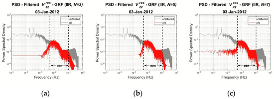
Figure 8.
PSDs of the filtered (red) and unfiltered (grey) for (a) N = 3, (b) N = 5 and, (c) N = 7 filter order.
As shown in Figure 8, the filter can remove the low-frequency errors while preserving the pass-band signals unaffected for each filtering option. However, visible differences are observed. As the filter order increases, the IIR Butterworth filter becomes less efficient in the lower limit of the measurement bandwidth, i.e., frequencies smaller than 0.005 Hz. To investigate the IIR filter stability, the pole configuration has been determined, as shown in Figure 9.

Figure 9.
Pole configuration of for bandpass filter order (a) N = 3, (b) N = 5 and, (c) N = 7.
Given that the poles are enclosed to the unit circle, we can conclude that the system is stable. It is noticed that for each complex pole that there is another conjugate one. Also, it should be mentioned that for filter order N > 7 the poles are located outside of the unit circle and the system becomes automatically unstable. As we confirmed the filters’ stability, we based our study only on their spectral representation. We preferred to use the N = 5 IIR filter, as it has sharper transition characteristics, attenuates high frequencies more efficiently, and reveals the best spectral performance compared to the other options. The IIR filter impulse and frequency response are presented in Figure 10.
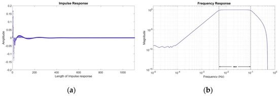
Figure 10.
(a) Impulse response and (b) frequency response of = 5 IIR Butterworth filter.
To conclude, Figure 11 recapitulates the passband Butterworth IIR filter design procedure.

Figure 11.
IIR filter design procedure.
IIR Computational Experiments
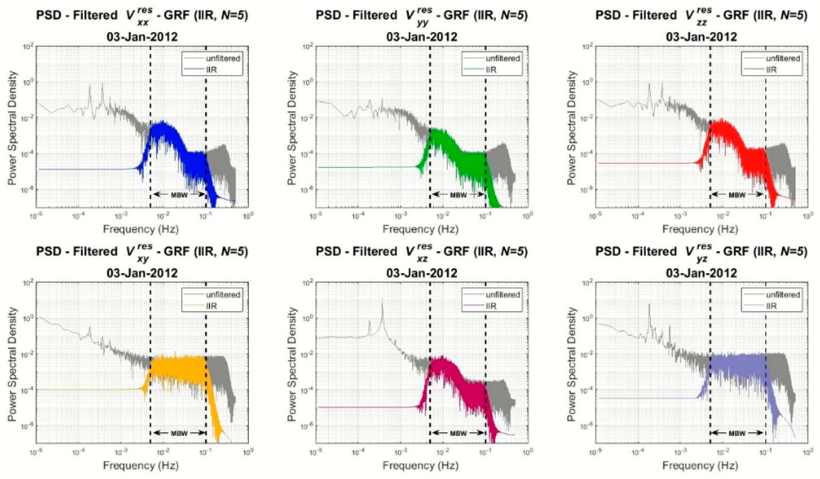
In the practical implementation of the IIR filter, the GOCE gravity gradient residuals are filtered with a 5th order IIR filter. Figure 12 presents the PSDs of the filtered and unfiltered gravity gradient residuals, where it becomes clear that the input signals remain unaffected in the passband, while the low- and high-frequency signal outside the MBW is removed. It should be noticed that the filter responds the same way on all gravity gradient components, while compared to the FIR filter, the IIR does not manage to filter the GOCE signal exactly on the borders of the MBW. In that way, part of the residual signal remains even after filtering. In order to evaluate the IIR filtering, the Laplace equation for the filtered gravity gradient residuals has been computed, with Figure 13 showing their trace in the time and frequency domain and Table 2 giving the respective statistics. Despite the fact that the IIR filter does not manage to filter the GOCE signal exactly on the MBW, the statistics of Laplace’s equation are marginally the same as those with the FIR filter in terms of the range and the std, respectively. As shown in Figure 13 and Table 2, the trace of the main diagonal components has a zero mean value and an std reduced by 94%. The spectral performance of the filtered residuals verifies that the remaining noise is simply white.

Figure 12.
PSDs of the filtered (colored ones) and unfiltered (grey) gravity gradient residuals for , , , , , .

Figure 13.
Trace of the residual IIR filtered SGG tensor in (a) time domain and (b) frequency domain.
The same strategy as in the FIR case was followed when testing the 5th order bandpass Butterworth IIR filter, i.e., the filtering referred to the residual GOCE gradients using one-years’ worth of data. Figure 14 depicts the and Table 4 their statistics over the area under study. Comparing Figure 1 and Figure 14, the main gravity field features over the south Aegean Sea are well-depicted, as well as the strong gradient over the Alps in North Italy. Compared to the FIR filter, the IIR provides almost the same statistics of the filtered residual field. The field is slightly noisier than the FIR one, with a larger range by 9.3 mE, a larger mean by 0.2 mE, and a smaller std by 0.4 mE, but these values are statistically insignificant.
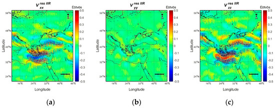
Figure 14.
IIR filtered residuals for components (a) , (b) and (c) .

Table 4.
Statistics of the IIR filtered residuals. Units: [Eötvös].
5. Wavelet MRA Filter Design
The third filtering method used to filter the GOCE gravity gradient residuals was based on wavelets (WLs) in the form of the so-called Wavelet Multi-resolution Analysis (MRA) [29]. Wavelet MRA, both one dimensional (1-D) and two dimensional (2-D), has been extensively used since its introduction in applications of geodesy and gravimetry as a significant analysis tool [30]. WL-MRA has been used in local geoid determination employing gravity anomalies and deflections of the vertical [31] for the evaluation of the Stokes and Vening Meinesz integrals [32], for terrain correction [33], in analysis of GOCE and GRACE based global geopotential models [34], and in GOCE SGG data processing [35]. The localization parameters of the method are its distinctive characteristic, compared to the Fourier transforms which is the standard tool used in signal processing, given the fact that they analyze the signal in both the space and time domains. When employing WLs to analyze potential field data, the selection of the appropriate mother wavelet is important [36]. In the present study, we have employed the Daubechies mother wavelet [37] and in particular the Daubechies 10 (db10) wavelet. The db10 wavelet has been selected due to its smoothness [35], which allows its use with gravity-field related data. Other mother wavelet functions can be employed as well, such as the Haar and the Morlet wavelets, but have not been investigated here as they have proved to provide less accurate results when GOCE SGG data was evaluated against GNSS/Levelling observations. In the frame of the present study, WL-MRA has been used within two schemes. The first one employs wavelets to decompose the GOCE SGG residuals and reconstruct the signal based on the selection of some level of decomposition. The second scenario involves, after the decomposition, selective filtering at the levels referring to the high-frequency information, in order to retrieve signal that is contaminated by noise. Such a selective filtering approach using wavelets alongside with classical filtering can provide further improved results [38].
As in the FIR and IIR cases, the computed GOCE residual data were filtered using wavelets with the purpose of retaining the signal inside the MBW of the satellite. The GOCE data needed to first be divided into orbits in order for the wavelet functions to be applied in the along-track direction. For each orbit, the satellite required 1.5 h, or 5400 s, meaning that sixteen orbits were fulfilled in a single day. This results in a typical daily file of GOCE that includes sixteen orbits (86,400 s), fifteen full and two half orbits, one at the start and one in the end of the file. Wavelet decomposition decomposes the original signal in levels and each of these levels corresponds to a specific spatial resolution. The spatial resolution of every level is the double of the previous one, and the number of levels is selected so that the spatial resolution of the last level corresponds to the perimeter of the Earth in spherical approximation. For each level of decomposition in the 1-D wavelet analysis, detail and approximation coefficients are computed. The detail and approximation coefficients are computed by the wavelet (ψ) and the scaling functions (φ), respectively. The GOCE gravity gradiometer collects measurements at an interval of 1 s which, based on its speed, corresponds to an 8 km measurement rate [35] and to a spatial resolution varying from 8 to 16 km for the first level. Table 5 summarizes the correspondence between decomposition levels and spatial resolution. Given that the latest GOCE global geopotential models have a useful bandwidth to degree and order (d/o) 280–300 [39], this corresponds to a spatial resolution of ~70 km, implying that the useful levels in the WL-MRA would be from level 4 and above.

Table 5.
Resolution of the levels of decomposition.
The selection of levels to be removed or retained is dictated each time by the objectives of the filtering procedure. Such would be the case of removing high-frequency signal (first levels of decomposition) or retaining the low-frequency one (higher levels of decomposition).
In general, the signal reconstruction is based on a summation that includes the detail coefficients, which need to be retained, and the approximation coefficient of the last level of decomposition. A key role that allows this simple signal reconstruction is the orthogonality property of wavelets [29,30]. Unwanted levels are accordingly omitted from the reconstruction process and their impact on the newly synthesized signal is excluded. The following equation represents a signal reconstruction, where () are the detail coefficients of each level of decomposition, the approximation coefficient of the last level (in this case the twelfth one), and is the reconstructed signal.
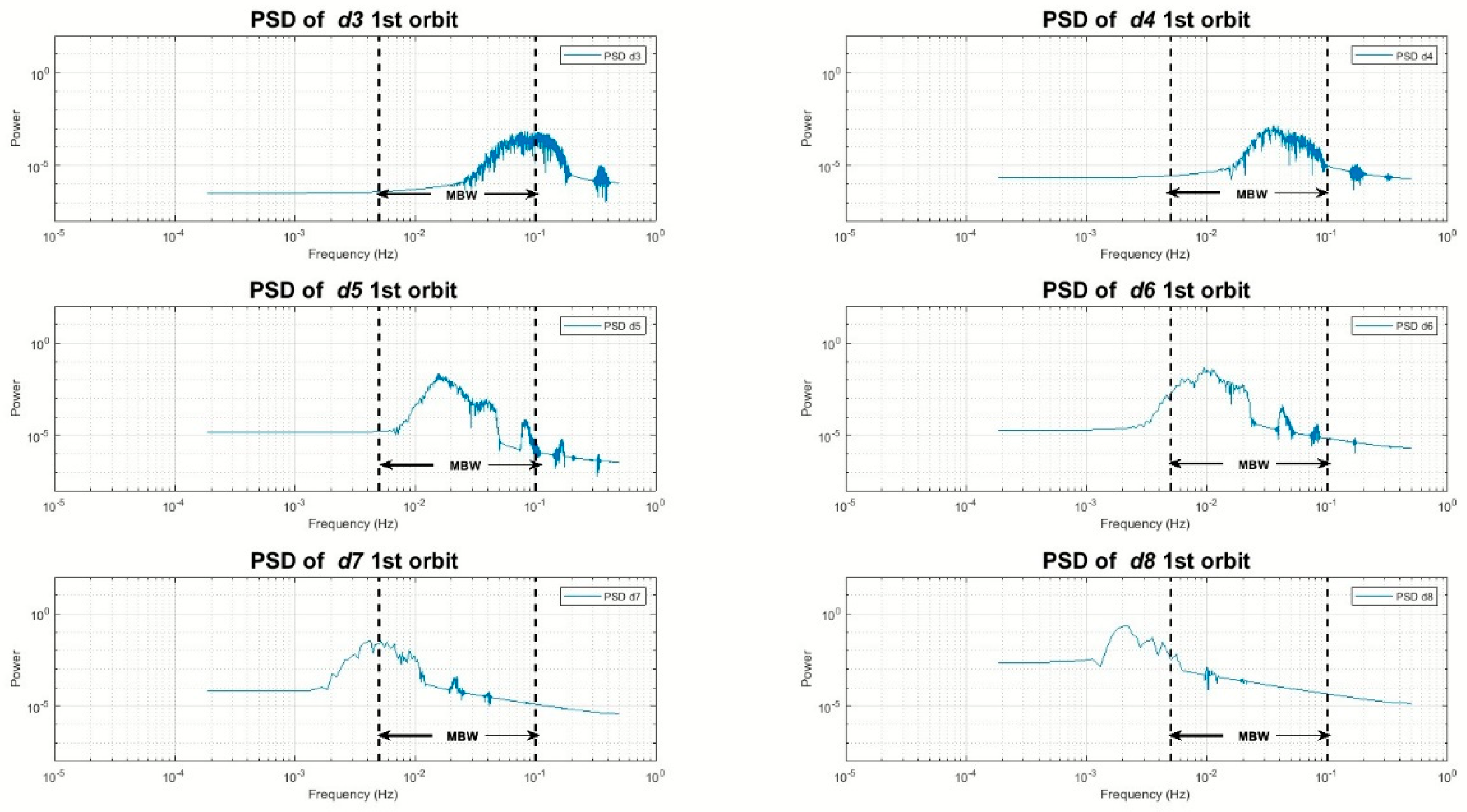
As already mentioned, the mother wavelet used in the present study was a Daubechies one (db10) with twelve levels of decomposition. PSDs for all the coefficients of decomposition were calculated and plotted for an orbit of the satellite so as to distinguish the relation between the spectral content of each level and the satellite MBW. It was found that detail coefficients from levels (l) l4 to l7, corresponding to spatial resolutions from 64 to 1024 km were the ones that mainly carried the signal inside the MBW in all six of the gravity gradients. Figure 15 depicts the signal PSDs for l3 to l7 detail coefficients, which mainly include information inside the GOCE MBW. From Figure 15 it can be clearly seen that detail coefficients from levels larger than 7 do not contain information within the MBW (see l8 PSDs), hence they should not be included in the reconstruction. On the other hand, the l3 coefficients have signal marginally within the upper band of the MBW spectrum. For the l3 contribution, we are most interested in the signal from 4∙10−2 Hz to 10−1 Hz, which seems to be within the MBW complementing the l4 signal which loses its power in that band (see the decay of the l4 signal after 3 × 10⁻² Hz).
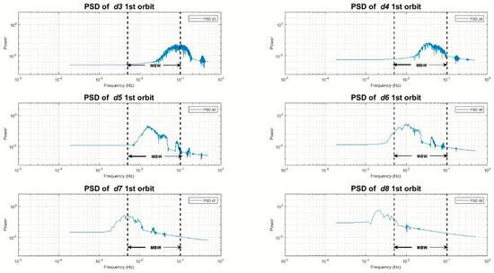
Figure 15.
PSDs of detail coefficients of levels 3, 4, 5, 6, 7 and 8 (d3, d4, d5, d6, d7, and d8) for one orbit of the Vzz component.
Based on the above, various scenarios concerning signal reconstructions using different combinations of detail coefficients were applied to daily files, with a reconstruction using only the detail coefficients of levels 4 to 7 being the one that optimally retained the useful signal, as it excluded higher and lower frequencies outside the MBW. Retaining the signal outside the MBW introduces errors that affect the final filtered data. These errors would then be propagated to the next processing steps, such as gravity anomaly and geoid estimation.
Figure 16 presents the PSDs of three reconstruction scenarios based on l3 to l7, l4 to l7 and l4 to l8, respectively. As it can be seen, the use of l3 retains a signal outside the MBW towards the higher frequencies (10−1 to 2 × 10⁻¹ Hz), while the use of l8 retains signal in the lower frequencies (5 × 10⁻³ to 2 × 10⁻³ Hz). Figure 17 outlines the WL-MRA processing scheme as employed for GOCE SGG filtering.
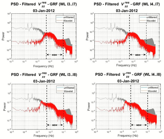
Figure 16.
PSDs of the filtered (red) and unfiltered (grey) gravity gradient for reconstruction l3..l7 (top left), reconstruction l4..l7 (top right), reconstruction l4..l8 (bottom left), and reconstruction l4..l8 (bottom right).

Figure 17.
Wavelet MRA design procedure.
Wavelet MRA Computational Experiments
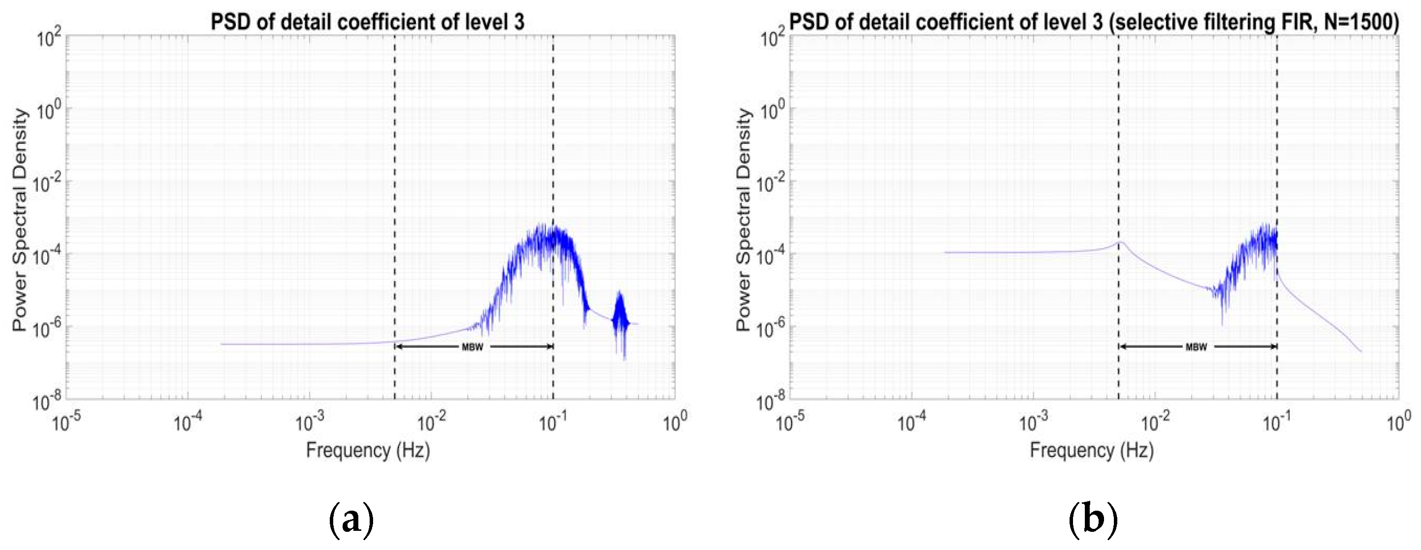
Based on the previous characteristics of the signal PSDs for the detail coefficients, the following scenarios have been tested for GOCE SGG filtering. First, signal reconstruction was based on the use of l4 to l7 given that this combination retains a signal only within the MBW (see Figure 16). A second scenario was based on selective filtering of l3, in order to retain some higher frequencies between 6 × 10⁻² and 10−1 Hz. The selective filtering of l3 detail coefficients is based on the aforementioned FIR filter with . Figure 18 shows the PSD of the l3 detail coefficients before and after selective filtering, while Table 6 and Table 7 show the respective statistics. From Figure 18 it can be seen that after the selective filtering signal inside the MBW is mainly retained in the detail coefficients of level 3, while the noise of the higher frequencies is removed. From Table 6 and Table 7 it can be seen that the selective filtering applied to l3 reduces the std by 27% for , 26% for and 25% for .
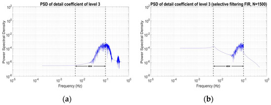
Figure 18.
PSDs of detail coefficients of level 3 (a) before and (b) after the selective filtering for one orbit of the component.

Table 6.
Statistics of the detail coefficient of level 3 before the selective filtering. Unit: [Eötvös].

Table 7.
Statistics of the detail coefficient of level 3 after the selective filtering. Unit: [Eötvös].
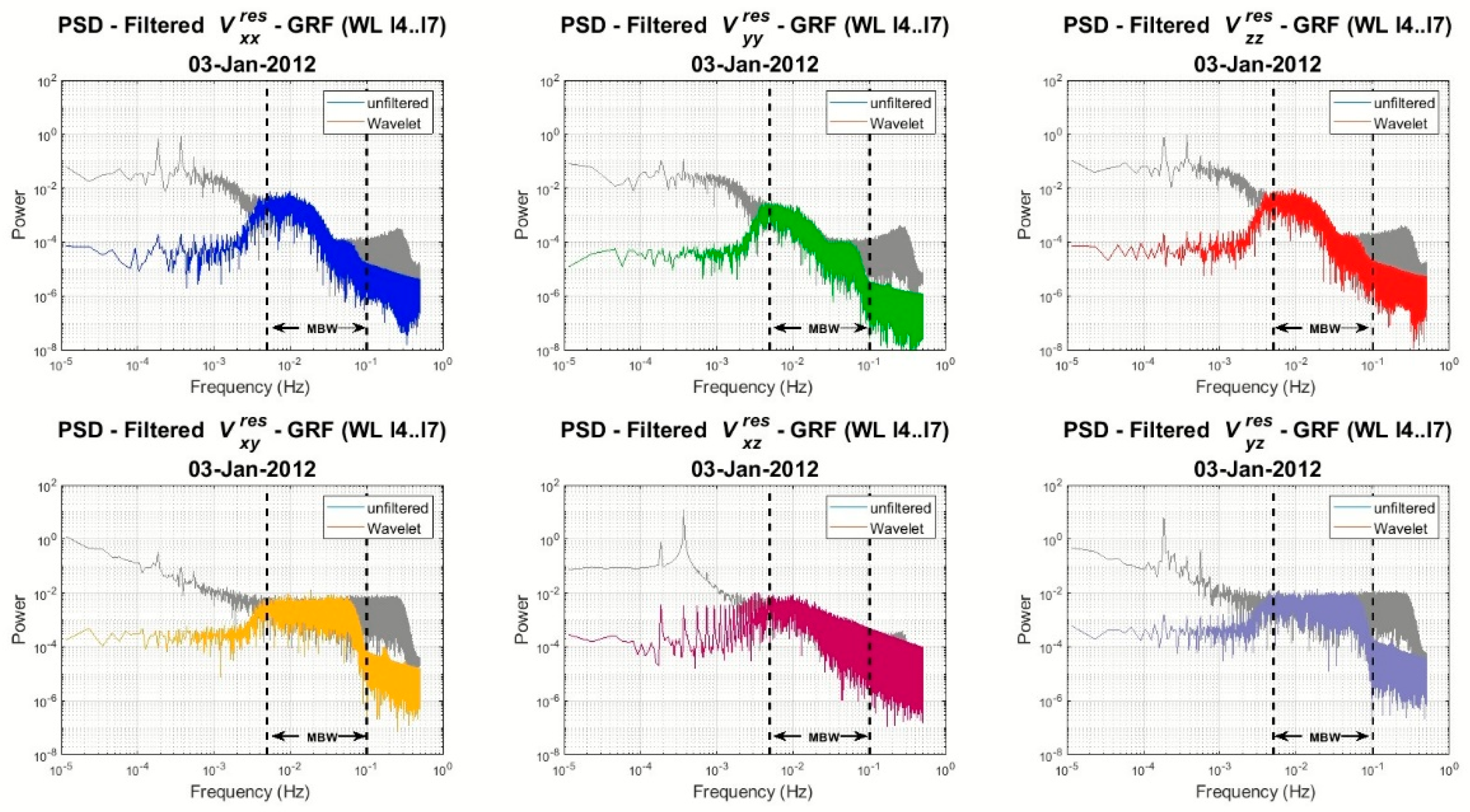
Based on the aforementioned results, a more representative behavior of the two optimal WL filters, meaning reconstruction l4..l7 and reconstruction of l3filtl4..l7, is illustrated in Figure 19 and Figure 20, where the PSDs for all the gravity gradient residuals are depicted. As can be seen, the reconstruction of l4..l7 presents some distinct steps in the higher bands of the spectrum (see the bandwidth from 4 × 10⁻² to 10−1 Hz. This indicates that l4 alone cannot provide the higher frequencies to the end of the spectrum. From Table 5 the spatial extent of l3 reaches 64 km, which corresponds to the harmonic degree (d/o) of expansion ~310. Even the latest GOCE GGMs, such as TIM-R6, reach a maximum d/o of 300, since after that the signal to noise ratio of the spherical harmonic coefficients is lower than 1 [40]. This is an interesting point, since formally l3 should not fall within the MBW of GOCE. Nevertheless, after selective filtering of l3 and reconstruction (see Figure 20) the filtered signal PSD seems more compete without any steps inside the MBW.
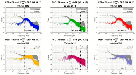
Figure 19.
PSDs of the filtered (colored ones) and unfiltered (grey) gravity gradient residuals after reconstruction l4..l7 for , , , , , .
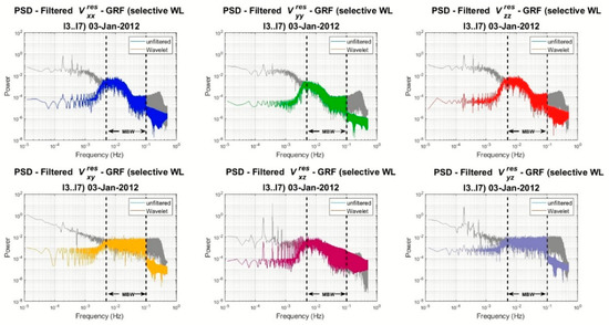
Figure 20.
PSDs of the filtered (colored ones) and unfiltered (grey) gravity gradient residuals after selective reconstruction l3filtl4..l7 for , , , , , .
Another useful measure to evaluate the filtering procedure it to compute Laplace’s equation using the filtered diagonal gravity gradients for the two reconstruction scenarios. The results of the Laplace equation, as well as its PSD and statistical behavior, are shown in Figure 21 and Figure 22 and Table 2 for both tests. The l4..l7 reconstruction provides results with lower std from the FIR and IIR filters, but as seen from Figure 21 the signal strength is lost at the higher frequencies of the MBW. This is corrected when using selective filtering for l3 and then performing the reconstruction with l3filtl4..l7.
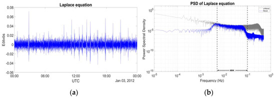
Figure 21.
Trace of the residual WL MRA filtered SGG tensor of the reconstruction l4..l7 for one day of data in (a) time domain and (b) frequency domain.

Figure 22.
Trace of the residual WL MRA filtered SGG tensor of the selective reconstruction l3filtl4..l7 for data of 15 full orbits in (a) time domain and (b) frequency domain.
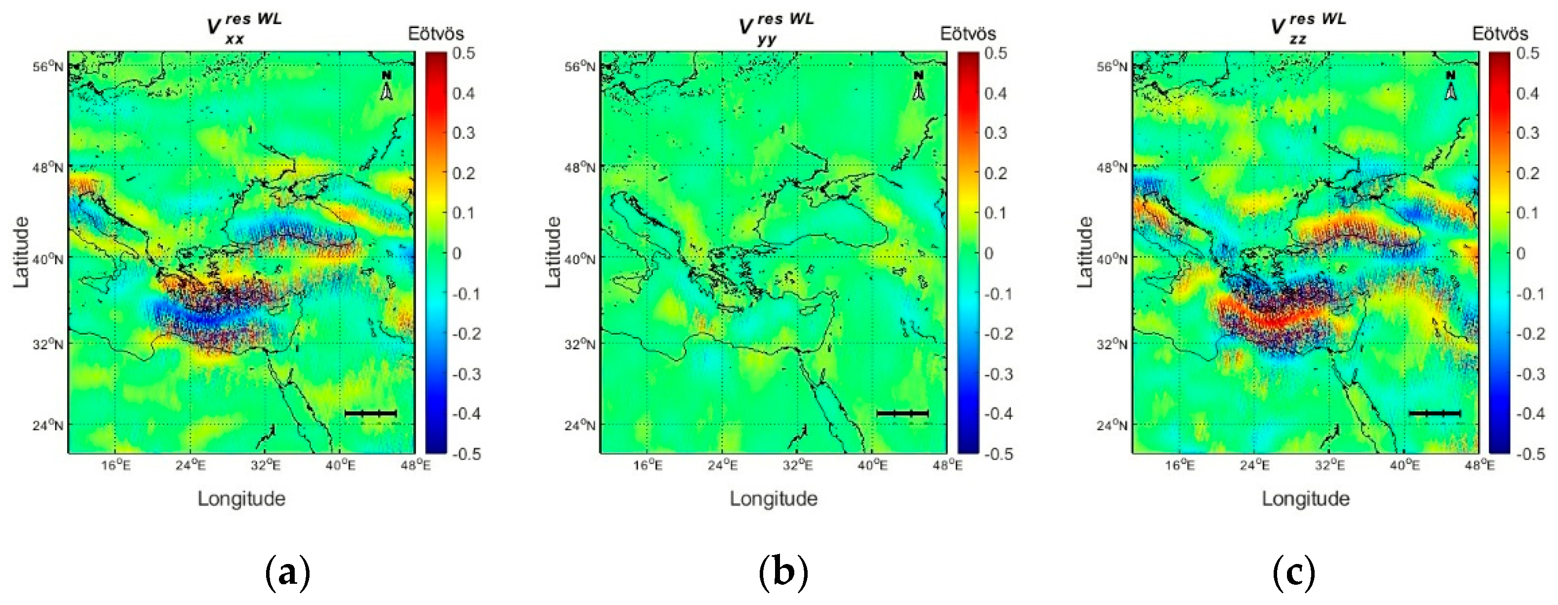
Finally, one-years’ worth of GOCE data were filtered based on the WL MRA with the resulting field depicted in Figure 23, for the three diagonal residual gravity gradients. The statistics are presented in Table 8, where it can be seen that the mean is at the 0.1–0.4 mE level for all constituents. WL MRA gives almost the same filtered residuals with the more traditional FIR and IRR filters, with slightly lower std by 5 mE for , 0.3 mE for , and higher std by 4 mE for . The range of the MRA residuals are higher compared to the classical filters by as much as 1.8 E for the , which is depicted in Figure 23 (see panel c) along with a stronger signal, especially over the Eastern Mediterranean Sea.
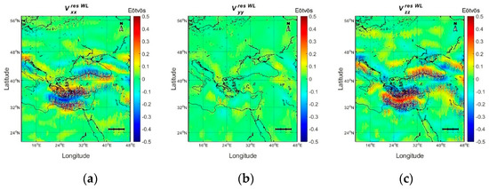
Figure 23.
The l4..l7 reconstruction based on one year of residual data (a) , (b) and (c) .

Table 8.
Statistics for the l4..l7 reconstruction for one year of data. Unit: [Eötvös].
The same scenario was carried out with selective filtering using the reconstruction l3filtl4..l7 and FIR 1500 for one year of GOCE data as shown in Figure 24 and Table 9. The reconstructed signal appears to have the same characteristics as the simple l4..l7 reconstruction, and close to the classic FIR and IIR filters. The main difference of the l3filtl4..l7 residual signal, compared to the l4..l7 synthesis, is in the range of all constituents, which is higher by 1–4 mE.

Figure 24.
The selective l3filtl4..l7 reconstruction based on one year of residual data (a) , (b) and (c) .

Table 9.
Statistics for the selective l3filtl4..l7 reconstruction for one year of data. Unit: [Eötvös].
To evaluate the differences between the filtered fields, Figure 25 depicts the comparison between the FIR, IIR, WL MRA and filtered WL MRA residuals, while Table 10 tabulates the statistics. As it can be seen, the FIR and IIR filters give almost the same results with a std of the differences at the 11 mE level. The differences with the l4..l7 synthesis are much higher with an std 4–5 mE and a range of 300–400 mE. This is also depicted in Figure 25, where the differences show a strong orange-skin effect with variations in the form of tesseral harmonics from −0.1 E to 0.1 E. The spatial extent of these features is ~7° × 7°, which corresponds to ~770 km and coincides with the l8 coefficients which are omitted from the WL synthesis. Despite the fact that they are very small in magnitude, it shows that there is still some residual signal not filtered by the FIR and IIR in the edges of the GOCE MBW. Moreover, the shorter scale characteristics show that the l4..l7 synthesis, without inclusion of the l3 contribution (see also the steps in the Figure 16 PSDs), does not manage to map the shorter scale characteristics in the higher frequencies of the GOCE MBW. This is smoothed out in the comparisons of the l3filtl4..l7 residuals with those from the FIR and particularly the IIR. In this latter comparison, the strong signal differences are smoothed out, compared to the simple l4..l7 synthesis, which is evidenced in the statistics as well, with a reduction of the range to the FIR by 3 mE and to the IIR by 1 mE. The differences between the FIR and IIR residuals have a range of ~80 mE and a std of 11 mE and show differences mainly in the form of tesseral harmonics. Finally, the differences between the residuals of the two WL filters have a range of 32 mE and an std of just 3 mE. The aforementioned differences between the FIR, IIR and WL filtered residuals, which are at the sub mE level in terms of the mean and at the 10–40 mE level in terms of the std signal that the three alternatives tested, provide compatible results.
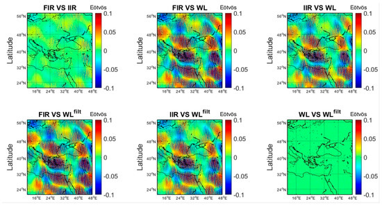
Figure 25.
differences between the FIR, IIR, WL and WLfilt residuals for FIR vs. IIR, FIR vs. WL, IIR vs. WL, FIR vs. WLfilt, IIR vs. WLfilt, and WL vs. WLfilt.

Table 10.
Statistics of differences between the FIR, IIR and WL MRA filtered residuals. Unit: [Eötvös].
6. Conclusions and Discussion
Three different strategies to filter GOCE SGG data to the mission MBW have been discussed in this study, ranging from the classic FIR and IIR filters to a novel WL filter employing the db10 wavelet. The filters have been applied to the actual GOCE gravity gradient residuals, after reduction to a spectrally enhanced version of TIM-R6 with EGM2008, aiming to reduce noise outside the MBW. The most suitable parameters of each filtering technique were identified through various numerical experiments. From the results acquired, the optimal choice for the Finite Impulse Response filter was a 1500-order filter, for the Infinite Impulse Response a five-order filter, and for the Wavelet MRA a reconstruction using the detail coefficients of levels four to seven. In the latter case, selective filtering of the l3 detail coefficients gave improved results, as it both managed to produce signal PSDs without any steps in the higher frequencies of the MBW and provided smallest differences with the FIR and IIR filters. It should be noted that the filtering outputs are the direct results, and no further processing was performed in order to smooth-out residual noise. Each of the filtering methods showed promising results based on the statistical properties and the satisfactory spectral performance, as all can remove the long-wavelength correlated errors and noise in the GOCE observations. The results acquired, especially in terms of the filtering of the signal within the GOCE MBW and the reduction of the noisy characteristics of GOCE in the space domain are consistent with those achieved in [3,4,5]. The FIR and IIR filtered residuals show an agreement at the 11 mE level, in terms of the std, which increases to ~40–50 mE in comparison with the WL filter. The selective filtering with WLs poses a promising alternative to the classic FIR and IIR ones, as the signal is decomposed in specific spatial scales, and dedicated filtering can be applied directly to each level of decomposition without changes in the other parts of the signal spectrum. This implies that certain high-frequency features present in the GOCE SGG data in the spatial scales 60–70 km (d/o~272–300) can be retained by selective filtering of the l3 detail coefficients.
Author Contributions
Conceptual design of the experiment and analysis, G.S.V. and I.N.T.; FIR and IIR filter design and analysis E.M. and G.S.V.; Wavelet MRA filter design and analysis E.P. and I.N.T.; filter validation and experiment design E.M., E.P., D.A.N., V.N.G.; writing—original draft preparation, E.M., E.P. and D.A.N.; writing—review and editing, I.N.T., G.S.V., V.N.G. and M.G.S.; visualization, E.P., E.M., D.A.N. and G.S.V.; supervision, G.S.V. and I.N.T.; project administration, I.N.T.; funding acquisition, I.N.T. All authors have read and agreed to the published version of the manuscript.
Funding
This research was funded by the Hellenic Foundation for Research and Innovation (H.F.R.I.) under the “1st Call for H.F.R.I. Research Projects to support Faculty members and Researchers and the procurement of high-cost research equipment grant” (Project Number: 3488).
Data Availability Statement
In the frame of the GeoGravGOCE project a dedicated software has been designed, where filtering can be tested as well. The software source code as well as sample 1-day GOCE data can be downloaded from https://github.com/gsvergos/GeoGravGOCE and http://olimpia.topo.auth.gr/GeoGravGOCE/software/software.html (accessed on 10 May 2022) to investigate the filtering tools described in this paper.
Acknowledgments
We gratefully acknowledge the three anonymous reviewers for their constructive comments.
Conflicts of Interest
The authors declare that they have no conflict of interest.
References
- Albertella, A.; Migliaccio, F.; Sansó, F. GOCE: The Earth Gravity Field by Space Gradiometry. Celest. Mech. Dyn. Astron. 2002, 83, 1–15. [Google Scholar] [CrossRef]
- Schuh, W.D. The Processing of Band-Limited Measurements; Filtering Techniques in the Least Squares Context and in the Presence of Data Gaps. Space Sci. Rev. 2003, 108, 67–78. [Google Scholar] [CrossRef]
- Raizner, C. GOCE Data and Gravity Field Model Filter Comparison; ESA: Stuttgart, Germany, 2007. [Google Scholar]
- Reguzzoni, M.; Tselfes, N. Optimal Multi-Step Collocation: Application to the Space-Wise Approach for GOCE Data Analysis. J. Geod. 2009, 83, 13–29. [Google Scholar] [CrossRef]
- Krasbutter, I.; Brockmann, J.M.; Kargoll, B.; Schuh, W.-D. Adjustment of Digital Filters for Decorrelation of GOCE SGG Data. In Observation of the System Earth from Space—CHAMP, GRACE, GOCE and Future Missions; Springer: Berlin/Heidelberg, Germany, 2014; pp. 109–114. [Google Scholar] [CrossRef]
- Kern, M.; Preimesberger, T.; Allesch, M.; Pail, R.; Bouman, J.; Koop, R. Outlier Detection Algorithms and Their Performance in GOCE Gravity Field Processing. J. Geod. 2005, 78, 509–519. [Google Scholar] [CrossRef]
- Gruber, T.; Rummel, R.; Koop, R. How to Use GOCE Level 2 Products; ESA: Paris, France, 2007; pp. 205–211. [Google Scholar]
- ESA. GOCE High Level Processing Facility GOCE Level 2 Product Data Handbook; ESA: Paris, France, 2014. [Google Scholar]
- Salminen, A.; Tompa, F. Fundamentals. In Communicating with XML; Springer: Boston, MA, USA, 2011. [Google Scholar] [CrossRef]
- Arsov, K. GOCEPARSER—A Program to Parse GOCE Level 1b and Level 2 Data. In EGU General Assembly Conference Abstracts; EGU: Munich, Germany, 2012. [Google Scholar]
- Brieden, P.; Müller, J. Validation of GOCE Gravitational Gradients in Satellite Track Cross-Overs. In Earth on the Edge: Science for a Sustainable Planet; Springer: Berlin/Heidelberg, Germany, 2014; pp. 399–405. [Google Scholar]
- Torge, W.; Muller, J. Geodesy; De Gruyter: Berlin, Germany, 2012; ISBN 978-3110207187. [Google Scholar]
- Brockmann, J.M.; Schubert, T.; Mayer-Gürr, T.; Schuh, W.D. The Earth’s Gravity Field as Seen by the GOCE Satellite—An Improved Sixth Release Derived with the Time-Wise Approach (GO_CONS_GCF_2_TIM_R6). GFZ Data Serv. 2019, 3, 1–9. [Google Scholar] [CrossRef]
- Pavlis, N.K.; Holmes, S.A.; Kenyon, S.C.; Factor, J.K. The Development and Evaluation of the Earth Gravitational Model 2008 (EGM2008). J. Geophys. Res. Solid Earth 2012, 117. [Google Scholar] [CrossRef] [Green Version]
- Vergos, G.S.; Erol, B.; Natsiopoulos, D.A.; Grigoriadis, V.N.; Işık, M.S.; Tziavos, I.N. Preliminary Results of GOCE-Based Height System Unification between Greece and Turkey over Marine and Land Areas. Acta Geod. Et Geophys. 2017, 53, 61–79. [Google Scholar] [CrossRef]
- Bucha, B.; Janák, J. A MATLAB-Based Graphical User Interface Program for Computing Functionals of the Geopotential up to Ultra-High Degrees and Orders. Comput. Geosci. 2013, 56, 186–196. [Google Scholar] [CrossRef]
- Mamagiannou, E.M.G.; Pitenis, E.A.; Natsiopoulos, D.A.; Georgios, S. GeoGravGOCE: A GOCE SGG Processing Software for Datum Transformations and Filtering. In EGU General Assembly Conference Abstracts; EGU: Munich, Germany, 2021. [Google Scholar] [CrossRef]
- Oppenheim, A.V.; Schafer, R.W. Discrete-Time Signal Processing, 2nd ed.; Prentice Hall: Upper Saddle River, NJ, USA, 1999. [Google Scholar]
- Hayes, M.H. Schaum’s Outline of Theory and Problems of Digital Signal Processing; Schaum’s Outline Series; McGraw Hill: New York, NY, USA, 1999. [Google Scholar]
- Lai, E. Time-Domain Representation of Discrete-Time Signals and Systems. In Practical Digital Signal Processing; Elsevier: Amsterdam, The Netherlands, 2003; pp. 50–60. [Google Scholar] [CrossRef]
- Grout, I. Digital Systems Design with FPGAs and CPLDs; Elsevier: Amsterdam, The Netherlands, 2008; ISBN 9780750683975. [Google Scholar]
- Tarr, E. Finite Impulse Response Filters. In Hack Audio; Routledge: London, UK, 2018; pp. 205–234. [Google Scholar] [CrossRef]
- Podder, P.; Zaman Khan, T.; Haque Khan, M.; Muktadir Rahman, M. Comparative Performance Analysis of Hamming, Hanning and Blackman Window. Int. J. Comput. Appl. 2014, 96, 975–8887. [Google Scholar] [CrossRef]
- Hofmann-Wellenhof, B.; Moritz, H. Physical Geodesy; Springer Science & Business Media: Berlin, Germany, 2005; ISBN 3211235841. [Google Scholar]
- Yi, W.; Murböck, M.; Rummel, R.; Gruber, T. Performance Analysis of GOCE Gradiometer Measurements. In Proceedings of the ESA Living Planet Symposium, Bergen, Norway, 28 June–2 July 2010; Volume 686, p. 393. [Google Scholar]
- Lyons, R.G. Understanding Digital Signal Processing; Bernard Goodwin: Saddle River, NJ, USA, 2004; pp. 151–183, 212–279. ISBN 0-13-108989-7. [Google Scholar]
- Wanhammar, L. Digital Filters. DSP Integrated Circuits; Elsevier: Amsterdam, The Netherlands, 1999. [Google Scholar] [CrossRef]
- Wanhammar, L. Digital Filters Using MATLAB; Springer International Publishing: Cham, Switzerland, 2020; ISBN 9783030240622. [Google Scholar]
- Mallat, S.G. A Theory for Multiresolution Signal Decomposition: The Wavelet Representation. IEEE Trans. Pattern Anal. Mach. Intell. 1989, 11, 674–693. [Google Scholar] [CrossRef] [Green Version]
- Keller, W. Wavelets in Geodesy and Geodynamics; De Gruyter: Berlin, Germany, 2004; ISBN 9783110198188. [Google Scholar]
- El Habiby, M.M.; Sideris, M.G. A Wavelet Thresholding Technique for Local Geoid and Deflection of the Vertical Determination Using a Planar Approximation. Geophys. J. Int. 2007, 170, 492–502. [Google Scholar] [CrossRef] [Green Version]
- Liu, Q.; Sideris, M.G. Wavelet Evaluation of the Stokes and Vening Meinesz Integrals. J. Geod. 2003, 77, 345–356. [Google Scholar] [CrossRef]
- Jekeli, C. A Wavelet Approach to the Terrain Correction in Gravimetry and Gravity Gradiometry. GEM—Int. J. Geomath. 2012, 3, 139–154. [Google Scholar] [CrossRef]
- Peidou, A.C.; Vergos, G.S. Wavelet Multi-Resolution Analysis of Recent GOCE/GRACE GGMs. In International Association of Geodesy Symposia; Jin, S., Barzaghi, R., Eds.; Springer: Cham, Switzerland, 2015; Volume 144. [Google Scholar] [CrossRef]
- Grebenitcharsky, R.; Moore, P. Application of Wavelets for Along-Track Multi-resolution Analysis of GOCE SGG Data. In Gravity, Geoid and Height Systems. International Association of Geodesy Symposia; Marti, U., Ed.; Springer: Cham, Switzerland, 2014; Volume 141. [Google Scholar] [CrossRef]
- Kumar, P.; Foufoula-Georgiou, E. Wavelet Analysis for Geophysical Applications. Rev. Geophys. 1997, 35, 385–412. [Google Scholar] [CrossRef] [Green Version]
- Daubechies, I. Ten Lectures on Wavelets; Society for Industrial and Applied Mathematics: Philadelphia, PA, USA, 1992; ISBN 9780898712742. [Google Scholar]
- Peidou, A.C.; Vergos, G.S. GOCE GGM Analysis through Wavelet Decomposition and Reconstruction and Validation with GPS/Leveling Data. South-East. Eur. J. Earth Obs. Geomat. 2015, 4, 13–32. [Google Scholar]
- Brockmann, J.M.; Zehentner, N.; Höck, E.; Pail, R.; Loth, I.; Mayer-Gürr, T.; Schuh, W.D. EGM-TIM-RL05: An Independent Geoid with Centimeter Accuracy Purely Based on the GOCE Mission. Geophys. Res. Lett. 2014, 41, 8089–8099. [Google Scholar] [CrossRef]
- Sinem Ince, E.; Barthelmes, F.; Reißland, S.; Elger, K.; Förste, C.; Flechtner, F.; Schuh, H. ICGEM—15 Years of Successful Collection and Distribution of Global Gravitational Models, Associated Services, and Future Plans. Earth Syst. Sci. Data 2019, 11, 647–674. [Google Scholar] [CrossRef] [Green Version]
Publisher’s Note: MDPI stays neutral with regard to jurisdictional claims in published maps and institutional affiliations. |
© 2022 by the authors. Licensee MDPI, Basel, Switzerland. This article is an open access article distributed under the terms and conditions of the Creative Commons Attribution (CC BY) license (https://creativecommons.org/licenses/by/4.0/).

