
Evaluation of Atmospheric Correction Algorithms over Lakes for High-Resolution Multispectral Imagery: Implications of Adjacency Effect


Abstract
:
1. Introduction
2. Material and Methods
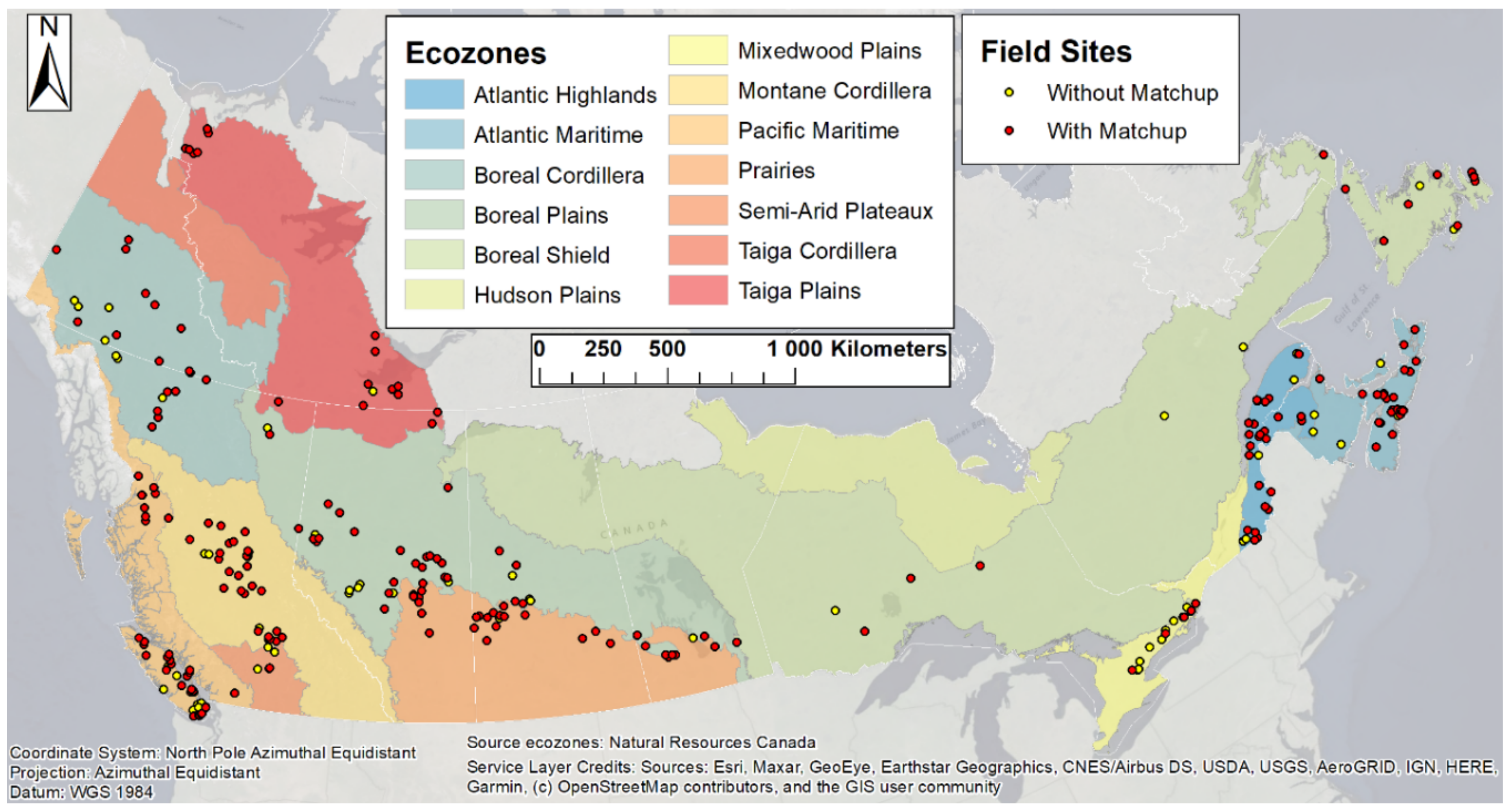
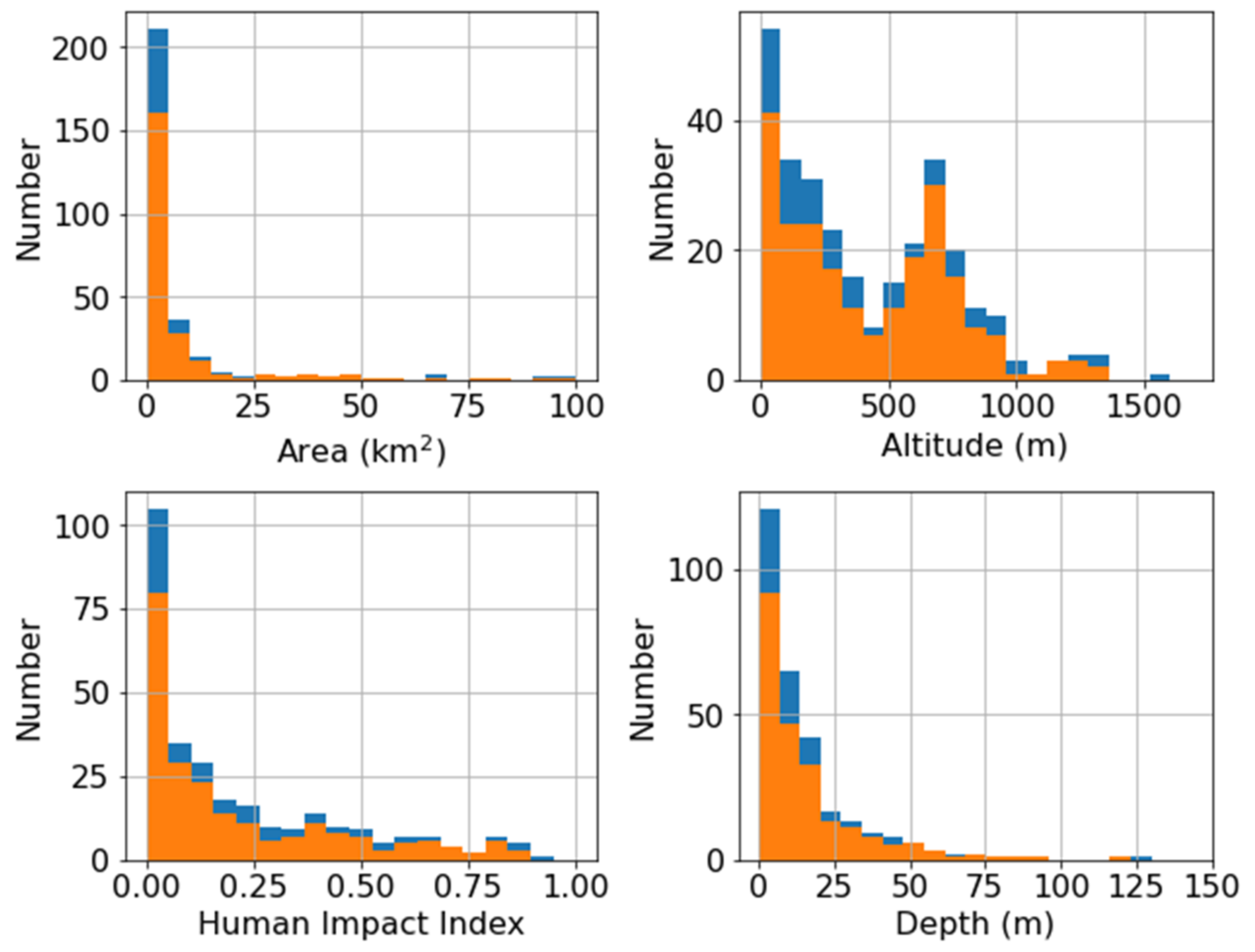
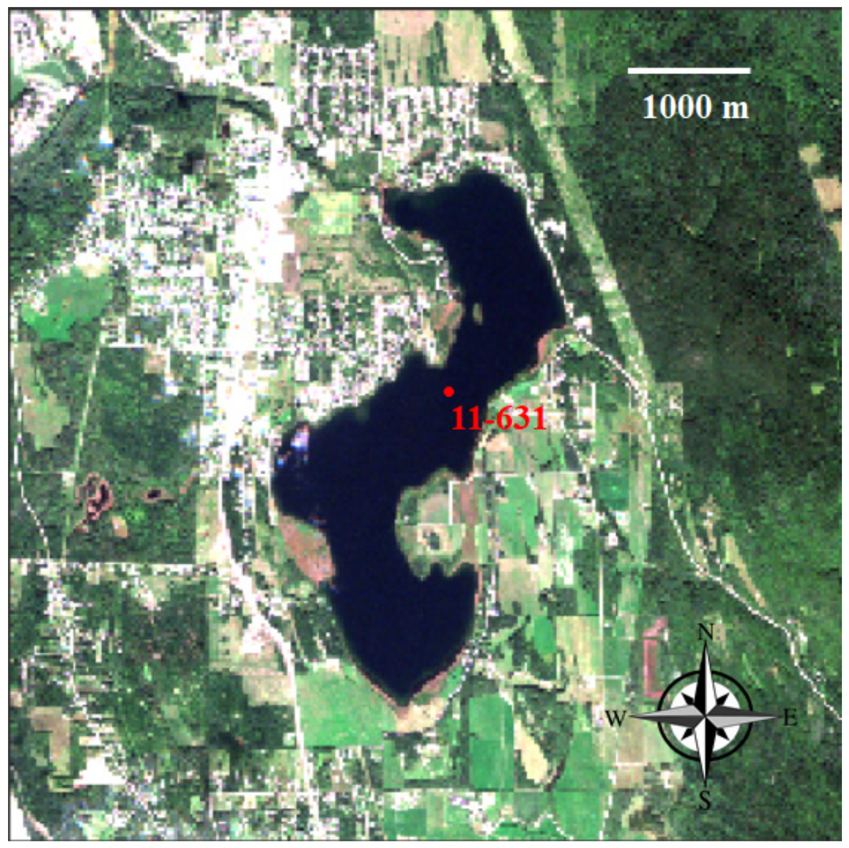
2.1. Study Area
2.2. In Situ Observation Data
2.3. Earth Observation Data
2.4. In Situ Data Processing and Quality Control (QC)
2.4.1. C-OPS
2.4.2. Analytical Spectral Device (ASD)
2.4.3. TriOS-RAMSES
2.4.4. HyperOCR
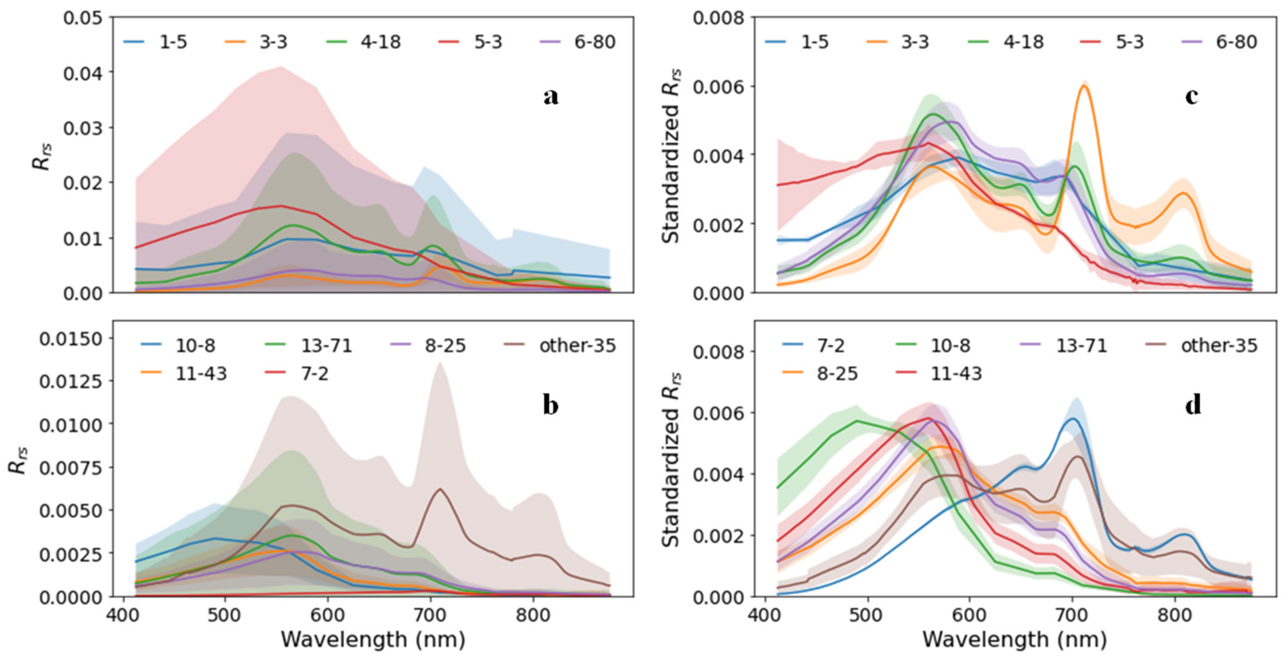
2.4.5. Database of Rrs
2.5. Atmospheric Correction Algorithms and Evaluation
2.5.1. Specific Processing Steps
2.5.2. Preparation of Matchups
2.5.3. Evaluation Metrics
2.6. Radiative Transfer Simulations
- Physical properties of the atmosphere are horizontally homogeneous.
- Land surface are Lambertian and flat.
- Reflectance of the water body is spatially homogeneous.
- Reflectance of the water body includes two parts, the reflectance due to the water-leaving radiance and the water surface reflected diffuse downwelling irradiance.
- No wind over the lake, and the water surface is assumed to be Lambertian.
3. Results
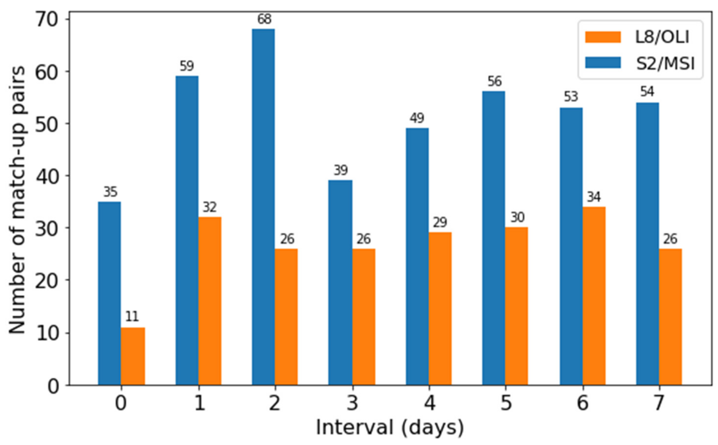
3.1. Number of Valid Matchups
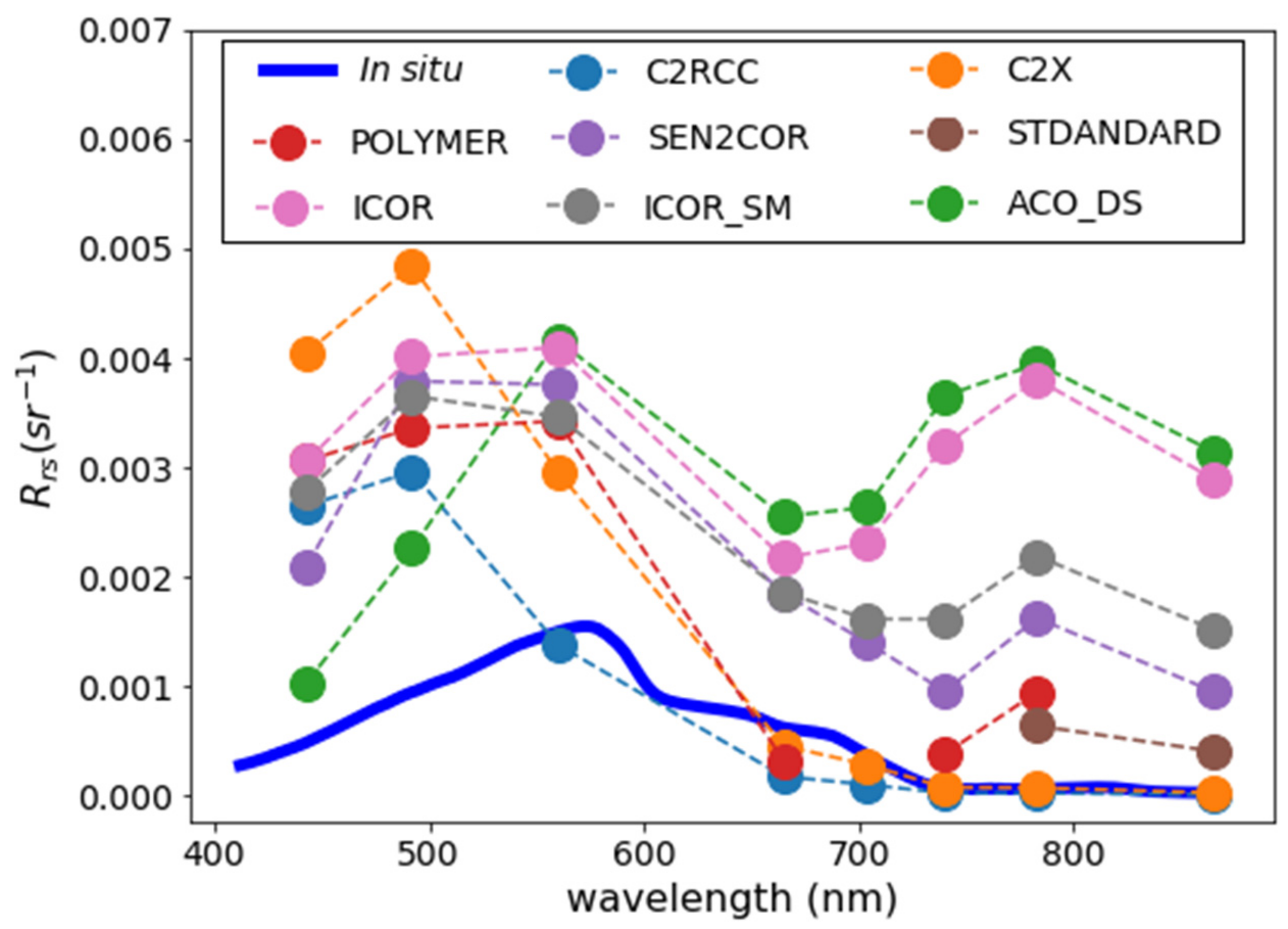
3.2. Validation of Remote Sensing of Reflectance
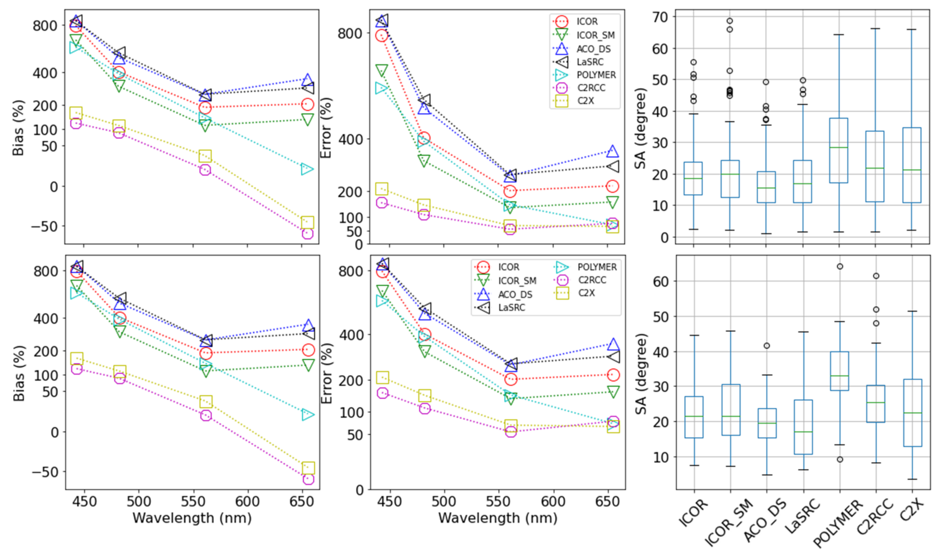
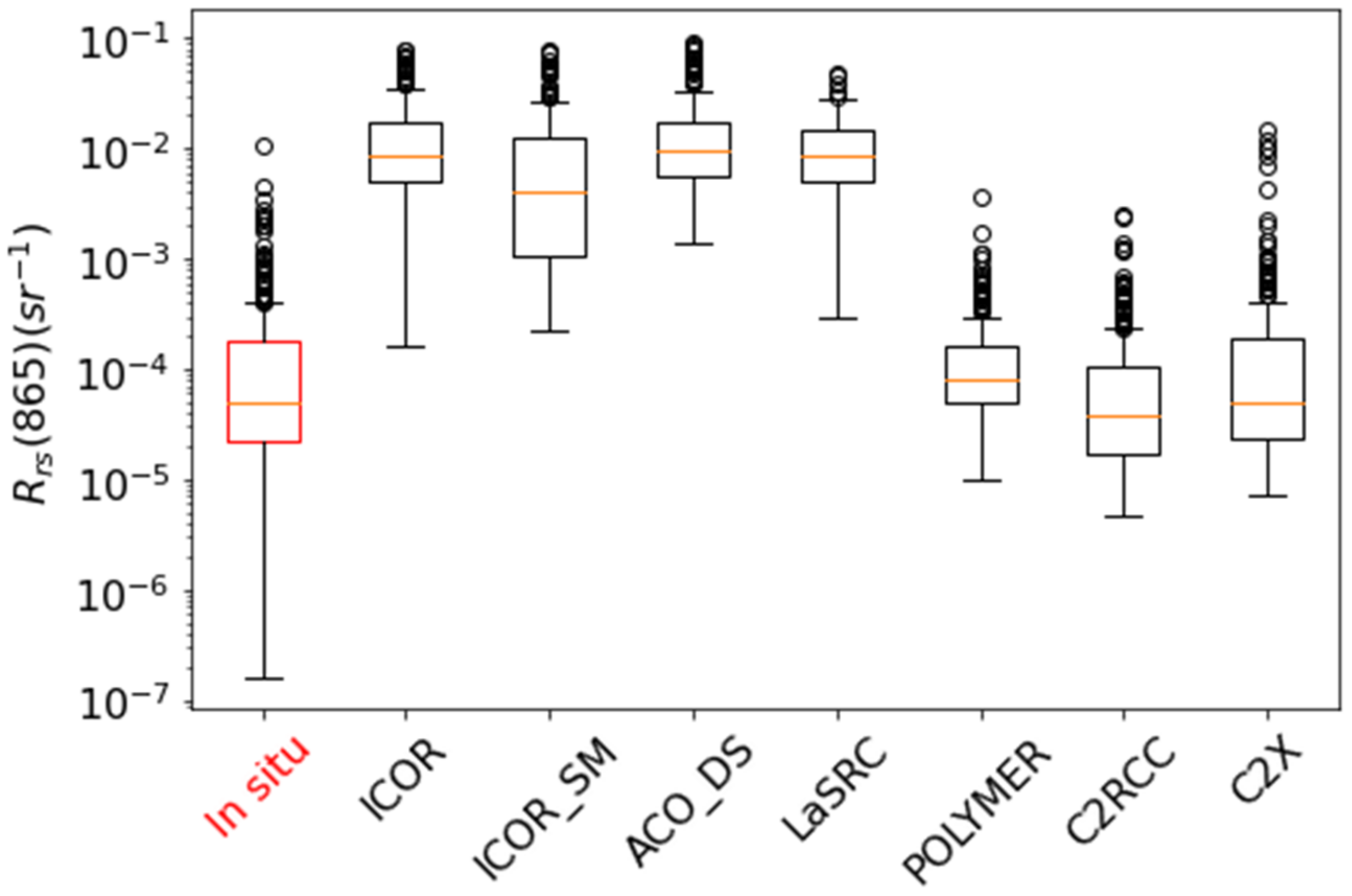
3.2.1. L8/OLI
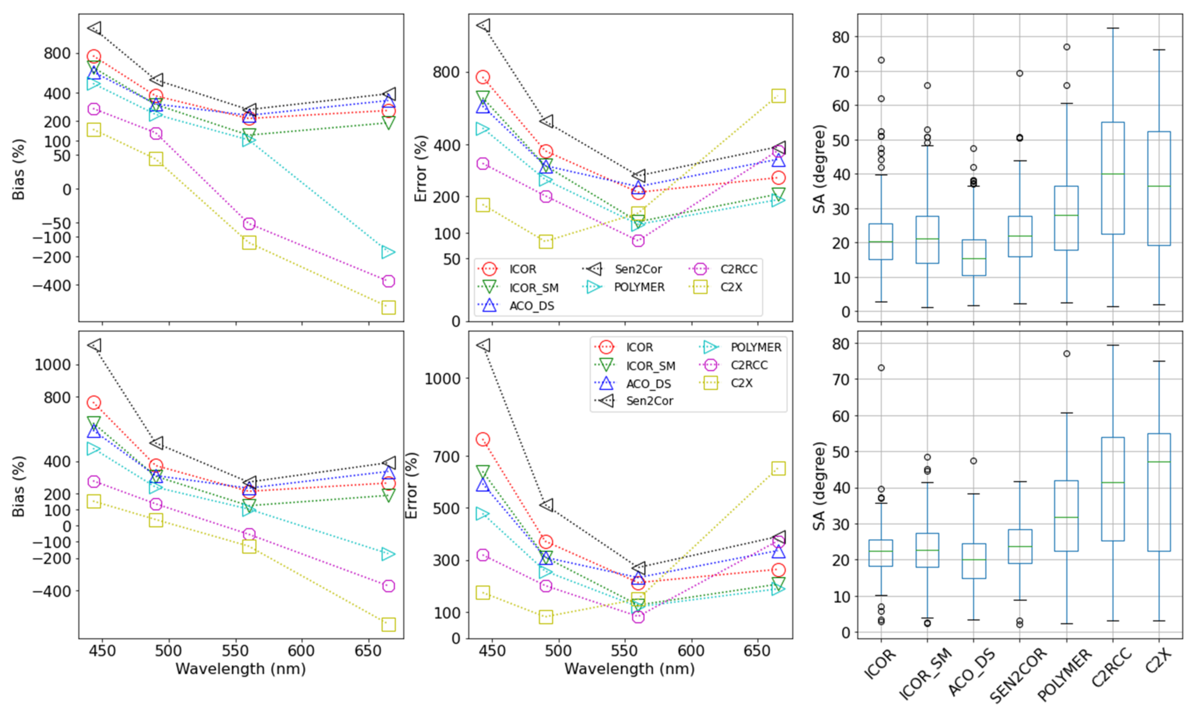
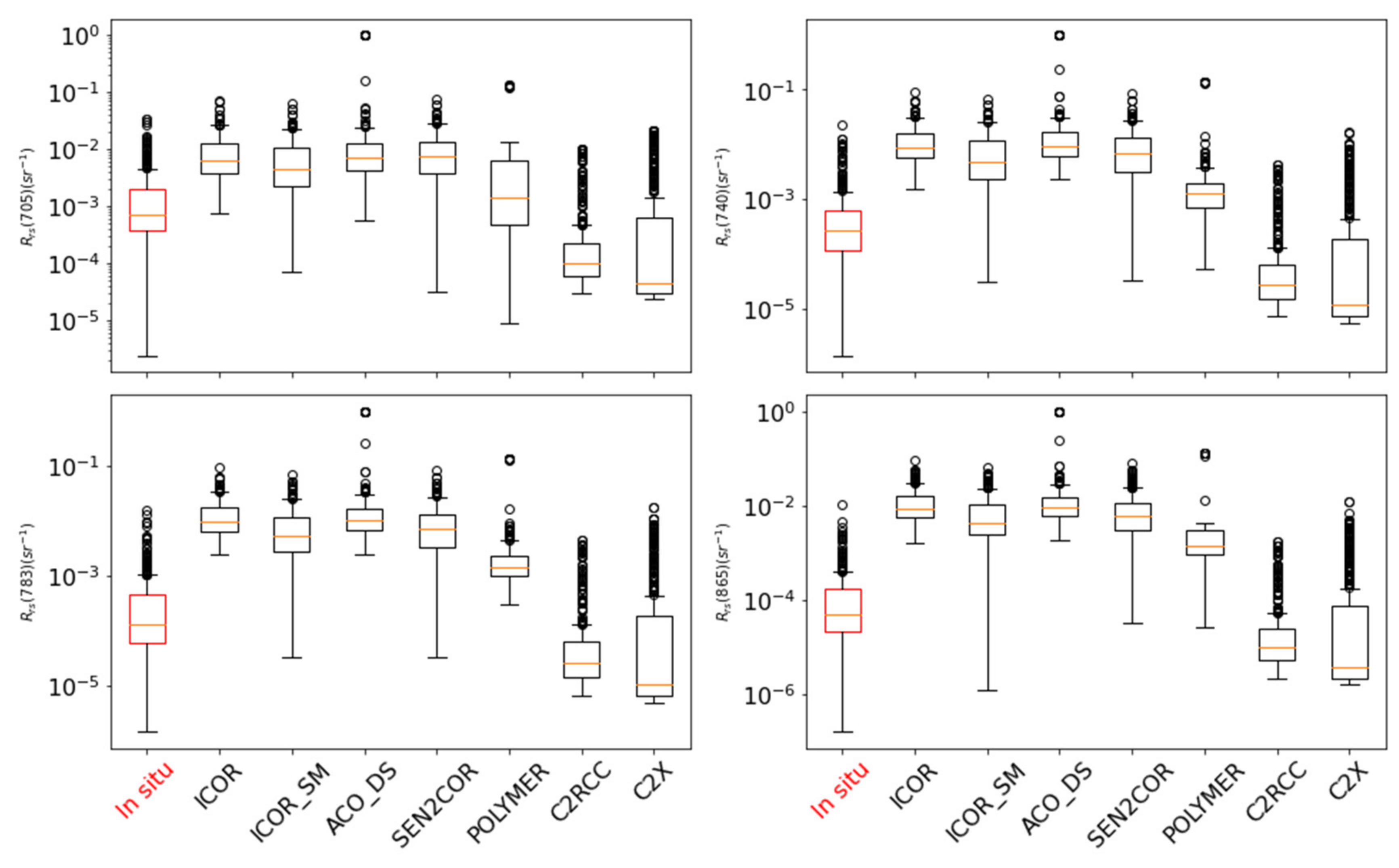
3.2.2. S2/MSI
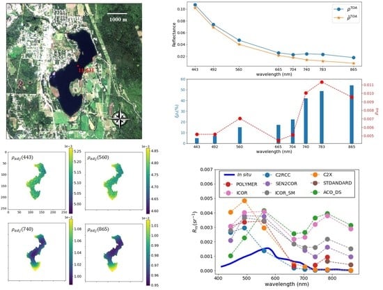
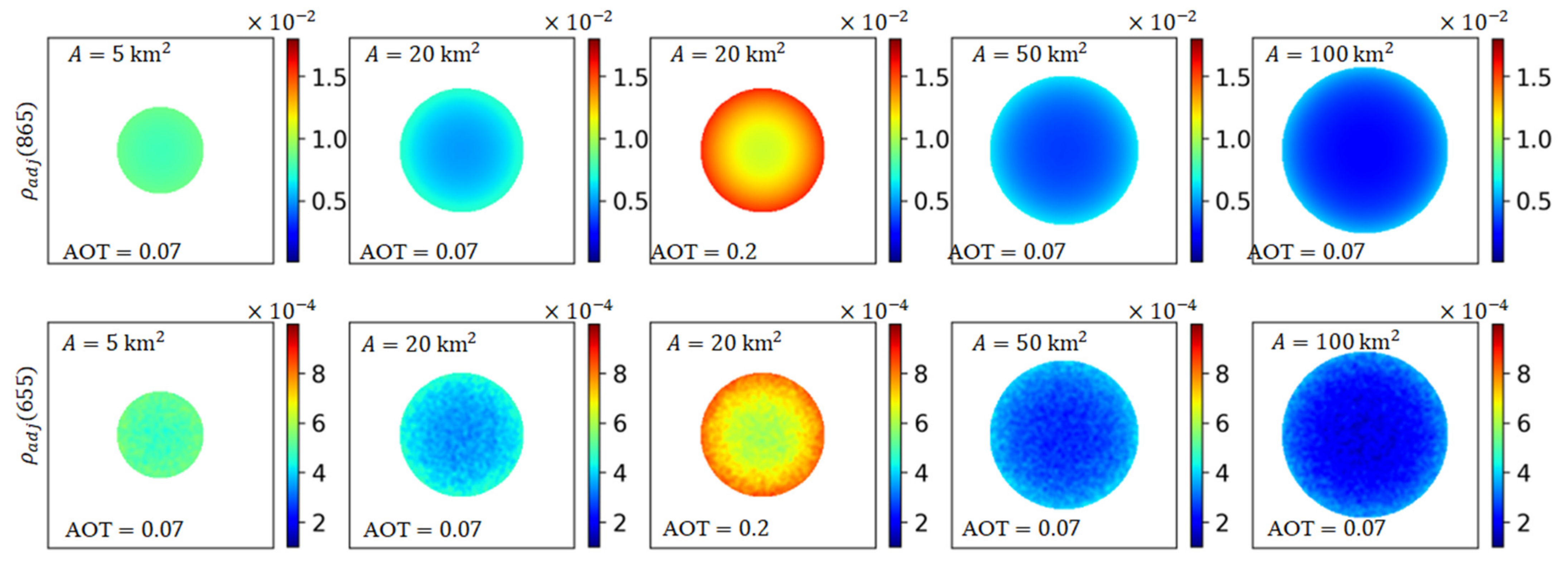
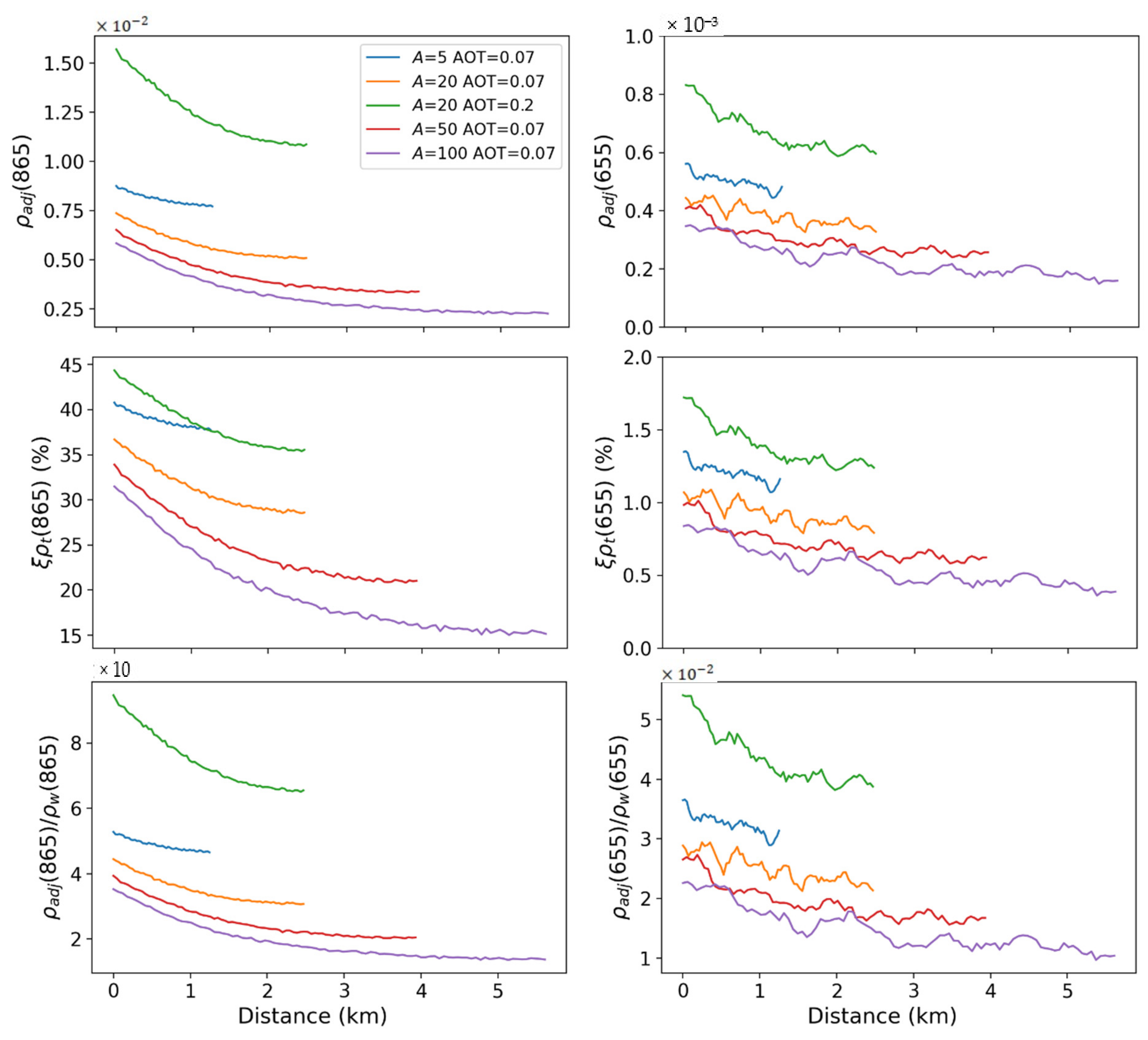
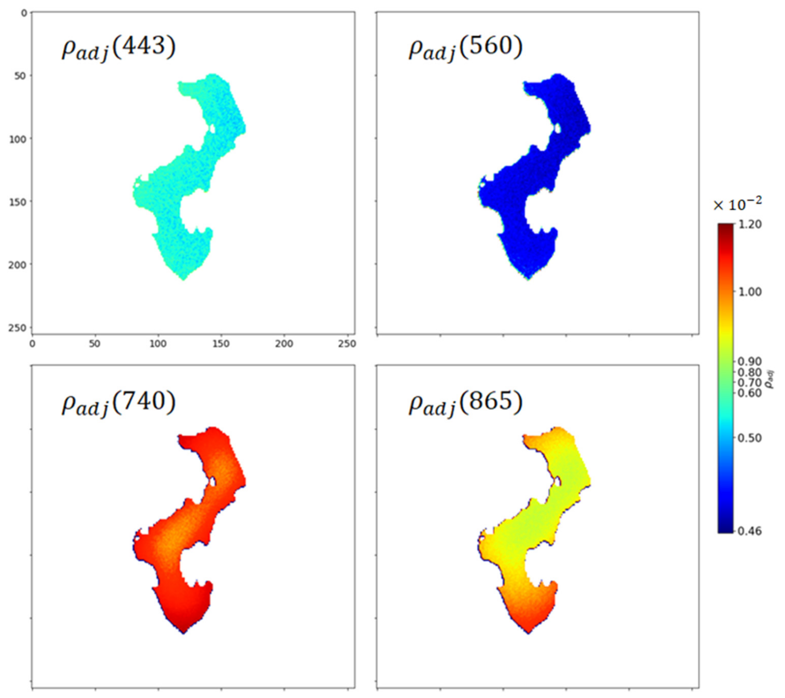
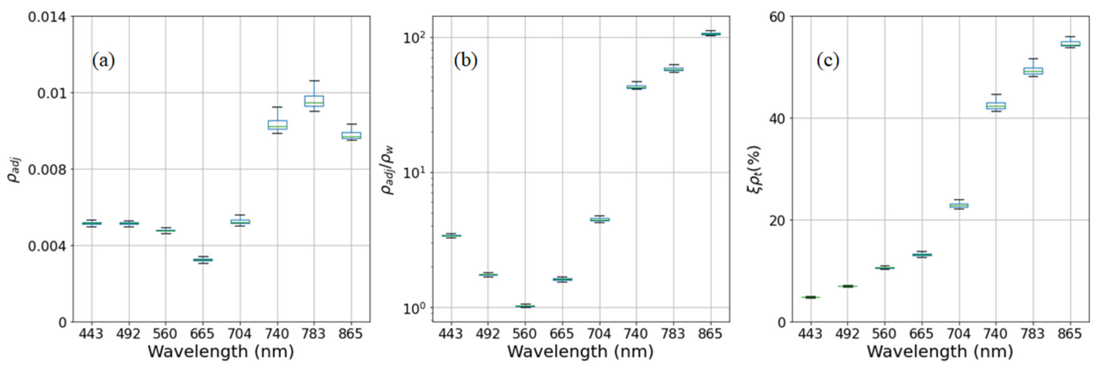
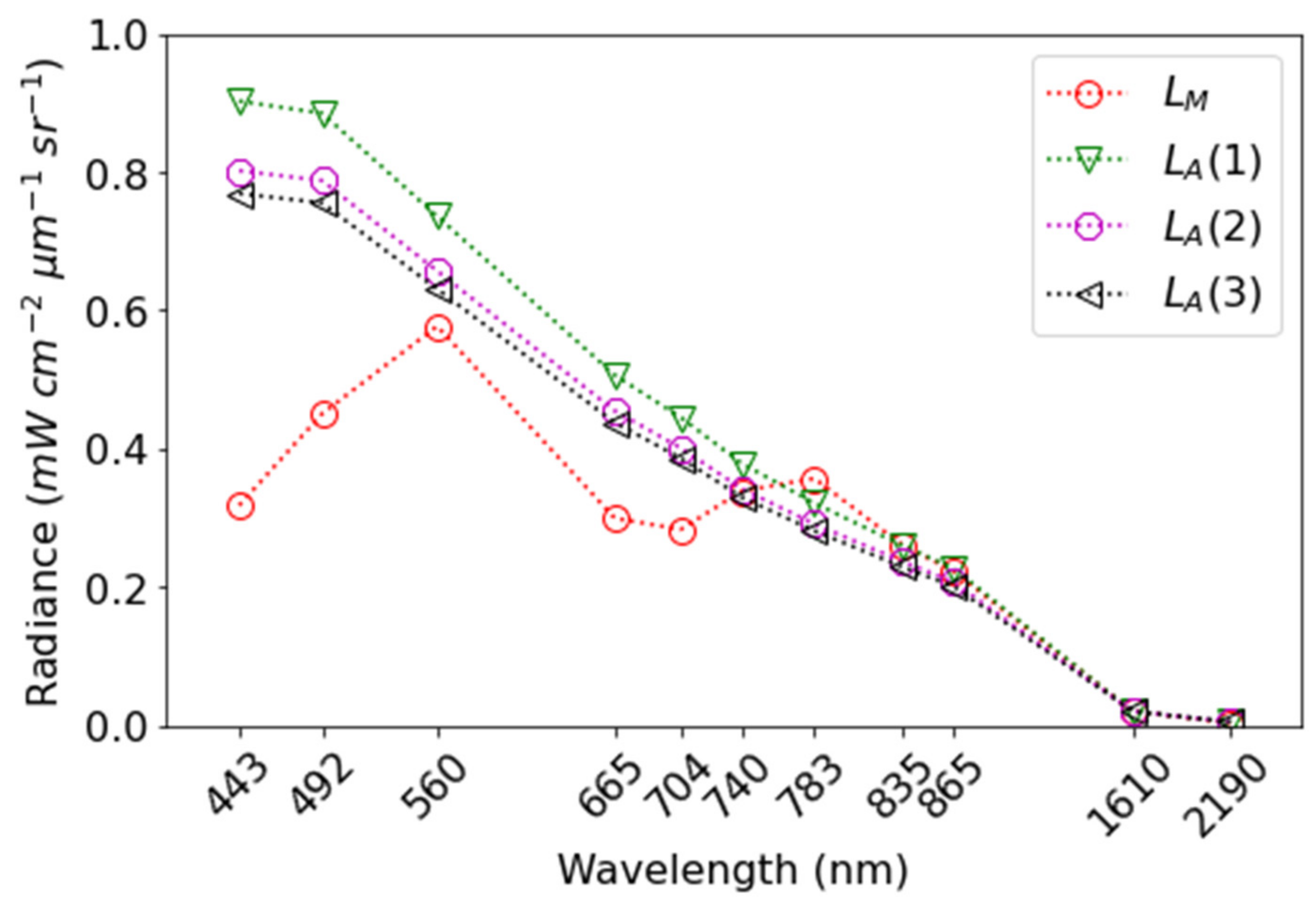
3.3. Simulations of Adjacency Effects
3.3.1. Idealized Case
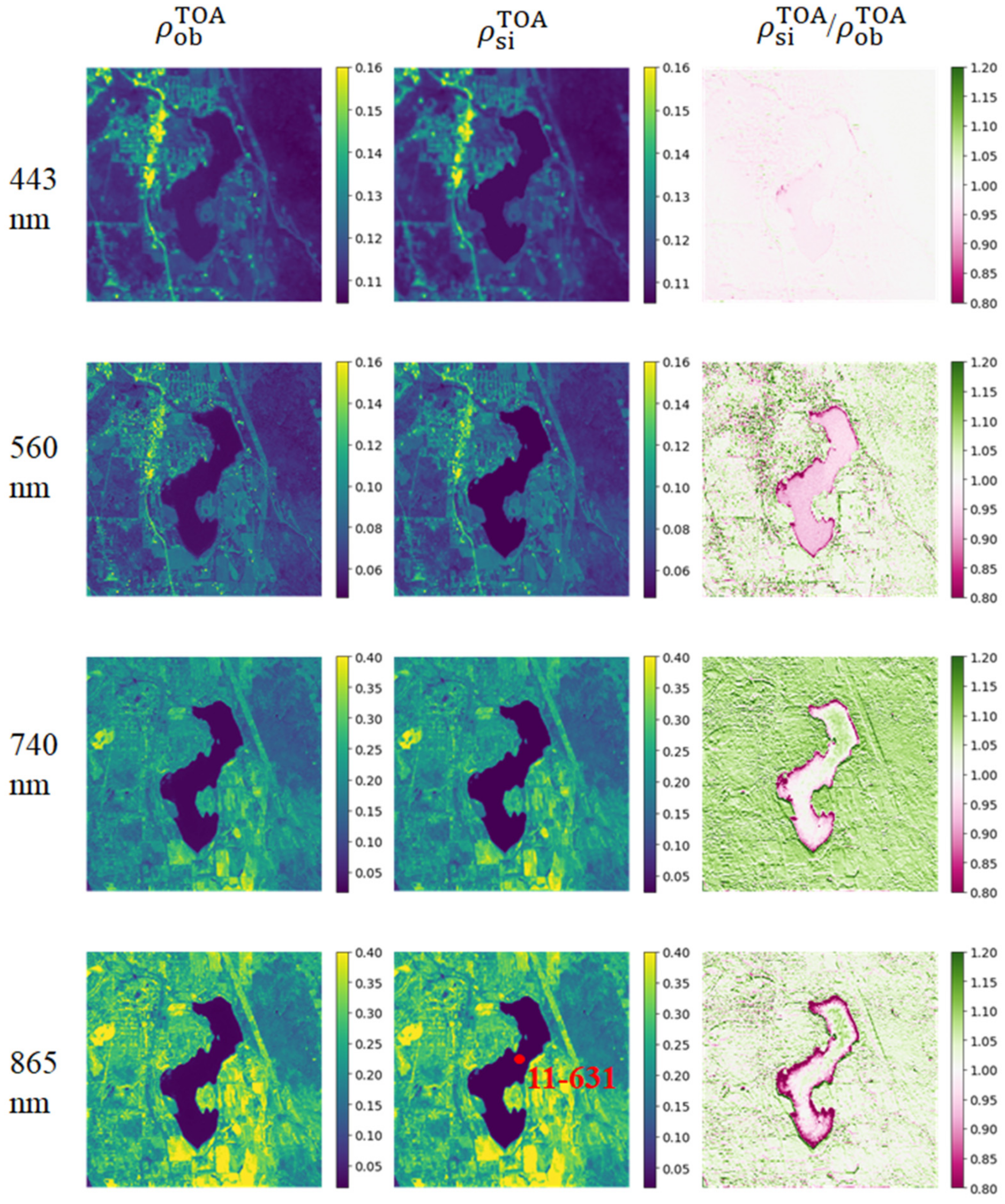
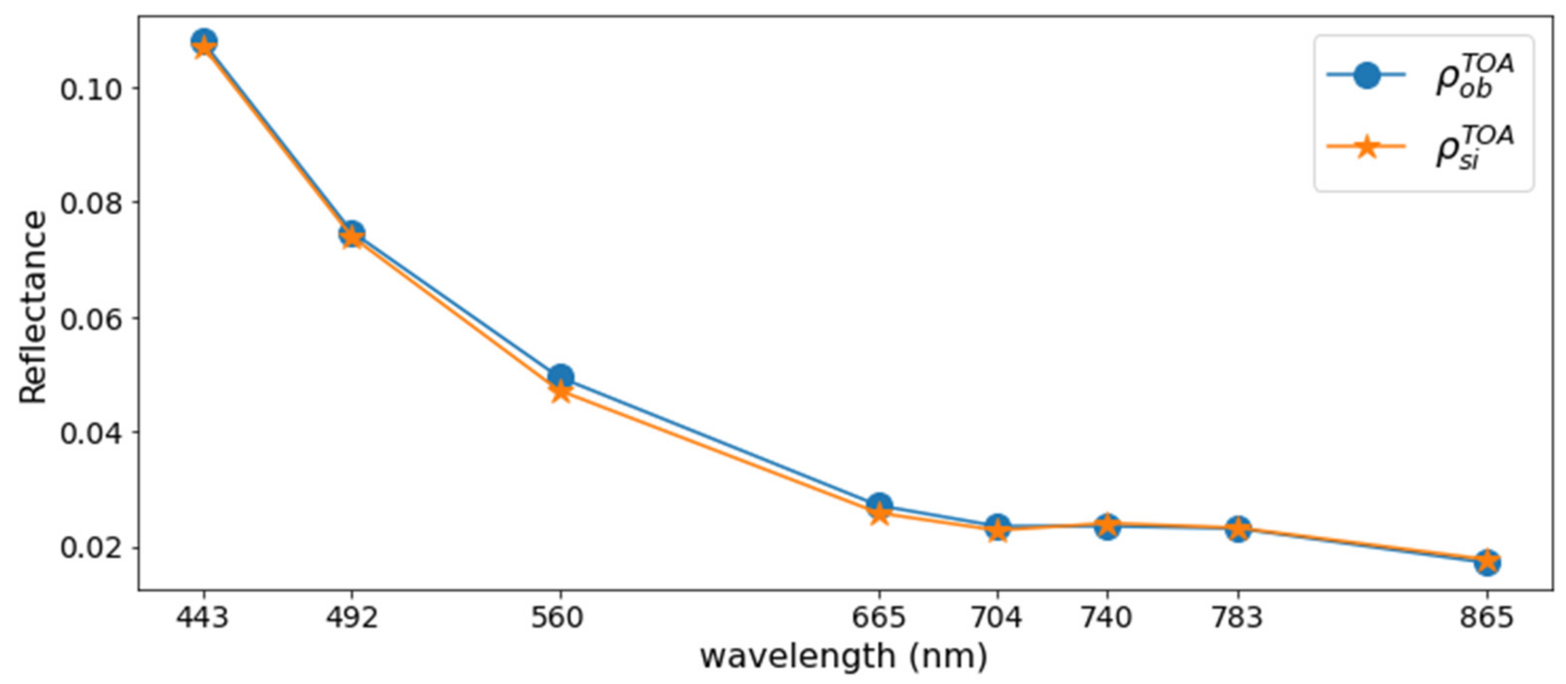
3.3.2. Real Case
4. Discussion
4.1. Sources of Uncertainty
4.2. Adjacency Effects over Small Lakes and Its Influence on Atmospheric Correction
4.3. Potential Method of Improvement
5. Conclusions
Supplementary Materials
Author Contributions
Funding
Data Availability Statement
Acknowledgments
Conflicts of Interest
References
- Dörnhöfer, K.; Oppelt, N. Remote sensing for lake research and monitoring—Recent advances. Ecol. Indic. 2016, 64, 105–122. [Google Scholar] [CrossRef]
- Wrilegy, R.C.; Horne, A.J. Remote sensing and lake eutrophication. Nature 1974, 250, 213–214. [Google Scholar] [CrossRef]
- Brönmark, C.; Hansson, L.A. Environmental issues in lakes and ponds: Current state and perspectives. Environ. Conserv. 2002, 29, 290–307. [Google Scholar] [CrossRef] [Green Version]
- Dudgeon, D.; Arthington, A.H.; Gessner, M.O.; Kawabata, Z.I.; Knowler, D.J.; Lévêque, C.; Naiman, R.J.; Prieur-Richard, A.H.; Soto, D.; Stiassny, M.L.J.; et al. Freshwater biodiversity: Importance, threats, status and conservation challenges. Biol. Rev. Camb. Philos. Soc. 2006, 81, 163–182. [Google Scholar] [CrossRef]
- U.S. Senate. Federal Water Pollution Control Act, 33 U.S.C. 1251 et seq; U.S. Senate: Washington, DC, USA, 2002.
- Government of South Africa. National Water Act; Government of South Africa: Pretoria, South Africa, 1998.
- Australian Government. National Water Management Strategy of Australia and New Zealand; Australian Government: Canberra, Australia, 2000.
- European Commission. Directive 2000/60/EC of the European Parliament and of the Council of 23 October 2000 Establishing a Framework for Community Action in the Field of Water Policy 2000; European Commission: Brussels, Belgium, 2000. [Google Scholar]
- Huot, Y.; Brown, C.A.; Potvin, G.; Antoniades, D.; Baulch, H.M.; Beisner, B.E.; Bélanger, S.; Brazeau, S.; Cabana, H.; Cardille, J.A.; et al. The NSERC Canadian Lake Pulse Network: A national assessment of lake health providing science for water management in a changing climate. Sci. Total Environ. 2019, 695, 133668. [Google Scholar] [CrossRef]
- Topp, S.N.; Pavelsky, T.M.; Jensen, D.; Simard, M.; Ross, M.R.V. Research trends in the use of remote sensing for inland water quality science: Moving towards multidisciplinary applications. Water 2020, 12, 169. [Google Scholar] [CrossRef] [Green Version]
- Scarpace, F.L.; Holmquist, K.W.; Fisher, L.T. Landsat analysis of lake quality. Photogramm. Eng. Remote Sens. 1979, 45, 623–633. [Google Scholar]
- Binding, C.E.; Greenberg, T.A.; Watson, S.B.; Rastin, S.; Gould, J. Long term water clarity changes in North America’s Great Lakes from multi-sensor satellite observations. Limnol. Oceanogr. 2015, 60, 1976–1995. [Google Scholar] [CrossRef]
- Jones, M.O. Application of MODIS for Monitoring Water Quality of a Large Oligotrophic Lake. Graduate Student Thesis, University of Montana, Missoula, MT, USA, 2006. [Google Scholar]
- Cardille, J.A.; Leguet, J.; Giorgio, P.; Cardille, J.A.; Leguet, J.; Remote, G.; Cardille, J.A.; Leguet, J.; Giorgio, P. Remote sensing of lake CDOM using noncontemporaneous field data. Can. J. Remote Sens. 2013, 39, 118–126. [Google Scholar] [CrossRef]
- Brivio, P.A.; Giardino, C.; Zilioli, E. Determination of chlorophyll concentration changes in Lake Garda using an image-based radiative transfer code for Landsat TM images. Int. J. Remote Sens. 2001, 22, 487–502. [Google Scholar] [CrossRef]
- Ungar, S.G.; Pearlman, J.S.; Mendenhall, J.A.; Reuter, D. Overview of the Earth Observing One (EO-1) mission. IEEE Trans. Geosci. Remote Sens. 2003, 41, 1149–1159. [Google Scholar] [CrossRef]
- Zhao, D.; Cai, Y.; Jiang, H.; Xu, D.; Zhang, W.; An, S. Estimation of water clarity in Taihu Lake and surrounding rivers using Landsat imagery. Adv. Water Resour. 2011, 34, 165–173. [Google Scholar] [CrossRef]
- Deutsch, E.S.; Cardille, J.A.; Koll-Egyed, T.; Fortin, M.J. Landsat 8 lake water clarity empirical algorithms: Large-scale calibration and validation using government and citizen science data from across Canada. Remote Sens. 2021, 13, 1257. [Google Scholar] [CrossRef]
- Koll-Egyed, T.; Cardille, J.A.; Deutsch, E. Multiple images improve lake CDOM estimation: Building better landsat 8 empirical algorithms across southern canada. Remote Sens. 2021, 13, 3615. [Google Scholar] [CrossRef]
- Bresciani, M.; Adamo, M.; De Carolis, G.; Matta, E.; Pasquariello, G.; Vaičiute, D.; Giardino, C. Monitoring blooms and surface accumulation of cyanobacteria in the Curonian Lagoon by combining MERIS and ASAR data. Remote Sens. Environ. 2014, 146, 124–135. [Google Scholar] [CrossRef]
- Chen, J.; Quan, W. Using Landsat/TM imagery to estimate nitrogen and phosphorus concentration in Taihu Lake, China. IEEE J. Sel. Top. Appl. Earth Obs. Remote Sens. 2012, 5, 273–280. [Google Scholar] [CrossRef]
- Kloiber, S.M.; Brezonik, P.L.; Bauer, M.E. Application of Landsat imagery to regional-scale assessments of lake clarity. Water Res. 2002, 36, 4330–4340. [Google Scholar] [CrossRef]
- Kloiber, S.M.; Brezonik, P.L.; Olmanson, L.G.; Bauer, M.E. A procedure for regional lake water clarity assessment using Landsat multispectral data. Remote Sens. Environ. 2002, 82, 38–47. [Google Scholar] [CrossRef]
- Lathrop, R.G. Landsat Thematic Mapper monitoring of turbid inland water quality. Photogramm. Eng. Remote Sens. 1992, 58, 465–470. [Google Scholar]
- Lillesand, T.M.; Johnson, W.L.; Deuell, R.L. Use of landsat data to predict the trophic state of Minnesota lakes. Photogramm. Eng. Remote Sens. 1983, 49, 219–229. [Google Scholar]
- Ma, R.; Duan, H.; Gu, X.; Zhang, S. Detecting aquatic vegetation changes in Taihu lake, China using multi-temporal satellite imagery. Sensors 2008, 8, 3988–4005. [Google Scholar] [CrossRef] [PubMed] [Green Version]
- Menken, K.D.; Brezonik, P.L.; Bauer, M.E. Influence of chlorophyll and colored dissolved organic matter (CDOM) on lake reflectance spectra: Implications for measuring lake properties by remote sensing. Lake Reserv. Manag. 2006, 22, 179–190. [Google Scholar] [CrossRef] [Green Version]
- Franz, B.A.; Bailey, S.W.; Kuring, N.; Werdell, P.J. Ocean Color Measurements from Landsat-8 OLI using SeaDAS. Proc. Ocean Opt. 2014, 12, 26–31. [Google Scholar]
- Antoine, D.; Morel, A. A multiple scattering algorithm for atmospheric correction of remotely sensed ocean colour (MERIS instrument): Principle and implementation for atmospheres carrying various aerosols including absorbing ones. Int. J. Remote Sens. 1999, 20, 1875–1916. [Google Scholar] [CrossRef]
- Gordon, H.R.; Castaho, D.J. Coastal Zone Color Scanner atmospheric correction algorithm: Multiple scattering effects. Appl. Opt. 1987, 26, 2111–2122. [Google Scholar] [CrossRef]
- Mobley, C.D.; Werdell, J.; Franz, B.; Ahmad, Z.; Bailey, S. Atmospheric Correction for Satellite Ocean Color Radiometry; A Tutorial and Documentation of the Algorithms Used by the NASA Ocean Biology Processing Group; National Aeronautics and Space Administration: Greenbelt, MD, USA, 2016; pp. 1–73. [Google Scholar]
- McClain, C.R.; Hooker, S.; Feldman, G.; Bontempi, P. Satellite data for ocean biology, biogeochemistry, and climate research. Eos 2006, 87, 340–342. [Google Scholar] [CrossRef]
- Mouw, C.B.; Greb, S.; Aurin, D.; Digiacomo, P.M.; Lee, Z.; Twardowski, M.; Binding, C.; Hu, C.; Ma, R.; Moore, T.; et al. Remote Sensing of Environment Aquatic color radiometry remote sensing of coastal and inland waters: Challenges and recommendations for future satellite missions. Remote Sens. Environ. 2015, 160, 15–30. [Google Scholar] [CrossRef]
- Pahlevan, N.; Mangin, A.; Balasubramanian, S.V.; Smith, B.; Alikas, K.; Arai, K.; Barbosa, C.; Bélanger, S.; Binding, C.; Bresciani, M.; et al. ACIX-Aqua: A global assessment of atmospheric correction methods for Landsat-8 and Sentinel-2 over lakes, rivers, and coastal waters. Remote Sens. Environ. 2021, 258, 112366. [Google Scholar] [CrossRef]
- Warren, M.A.; Simis, S.G.H.; Martinez-Vicente, V.; Poser, K.; Bresciani, M.; Alikas, K.; Spyrakos, E.; Giardino, C.; Ansper, A. Assessment of atmospheric correction algorithms for the Sentinel-2A MultiSpectral Imager over coastal and inland waters. Remote Sens. Environ. 2019, 225, 267–289. [Google Scholar] [CrossRef]
- Pereira-Sandoval, M.; Ruescas, A.; Urrego, P.; Ruiz-Verdú, A.; Delegido, J.; Tenjo, C.; Soria-Perpinyà, X.; Vicente, E.; Soria, J.; Moreno, J. Evaluation of atmospheric correction algorithms over spanish inland waters for sentinel-2 multi spectral imagery data. Remote Sens. 2019, 11, 1469. [Google Scholar] [CrossRef] [Green Version]
- Doerffer, R.; Schiller, H. The MERIS case 2 water algorithm. Int. J. Remote Sens. 2007, 28, 517–535. [Google Scholar] [CrossRef]
- Brockmann, C.; Doerffer, R.; Peters, M.; Stelzer, K.; Embacher, S.; Ruescas, A. Evolution of the C2RSS Neural Network for Sentinel 2 and 3 for the Ritreval of Ocean Color Products in Normal and Extreme Optically Complex Waters. In Proceedings of the Living Planet Symposium 2016, Prague, Czech Republic, 9–13 May 2016. [Google Scholar]
- Steinmetz, F.; Deschamps, P.-Y.; Ramon, D. (POLYMER)Atmospheric correction in presence of sun glint: Application to MERIS. Opt. Express 2011, 19, 9783–9800. [Google Scholar] [CrossRef] [PubMed] [Green Version]
- Vanhellemont, Q.; Ruddick, K. Atmospheric correction of metre-scale optical satellite data for inland and coastal water applications. Remote Sens. Environ. 2018, 216, 586–597. [Google Scholar] [CrossRef]
- De Keukelaere, L.; Sterckx, S.; Adriaensen, S.; Knaeps, E.; Reusen, I.; Giardino, C.; Bresciani, M.; Hunter, P.; Neil, C.; Van Der Zande, D.; et al. Atmospheric correction of Landsat-8/OLI and Sentinel-2/MSI data using iCOR algorithm: Validation for coastal and inland waters. Eur. J. Remote Sens. 2018, 51, 525–542. [Google Scholar] [CrossRef] [Green Version]
- Main-Knorn, M.; Pflug, B.; Louis, J.; Debaecker, V.; Müller-Wilm, U.; Gascon, F. Sen2Cor for Sentinel-2. In Image and Signal Processing for Remote Sensing; SPIE: Bellingham, WA, USA, 2017; p. 3. [Google Scholar]
- Otterman, J.; Fraser, R.S. Adjacency effects on imaging by surface reflection and atmospheric scattering: Cross radiance to zenith. Appl. Opt. 1979, 18, 2852. [Google Scholar] [CrossRef] [PubMed]
- Santer, R.; Schmechtig, C. Adjacency effects on water surfaces: Primary scattering approximation and sensitivity study. Appl. Opt. 2000, 39, 361. [Google Scholar] [CrossRef] [PubMed]
- Tanré, D.; Herman, M.; Deschamps, P.Y. Influence of the background contribution upon space measurements of ground reflectance. Appl. Opt. 1981, 20, 3676. [Google Scholar] [CrossRef]
- Tanré, D.; Deschamps, P.Y.; Duhaut, P.; Herman, M. Adjacency effect produced by the atmospheric scattering in thematic mapper data. J. Geophys. Res. 1987, 92, 12000–12006. [Google Scholar] [CrossRef]
- Kiselev, V.; Bulgarelli, B.; Heege, T. Sensor independent adjacency correction algorithm for coastal and inland water systems. Remote Sens. Environ. 2015, 157, 85–95. [Google Scholar] [CrossRef]
- Reinersman, P.N.; Carder, K.L. Monte Carlo simulation of the atmospheric point-spread function with an application to correction for the adjacency effect. Appl. Opt. 1995, 34, 4453. [Google Scholar] [CrossRef]
- Sterckx, S.; Knaeps, S.; Kratzer, S.; Ruddick, K. SIMilarity Environment Correction (SIMEC) applied to MERIS data over inland and coastal waters. Remote Sens. Environ. 2015, 157, 96–110. [Google Scholar] [CrossRef]
- Bulgarelli, B.; Kiselev, V.; Zibordi, G. Simulation and analysis of adjacency effects in coastal waters: A case study. Appl. Opt. 2014, 53, 1523–1545. [Google Scholar] [CrossRef] [PubMed]
- Bulgarelli, B.; Zibordi, G. On the detectability of adjacency effects in ocean color remote sensing of mid-latitude coastal environments by SeaWiFS, MODIS-A, MERIS, OLCI, OLI and MSI. Remote Sens. Environ. 2018, 209, 423–438. [Google Scholar] [CrossRef]
- Bulgarelli, B. Seasonal Impact of Adjacency Effects on Ocean Color Radiometry at the AAOT Validation Site. IEEE Geosci. Remote Sens. Lett. 2018, 15, 488–492. [Google Scholar] [CrossRef]
- Richter, R. A fast atmospheric correction algorithm applied to landsat tm images. Int. J. Remote Sens. 1990, 11, 159–166. [Google Scholar] [CrossRef]
- Minomura, M.; Kuze, H.; Takeuchi, N. Adjacency effect in the atmospheric correction of satellite remote sensing data: Evaluation of the influence of aerosol extinction profiles. Opt. Rev. 2001, 8, 133–141. [Google Scholar] [CrossRef]
- Mousivand, A.; Verhoef, W.; Menenti, M.; Gorte, B. Modeling Top of Atmosphere Radiance over Heterogeneous Non-Lambertian Rugged Terrain. Remote Sens. 2015, 7, 8019–8044. [Google Scholar] [CrossRef] [Green Version]
- Bulgarelli, B.; Zibordi, G. Adjacency radiance around a small island: Implications for system vicarious calibrations. Appl. Opt. 2020, 59, C63. [Google Scholar] [CrossRef]
- Kuhn, C.; Matos, A.; De Ward, N.; Loken, L.; Oliveira, H.; Kampel, M.; Richey, J.; Stadler, P.; Crawford, J.; Striegl, R.; et al. Performance of Landsat-8 and Sentinel-2 surface reflectance products for river remote sensing retrievals of chlorophylla and turbidity. Remote Sens. Environ. 2019, 224, 104–118. [Google Scholar] [CrossRef] [Green Version]
- Sun, B.; Schäfer, M.; Ehrlich, A.; Jäkel, E.; Wendisch, M. Influence of atmospheric adjacency effect on top-of-atmosphere radiances and its correction in the retrieval of Lambertian surface reflectivity based on three-dimensional radiative transfer. Remote Sens. Environ. 2021, 263, 112543. [Google Scholar] [CrossRef]
- Statistics Canada. Ecological Land Classification, 2017; Statistics Canada: Ottava, ON, Canada, 2018; ISBN 9780660245010.
- McColl, R.W. Encyclopedia of World Geography; Infobase Publishing: New York, NY, USA, 2015; ISBN 978-0-8160-5786-3. [Google Scholar]
- Morrow, J.H.; Booth, C.R.; Lind, R.N.; Hooker, S.B.; Profiling, O.; In, S.C.; Hooker, S.B.; Booth, C.R. The Compact-Optical Profiling System (C-OPS). In Advances in Measuring the Apparent Optical Properties (AOPs) of Optically Complex Waters, NASA Tech.Memo; Biospherical Instruments Inc: 2010–215856; NASA Goddard Space Flight Center: Greenbelt, MD, USA, 2010; pp. 42–50. [Google Scholar]
- Ruddick, K.G.; Voss, K.; Banks, A.C.; Boss, E.; Castagna, A.; Frouin, R.; Hieronymi, M.; Jamet, C.; Johnson, B.C.; Kuusk, J.; et al. A Review of Protocols for Fiducial Reference Measurements of Downwelling Irradiance for the Validation of Satellite Remote Sensing Data over Water. Remote Sens. 2019, 11, 1742. [Google Scholar] [CrossRef] [Green Version]
- Spyrakos, E.; O’Donnell, R.; Hunter, P.D.; Miller, C.; Scott, M.; Simis, S.G.H.; Neil, C.; Barbosa, C.C.F.; Binding, C.E.; Bradt, S.; et al. Optical types of inland and coastal waters. Limnol. Oceanogr. 2018, 63, 846–870. [Google Scholar] [CrossRef] [Green Version]
- Franz, B.A.; Bailey, S.W.; Kuring, N.; Werdell, P.J. Ocean color measurements with the Operational Land Imager on Landsat-8: Implementation and evaluation in SeaDAS. J. Appl. Remote Sens. 2015, 9, 096070. [Google Scholar] [CrossRef]
- Pahlevan, N.; Sarkar, S.; Franz, B.A.; Balasubramanian, S.V.; He, J. Sentinel-2 MultiSpectral Instrument (MSI) data processing for aquatic science applications: Demonstrations and validations. Remote Sens. Environ. 2017, 201, 47–56. [Google Scholar] [CrossRef]
- Hooker, S.B.; Morrow, J.H.; Matsuoka, A. Apparent optical properties of the Canadian Beaufort Sea—Part 2: The 1% and 1 cm perspective in deriving and validating AOP data products. Biogeosciences 2013, 10, 4511–4527. [Google Scholar] [CrossRef] [Green Version]
- Morel, A.; Gentili, B. Diffuse reflectance of oceanic waters II Bidirectional aspects. Appl. Opt. 1993, 32, 6864. [Google Scholar] [CrossRef] [PubMed]
- Mueller, J.L.; Austin, R.W.; Morel, A.Y.; Fargion, G.S.; McClain, C.R. Ocean Optics Protocols for Satellite Ocean Color Sensor Validation, Revision 4, Volume I: Introduction, Background and Conventions; Nasa/Tm-2003-21621; NASA Goddard Space Flight Center: Greenbelt, MD, USA, 2003; Volume I, p. 56. [Google Scholar]
- Morel, A.; Maritorena, S. Bio-optical properties of oceanic waters: A reappraisal. J. Geophys. Res. Ocean. 2001, 106, 7163–7180. [Google Scholar] [CrossRef] [Green Version]
- Mobley, C.D. Estimation of the remote-sensing reflectance from above-surface measurements. Appl. Opt. 1999, 38, 7442–7455. [Google Scholar] [CrossRef]
- Ruddick, K.G.; De Cauwer, V.; Park, Y.J.; Moore, G. Seaborne measurements of near infrared water-leaving reflectance: The similarity spectrum for turbid waters. Limnol. Oceanogr. 2006, 51, 1167–1179. [Google Scholar] [CrossRef] [Green Version]
- Simis, S.G.H.; Olsson, J. Unattended processing of shipborne hyperspectral reflectance measurements. Remote Sens. Environ. 2013, 135, 202–212. [Google Scholar] [CrossRef] [Green Version]
- Kutser, T.; Vahtmäe, E.; Paavel, B.; Kauer, T. Removing glint effects from field radiometry data measured in optically complex coastal and inland waters. Remote Sens. Environ. 2013, 133, 85–89. [Google Scholar] [CrossRef]
- Jiang, D.; Matsushita, B.; Yang, W. A simple and effective method for removing residual reflected skylight in above-water remote sensing reflectance measurements. ISPRS J. Photogramm. Remote Sens. 2020, 165, 16–27. [Google Scholar] [CrossRef]
- Lee, Z.; Carder, K.L.; Arnone, R.A. (QAA)Deriving Inherent Optical Properties from Water Color: A Multiband Quasi-Analytical Algorithm for Optically Deep Waters. Appl. Opt. 2002, 41, 5755. [Google Scholar] [CrossRef] [PubMed]
- Bailey, S.W.; Franz, B.A.; Werdell, P.J. Estimation of near-infrared water-leaving reflectance for satellite ocean color data processing. Opt. Express 2010, 18, 7521–7527. [Google Scholar] [CrossRef] [PubMed]
- Siegel, D.A.; Wang, M.; Maritorena, S.; Robinson, W. Atmospheric correction of satellite ocean color imagery: The black pixel assumption. Appl. Opt. 2000, 39, 3582–3591. [Google Scholar] [CrossRef] [PubMed]
- Wang, M.; Shi, W.; Son, S. Evaluation of MODIS SWIR and NIR-SWIR atmospheric correction algorithms using SeaBASS data. Remote Sens. Environ. 2009, 113, 635–644. [Google Scholar] [CrossRef]
- Vanhellemont, Q. Adaptation of the dark spectrum fitting atmospheric correction for aquatic applications of the Landsat and Sentinel-2 archives. Remote Sens. Environ. 2019, 225, 175–192. [Google Scholar] [CrossRef]
- U.S. Geological Survey. Landsat 8 Surface Reflectance Code (LASRC) Poduct Guide; No. LSDS-1368 Version 2.0; U.S. Geological Survey: Reston, VA, USA, 2019; p. 40.
- Mayer, B.; Kylling, A. Technical note: The libRadtran software package for radiative transfer calculations—Description and examples of use. Atmos. Chem. Phys. 2006, 5, 1855–1877. [Google Scholar] [CrossRef] [Green Version]
- Richter, R.; Schlapfer, D. Atmospheric and topographic correction (ATCOR theoretical background document). DLR IB 2020, 1, 0564-03. [Google Scholar]
- Sterckx, S.; Knaeps, E.; Adriaensen, S.; Reusen, I.; De Keukelaere, L.; Hunter, P.; Giardino, C.; Odermatt, D. Opera: An atmospheric correction for land and water. Proc. Sentin. Sci. Work. 2015, 1, 3–6. [Google Scholar]
- Guanter, L. New Algorithms for Atmospheric Correction and Retrieval of Biophysical Parameters in Earth Observation. Application to ENVISAT/MERIS Data; Universitat de Valencia: Valencia, Spain, 2006. [Google Scholar]
- Olmanson, L.G.; Bauer, M.E.; Brezonik, P.L. A 20-year Landsat water clarity census of Minnesota’s 10,000 lakes. Remote Sens. Environ. 2008, 112, 4086–4097. [Google Scholar] [CrossRef]
- Sriwongsitanon, N.; Surakit, K.; Thianpopirug, S. Influence of atmospheric correction and number of sampling points on the accuracy of water clarity assessment using remote sensing application. J. Hydrol. 2011, 401, 203–220. [Google Scholar] [CrossRef]
- Tebbs, E.J.; Remedios, J.J.; Harper, D.M. Remote sensing of chlorophyll-a as a measure of cyanobacterial biomass in Lake Bogoria, a hypertrophic, saline-alkaline, flamingo lake, using Landsat ETM+. Remote Sens. Environ. 2013, 135, 92–106. [Google Scholar] [CrossRef]
- Ahmad, Z.; Franz, B.A.; McClain, C.R.; Kwiatkowska, E.J.; Werdell, J.; Shettle, E.P.; Holben, B.N. New aerosol models for the retrieval of aerosol optical thickness and normalized water-leaving radiances from the SeaWiFS and MODIS sensors over coastal regions and open oceans. Appl. Opt. 2010, 49, 5545–5560. [Google Scholar] [CrossRef]
- Kavzoglu, T. Simulating Landsat ETM+ imagery using DAIS 7915 hyperspectral scanner data. Int. J. Remote Sens. 2004, 25, 5049–5067. [Google Scholar] [CrossRef]
- Doxani, G.; Vermote, E.; Roger, J.C.; Gascon, F.; Adriaensen, S.; Frantz, D.; Hagolle, O.; Hollstein, A.; Kirches, G.; Li, F.; et al. Atmospheric correction inter-comparison exercise. Remote Sens. 2018, 10, 352. [Google Scholar] [CrossRef] [Green Version]
- Bulgarelli, B.; Zibordi, G.; Mélin, F. On the minimization of adjacency effects in SeaWiFS primary data products from coastal areas. Opt. Express 2018, 26, 301–313. [Google Scholar] [CrossRef]
- Bulgarelli, B.; Kiselev, V.; Zibordi, G. Adjacency effects in satellite radiometric products from coastal waters: A theoretical analysis for the northern Adriatic Sea. Appl. Opt. 2017, 56, 854. [Google Scholar] [CrossRef]

| Algorithm | Processor | Description | AE Correction | Strategy of Rrs Retrieval |
|---|---|---|---|---|
| SWIR [78] | l2gen in SeaDAS (V7.5) | Black pixel assumption based on two SWIR bands | NO | Rrs is retrieved through estimating and removing aerosol attribution |
| STANDARD [76,77] | An iterative scheme based on black pixel assumption a priori known NIR water-leaving radiance | NO | ||
| ACO_DS [40,79] | ACOLITE (V20190326.0) | Dark Spectrum Fitting (DSF) | NO | |
| LaSRC [80] | LaSRC | L8/OLI only The processor that generates Rrs for GEE | NO | |
| Sen2Cor [42] | Sen2Cor (V02.08.00) | S2/MSI only, ESA standard AC algorithm for S2/MSI | RICHTER1990 | |
| ICOR [41] | ICOR in SNAP (V7.0) | Land-based aerosol estimation for inland waters | NO | |
| ICOR_SM [49] | Same as ICOR, but the adjacency effects correction algorithm is integrated. | SIMEC | ||
| C2RCC [37,38] | C2RCC in SNAP (V7.0) | NN-based, the model is trained based on simulated datasets for Case-2 water | NO | Rrs is retrieved directly through optimizing a coupled atmosphere-water system. |
| C2X [38] | NN-based, the model is trained based on simulated datasets for extremely Case-2 waters | NO | ||
| POLYMER [39] | POLYMER (V4.12) | Spectral optimization | NO |
| Algorithm | Common Options | Specific Options for L8/OLI | Specific Options for S2/MSI |
|---|---|---|---|
| SWIR | maskland = off east = lon + 0.025 west = lon − 0.025 north = lat + 0.025 south = lat + 0.025 outband_opt = 0 | aer_swir_short = 1609 aer_swir_long = 2201 | aer_swir_short = 1613 aer_swir_long = 2200 |
| STANDARD | Same as SWIR | aer_wave_short = 865 aer_wave_long = 1609 | aer_wave_short = 865 aer_wave_long = 1613 |
| ACO_DS | dsf_path_reflectance = fixed dsf_spectrum_option = dark_list limit = lat − 0.025, lon − 0.025, lat + 0.025, lon + 0.025 | NA | S2_target_res = 20 |
| Sen2Cor | Default | NA | resolution = 20 |
| ICOR | aot_window_size = 1000 | NA | NA |
| ICOR_SM | aot_window_size = 1000 smiec = true | NA | NA |
| C2RCC | PnetSet = C2RCC | PvalidPixelExpression = “near_infrared > 0 and near_infrared < 100” | PvalidPixelExpression = “B8 > 0 && B8 < 0.5” |
| C2X | PnetSet = C2X-Nets | Same as C2RCC | Same as C2RCC |
| POLYMER | Default | NA | resolution = 20 |
| Parameters | Ideal Case | Real Case | ||
|---|---|---|---|---|
| Dimension | 256 × 256 pixels | |||
| Initial Photons | 5 × 10¹⁰ | |||
| Aerosol | AOT | AOT(865) = 0.070, 0.2 | AOT(550) = 0.065 | |
| Model & type | Ahmad2010 Relative Humidity (RH) = 70, Fine Mode Fraction (FMF) = 0 | Ahmad2010 RH = 75, FMF = 95 | ||
| Vertical distribution | Arbitrary (see Figure S2 in Supplementary Material S2) | |||
| Geometry | ||||
| Atmosphere profile | NASA standard, mid-latitude summer (see Figure S1 in Supplementary Material S1) | |||
| Surface reflectance | water | Homogenous In situ Measurement (04-620) (see Figure S3 in Supplementary Material S2) | Homogenous In situ Measurement (11-631)(see Figure S4 in Supplementary Material S2) | |
| Land | Homogenous green vegetation (see Figure S3 in Supplementary Material S2) | Heterogeneous Sen2Cor derived surface reflectance (see Figure S4 in Supplementary Material S2) | ||
| S2/MSI | L8/OLI | |||
|---|---|---|---|---|
| Number | Percentage (%) | Number | Percentage (%) | |
| STANDARD | 17 | 4.1 | 4 | 1.9 |
| SWIR | 6 | 1.5 | 1 | 0.5 |
| ICOR | 380 | 92.0 | 201 | 93.9 |
| ICOR_SM | 326 | 78.9 | 181 | 84.6 |
| C2RCC | 413 | 100 | 214 | 100 |
| C2X | 413 | 100 | 214 | 100 |
| POLYMER | 236 | 57.1 | 203 | 94.9 |
| LaSRC | NA | NA | 183 | 85.5 |
| ACO_DS | 376 | 91.0 | 206 | 96.3 |
| SEN2COR | 382 | 92.5 | NA | NA |
Publisher’s Note: MDPI stays neutral with regard to jurisdictional claims in published maps and institutional affiliations. |
© 2022 by the authors. Licensee MDPI, Basel, Switzerland. This article is an open access article distributed under the terms and conditions of the Creative Commons Attribution (CC BY) license (https://creativecommons.org/licenses/by/4.0/).
Share and Cite
Pan, Y.; Bélanger, S.; Huot, Y. Evaluation of Atmospheric Correction Algorithms over Lakes for High-Resolution Multispectral Imagery: Implications of Adjacency Effect. Remote Sens. 2022, 14, 2979. https://doi.org/10.3390/rs14132979
Pan Y, Bélanger S, Huot Y. Evaluation of Atmospheric Correction Algorithms over Lakes for High-Resolution Multispectral Imagery: Implications of Adjacency Effect. Remote Sensing. 2022; 14(13):2979. https://doi.org/10.3390/rs14132979
Chicago/Turabian StylePan, Yanqun, Simon Bélanger, and Yannick Huot. 2022. "Evaluation of Atmospheric Correction Algorithms over Lakes for High-Resolution Multispectral Imagery: Implications of Adjacency Effect" Remote Sensing 14, no. 13: 2979. https://doi.org/10.3390/rs14132979
APA StylePan, Y., Bélanger, S., & Huot, Y. (2022). Evaluation of Atmospheric Correction Algorithms over Lakes for High-Resolution Multispectral Imagery: Implications of Adjacency Effect. Remote Sensing, 14(13), 2979. https://doi.org/10.3390/rs14132979