Article

Intercomparison of Resampling Algorithms for Advanced Technology Microwave Sounder (ATMS)

1
School of Remote Sensing & Geomatics Engineering, Nanjing University of Information Science & Technology, Nanjing 210044, China
2
Center for Earth System Modeling and Prediction, China Meteorological Administration, Beijing 100081, China
3
State Key Laboratory of Severe Weather, Chinese Academy of Meteorological Sciences, China Meteorological Administration, Beijing 100081, China
*
Author to whom correspondence should be addressed.
Remote Sens. 2022, 14(12), 2781; https://doi.org/10.3390/rs14122781
Submission received: 3 May 2022 / Revised: 8 June 2022 / Accepted: 8 June 2022 / Published: 10 June 2022
(This article belongs to the Section Earth Observation Data)

Abstract

:
The observations from satellite microwave-sounding instruments have been widely used in weather and climate studies. Since the data resolution varies with frequency and satellite viewing angle, it is normally required that the measurements at each frequency be resampled to obtain a uniform resolution prior to various applications. In this study, the ATOVS and AVHRR pre-processing package (AAPP) Fourier transform algorithm is modified for ATMS data and the results are compared with those derived from Backus–Gilbert inversion (BGI) and the original AAPP. From the simulated and observed ATMS data, we demonstrated the new algorithm has better results in terms of imaging quality and noise suppression, compared with BGI and AAPP. In general, our modified AAPP algorithm reduces the error by at least about 0.5 K in ATMS channels 2 and 6 and at all the viewing angles.

1. Introduction

Spaceborne passive microwave observations are proven very valuable for improving numerical weather prediction and environmental monitoring [1,2,3,4]. Compared with infrared and visible light instruments, microwave instruments are less affected by clouds and precipitation and can penetrate into the deep atmosphere. From the same antenna, the footprint of microwave observations or spatial resolution varies with frequency and viewing angle [5,6]. Thus, a footprint matching among a set of channels is typically required to generate a uniform resolution for many applications. For an instrument such as ATMS with an overlapping field of view across the scan, the footprint matching resamples the overlapping data and also modifies the measurement noise.
In the past, many algorithms were developed for resampling the microwave data, including the Backus–Gilbert inversion (BGI) method, scatterometer image reconstruction (SIR) algorithm, the filtering algorithm, etc. The BGI method solves an integral equation convolved by the antenna pattern. The brightness temperature within a specified field of view is derived from the overlapping antenna temperatures. The noise and resolution of the brightness temperature can be balanced according to specific applications [7,8,9]. BGI has been widely used for resampling SSMI, TMI, AMSR-E, and other instruments [10,11,12]. The SIR algorithm is developed for generating higher-resolution images and requires fewer computation resources [13,14,15]. However, Wiener filtering can also process the image resampling for resolution enhancement [16,17]. Recently, artificial intelligence methods such as deep learning are used for the resolution enhancement research of microwave images [18,19].
In our previous research, the measurements from the Advanced Technology Microwave Sounder (ATMS) aboard the Suomi-NPP and NOAA-20 satellites are resampled using BGI for reconstructing AMSU-like data which has a 3.3° antenna beam width [20]. An adaptive window coefficient training method is proposed to obtain a uniform field of view size across the scan [21]. In the NWP community, the ATOVS and AVHRR pre-processing package (AAPP) system also includes an ATMS resampling algorithm. Intercomparisons between BGI and AAPP algorithms show that BGI has a better quality for resolution enhancement, especially in active weather regions and coastlines. However, the AAPP algorithm produces a lower noise [6].
This study furthers the AAPP resampling algorithm through the beam width adjustment function. In Section 2, the instrument characteristics and the resampling methodology are introduced. Section 3 compares the results from three algorithms. Section 4 presents a discussion, and conclusions are made in Section 5.

2. ATMS Resampling Methodology

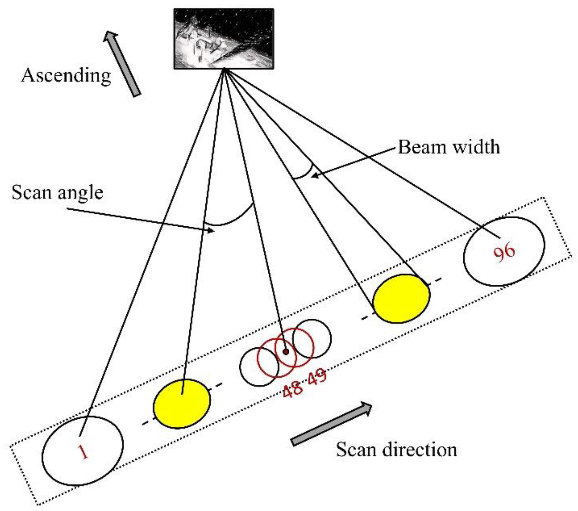
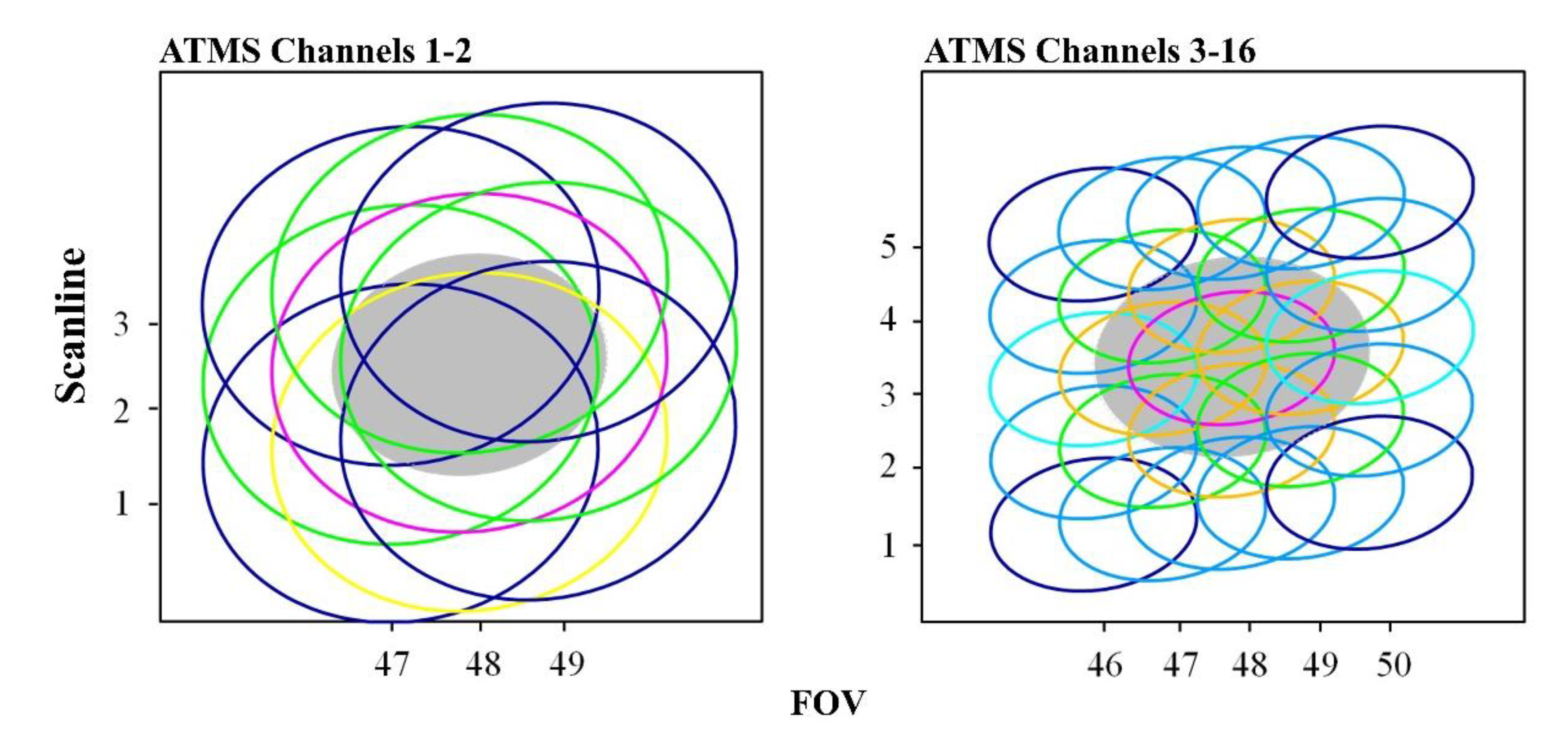
2.1. ATMS Instrument

ATMS is designed with 22 channels at a frequency ranging from 23 to 183 GHz. It has three different spatial resolutions dependent on frequency. The antenna’s half-power beam width at two low-frequency channels at 23.8 GHz and 31.4 GHz is 5.2°; those at channels 3–16 are 2.2°, and the remaining channels are 1.1° [22]. The characteristics of each channel of the ATMS instrument are shown in Table 1. Note that NEDT was a specified value. Indeed, the actual noise of ATMS in-orbit performance is much lower than the specification [22,23].
Unifying the spatial resolution of different frequencies is of great significance for the combination of ATMS and other microwave instruments (such as AMSU-A/B) for meteorological and climate research [24,25]. ATMS collects 96 field of views of measurements across each scan shown in Figure 1. For channels 1 and 2, the field-of-view (FOV) size corresponds to 5.2° of antenna the beam width whereas for channels 3–16, the FOV size is about 2.2°. The FOVs are overlapping in both cross-track and along-track directions.
At each individual FOV, the ATMS antenna brightness temperature T a is a function of the brightness temperatures convolved by the antenna gain G as:
T a = T b ρ G ρ d A
where T b represents the brightness temperature observed by FOV.

2.2. Backus–Gilbert Inversion

Using the 3 × 3 or 5 × 5 FOVs in both cross-track and along-track directions, the overlapping information can be used to construct the brightness temperature of the target field as shown in the gray area in Figure 2. The resampled antenna brightness temperature can also be derived as:
T a B G ( k ) = i = N c h N c h j = N c h N c h a k + i , j T a ( k + i , j )
where N c h = 1   for   channel   1 2 2   for   channel   3 16 , i , and j usually refer to the direction along the scan line and across the scan line and a k + i , j represents the resampling coefficient. Therefore, the BGI resampled brightness temperature T a B G is estimated as a linear combination of the adjacent observed T a . In Equation (2), the two-dimensional window is transformed into a one-dimensional form. Mathematically, it is an ill-conditioned linear inversion problem, and regularization must be carefully considered in order to suppress the amplification of noise during inversion [26]. A dynamic balance is required between resolution and noise. The resampling coefficient a k + i , j can be obtained by minimizing the error function Q :
Q = i = N c h N c h j = N c h N c h a k + i , j G k + i , j F ρ 0 , ρ 2 d A cos ( γ ) + ( T r m s ) 2 ω sin ( γ )
where F ρ 0 , ρ represents the target antenna gain, that is, the antenna gain with a half-power width of 3.3°; γ is the noise suppression coefficient, which can vary from 0 to π/2. When γ is 0, the resolution enhancement effect is the most obvious, but the result will be full of noise. When γ is π/2, the noise is better suppressed, and the result is only the weighted average of adjacent windows. Δ T r m s is the channel noise of the instrument; the parameter ω is the scaling factor, which is to make the variables have the same order of magnitude. According to previous research, ω is taken as 0.001 [27]. The details of solving for the coefficients a k + i , j can be found in [7]. The calculation of the resampling coefficient a k + i , j requires the antenna gain G . In this study, the antenna gain G is simulated by a Gaussian increasing function and projected onto the geodetic coordinate system. Additionally, the size of the antenna main beam is considered to be 2.5 times the half-power width.
In this paper, the ellipse-shaped FOV points are mapped to the equal latitude and longitude projection, and the FOV points are gridded with a resolution of 0.1°. The coefficient training time grows significantly as the resolution increases. The optimal coefficients at each scan point location can be reused.

2.3. AAPP Resampling Algorithm

The method of fast Fourier transform can be used to adjust the beam width of the antenna. In the frequency domain the convolution between brightness temperature and antenna gain can be simplified to multiplication, so Equation (1) can be expressed as:
T a ζ = T b ζ G ^ ζ
where ζ is the frequency and represents the fast Fourier transformation. It is known that the Fourier transformation of a Gaussian distribution is still a Gaussian distribution. So, in the frequency domain, it is easy to simulate the antenna gain using the Gaussian function. Since T b ζ is constant for T a ζ with any antenna width, we have:
T t a r g e t ζ = T s o u r c e ζ G ^ t a r g e t ζ G ^ s o u r c e ζ
The ratio of target to source antenna gain in the frequency domain on the right side of Equation (5) is an adjustment factor M . Finally, the brightness temperature after beam adjustment can be obtained through the inverse Fourier transform. In order to check and balance the noise, the adjustment factor needs to be regularized, which is expressed as:
M = G ^ t a r g e t ζ G ^ s o u r c e ζ exp ( ( ln G ^ t a r g e t ζ ) 2 ln 2 ( ln c ) 2 ) 0 < c < 1 G ^ t a r g e t ζ G ^ s o u r c e ζ c = 0
where c is the noise balance parameter and ranges from 0 to 1. For the case of enhanced resolution, the optimal value of c is 0.4. If c is further reduced, the noise is sharply amplified. To achieve the effect of noise suppression, M should be less than M , which is satisfied when the parameter c moves between 0 and 1. When resolution smoothing is implemented to reduce noise, there is no need to suppress noise, and parameter c is set to 0.
The AAPP algorithm can be implemented in the following four steps: the first step is to pad the image to a power of 2 in each dimension; the second step is to perform the fast Fourier transform and extract the real part of the complex number; the third step is to calculate the adjustment coefficient according to the Equation (6) and multiply it by the brightness temperature in the frequency domain; finally, an inverse fast Fourier transform is performed to obtain the antenna brightness temperature after the beam adjustment. Additionally, the AAPP algorithm only takes the orbital files of brightness temperature as inputs and performs image resolution processing through an adjustment in the frequency domain. The physical implication of this algorithm is not as comprehensive as the BGI algorithm.

2.4. Modified AAPP Resampling Algorithm

According to previous research and experiments, it is found that the AAPP resampling algorithm has some issues with the enhancement of image resolution, especially in the region with a large temperature gradient. The noise cannot be well suppressed if the parameters c are reduced. In the frequency domain, the brightness temperature after the fast Fourier transform is multiplied by the adjustment term to achieve the effect of resolution reconstruction. The adjustment factor directly affects the performance of the algorithm. Based on the AAPP resampling algorithm, a new form of adjustment factor is proposed and defined as:
M = ( G ^ t a r g e t ζ ) α G ^ s o u r c e ζ exp ( ( 1 G ^ t a r g e t ζ ) ln ( c k ) )
where c is still the noise balance parameter; different from M in Equation (6), this paper puts the polynomial part outside the exponent, and does not fix it in the form of a binary function but uses the parameter α to control the order of the polynomial; the parameter k is the scaling factor that makes c vary over a small range. The values of α and k in this paper are 4 and 100, respectively.
Figure 3a,b compare the beam adjustment effects from two algorithms. The blue and green curves are the Gaussian distribution function (GDF) after the Fourier transform, corresponding to two antenna beam widths of 3.3° and 5.2° respectively. Equations (6) and (7) are used for computing GDFs. It can be seen that in the frequency domain, a larger antenna beam width results in a narrower GDF as shown in the green curve. The black solid and dash lines show two GDFs corresponding to two adjustment factors to the 5.2° antenna beam width. In the original AAPP resampling algorithm, a larger c has a stronger capability to suppress the noise. When the parameter c approaches 0, the adjusted beam gradually approaches the 3.3° beam, as shown by the black solid line in Figure 3a. In the modified AAPP resampling algorithm, we no longer pursue the coincidence of the beams, because the noise caused by the pursuit of the coincidence of the beams cannot be suppressed during the image enhancement. As shown in Figure 3b, the smaller c has a stronger ability for noise suppression. When c is 0.1, the difference between the adjusted beam and the 5.2° beam is very small; as c increases, the adjusted beam becomes wider and wider and gradually approaches the 3.3° beam or is better than 3.3°.

2.5. Algorithm Evaluation and Verification

In this study, BGI, AAPP, and modified AAPP resampling algorithms are compared by applying them to ATMS detailed as follows:
(1)
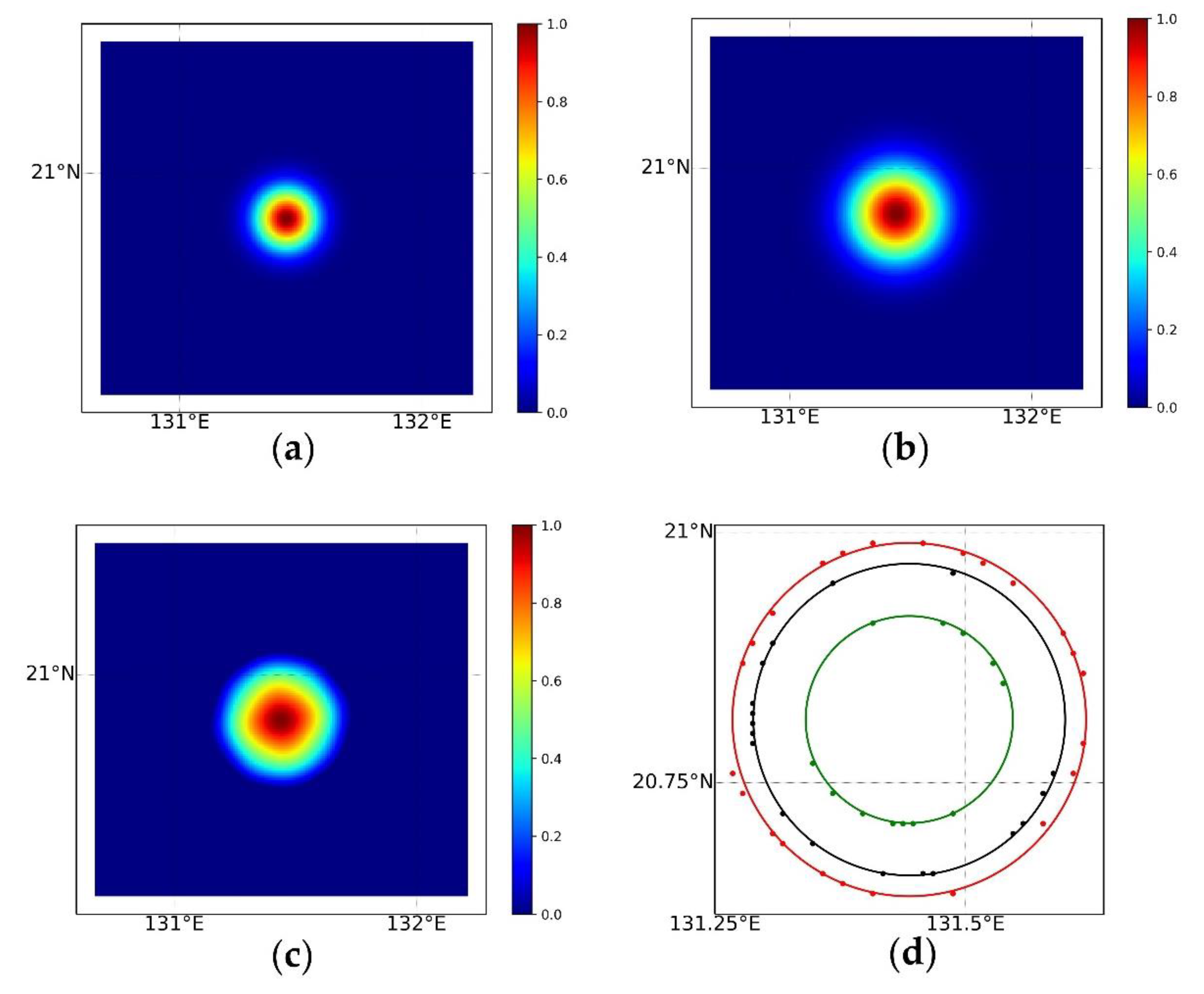
For the BGI method, the antenna gain function (AGF) projected to the geographic coordinate system can be used for qualitative evaluations. However, this verification method does not work for frequency domain algorithms.
(2)
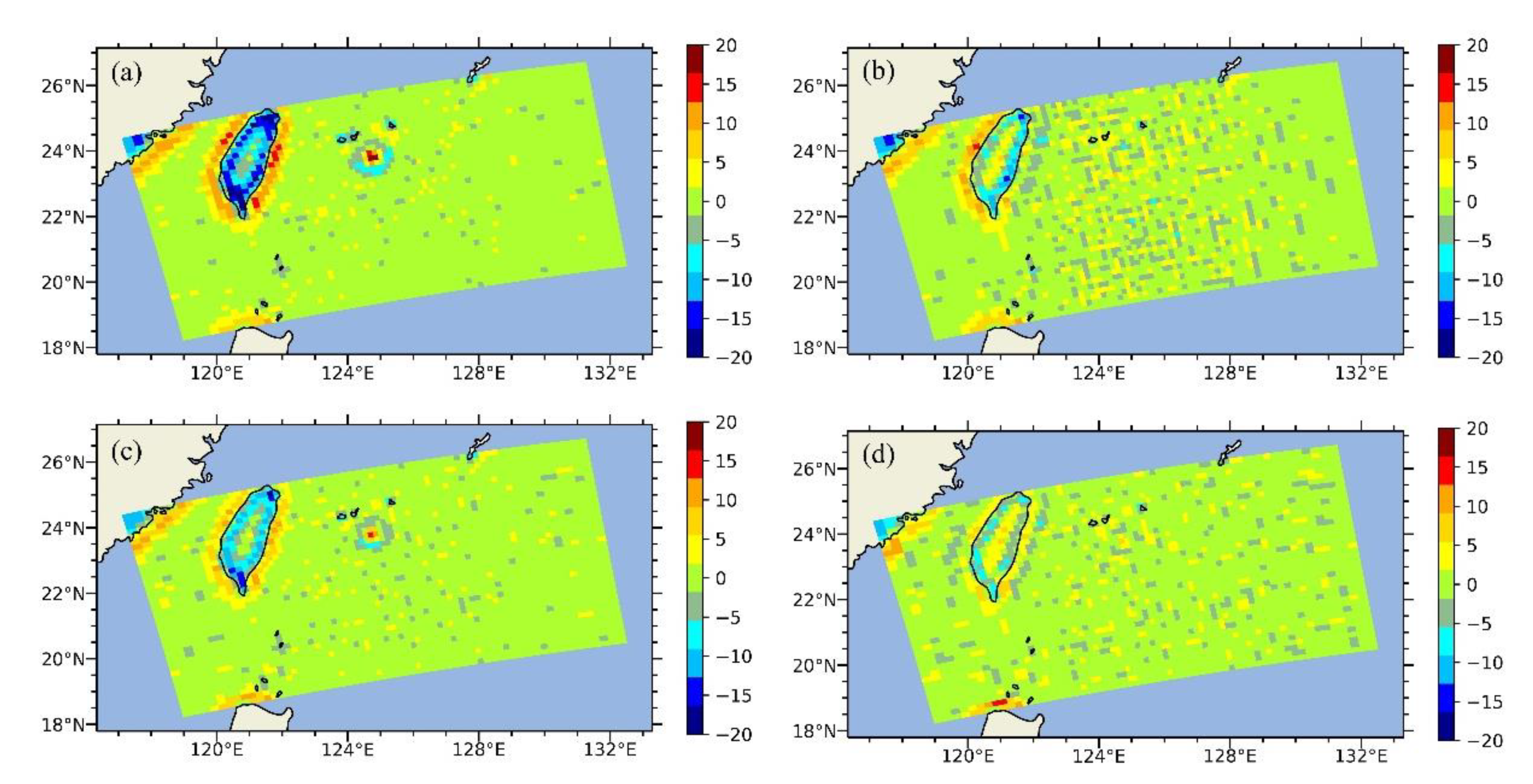
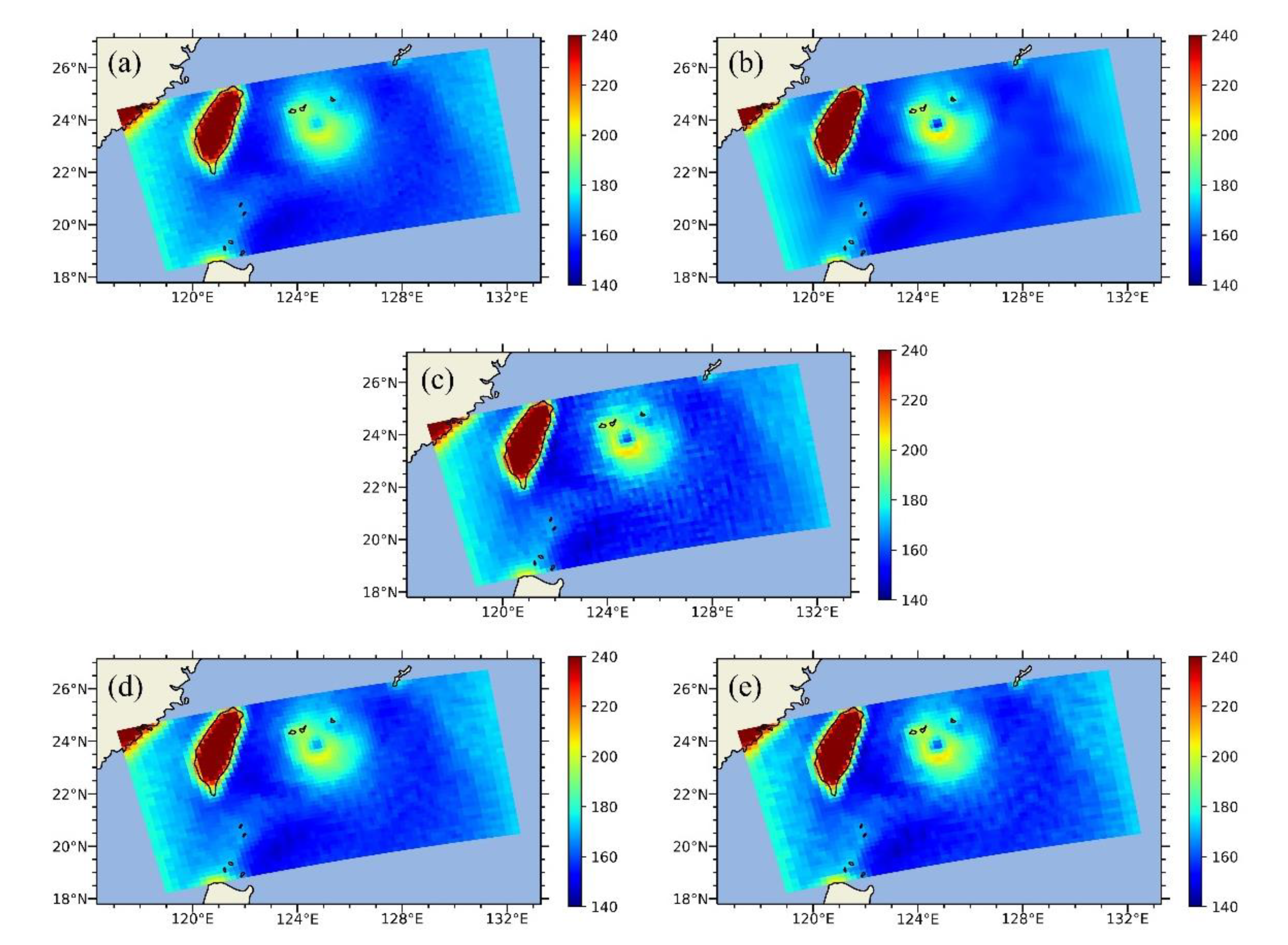
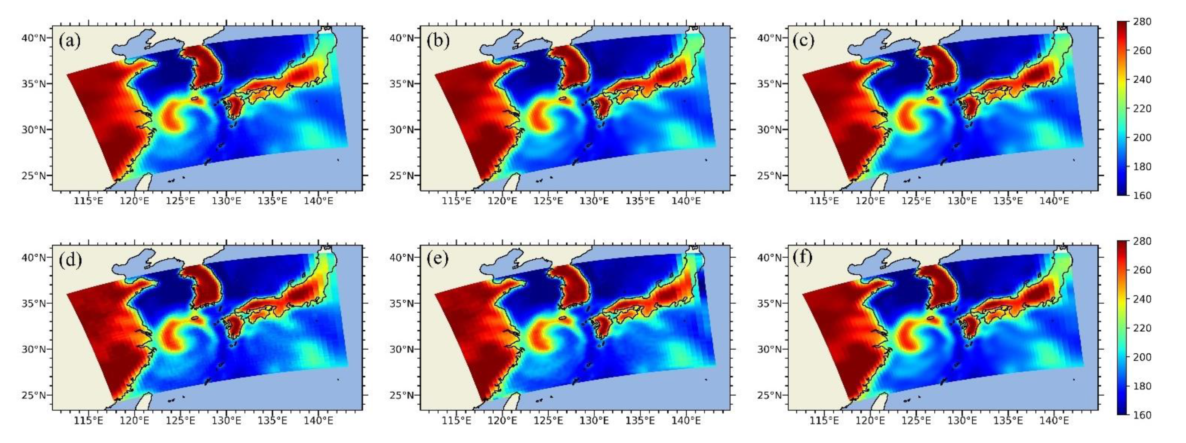
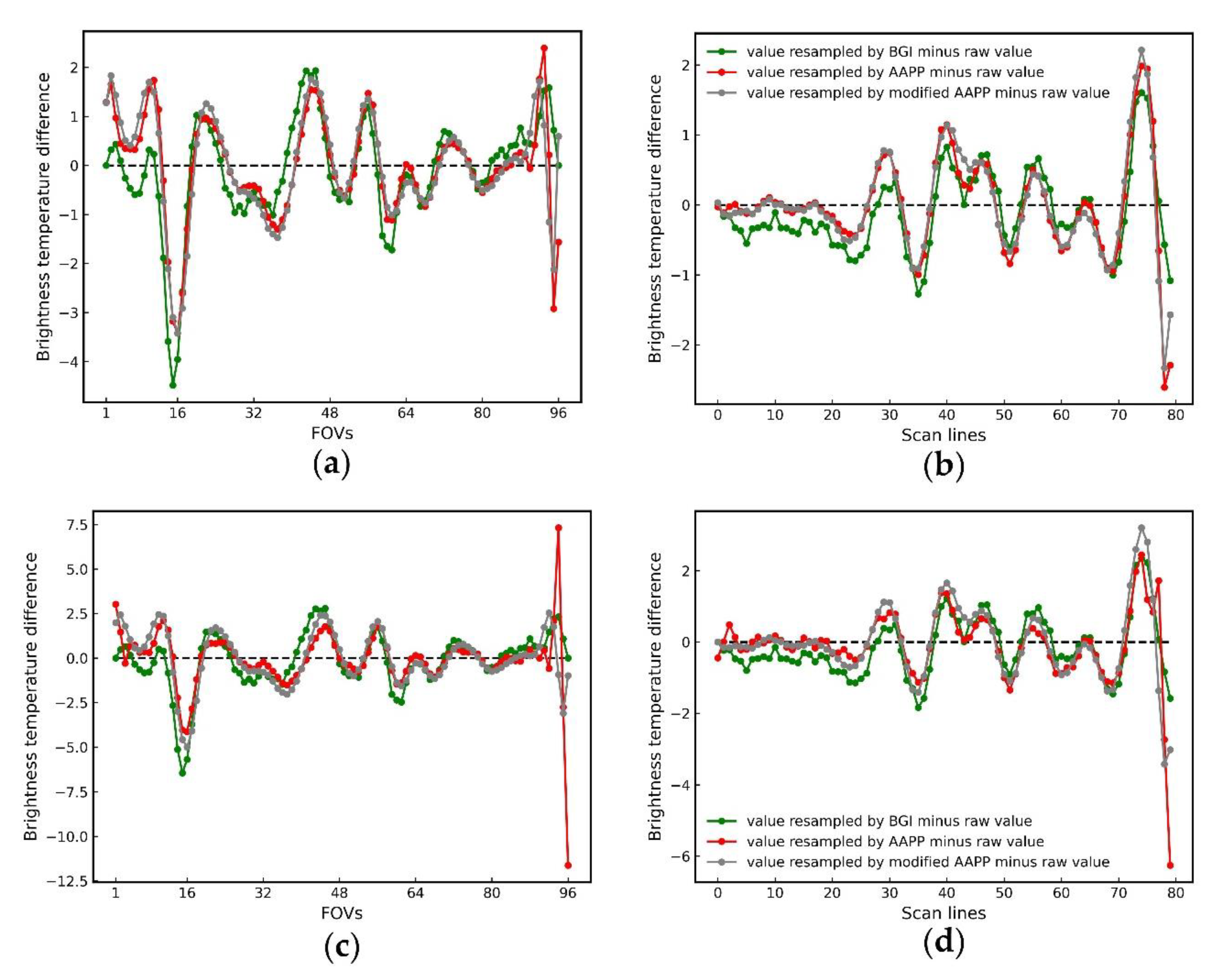
Quantitative evaluations are performed using the radiative transfer model simulation results. First, the atmospheric and surface parameters of typhoon Lekima on 8 August 2019, are generated using the weather research and forecasting (WRF) model with a resolution of 3 km. Then, these outputs are used as inputs to the fast radiation transfer model ARMS (advanced radiative transfer modeling system) [28] to simulate the ATMS brightness temperatures at 22 channels. The brightness temperature fields are used to construct the actual scene brightness temperature T b . It is worth noting that when using ARMS to simulate the brightness temperature, the limb effect of ATMS is taken into account. Finally, the AGFs of different antenna sizes are convolved with T b to obtain the ATMS antenna temperature T a according to Equation (1). The antenna temperature with an AGF beam width of 3.3° simulated by the model can be used as the true value, so that the qualitative and quantitative evaluations of the BGI, AAPP, and modified AAPP resampling algorithms can be carried out.
Using mean absolute error (MAE), root mean square error (RMSE), and BIAS for quantitative evaluation, the calculation formula is as follows:
MAE = 1 m i = 1 M T t r u e T r e s a m p l e d
RMSE = 1 m i = 1 M T t r u e T r e s a m p l e d 2
BIAS = 1 m i = 1 M T t r u e T r e s a m p l e d
where T t r u e is the true value simulated by the ARMS, and T r e s a m p l e d is the brightness temperatures from resampling algorithms.
(3)
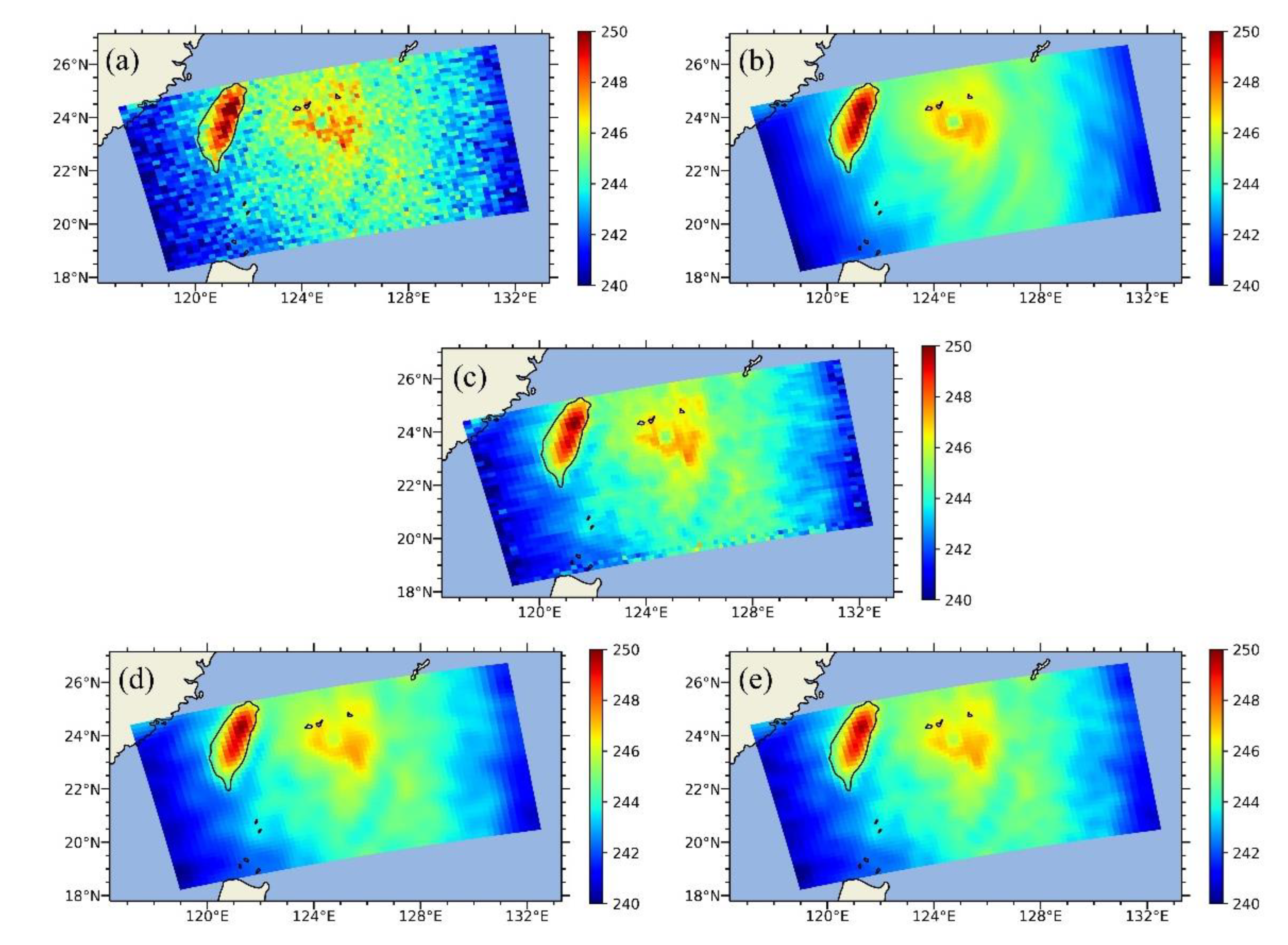
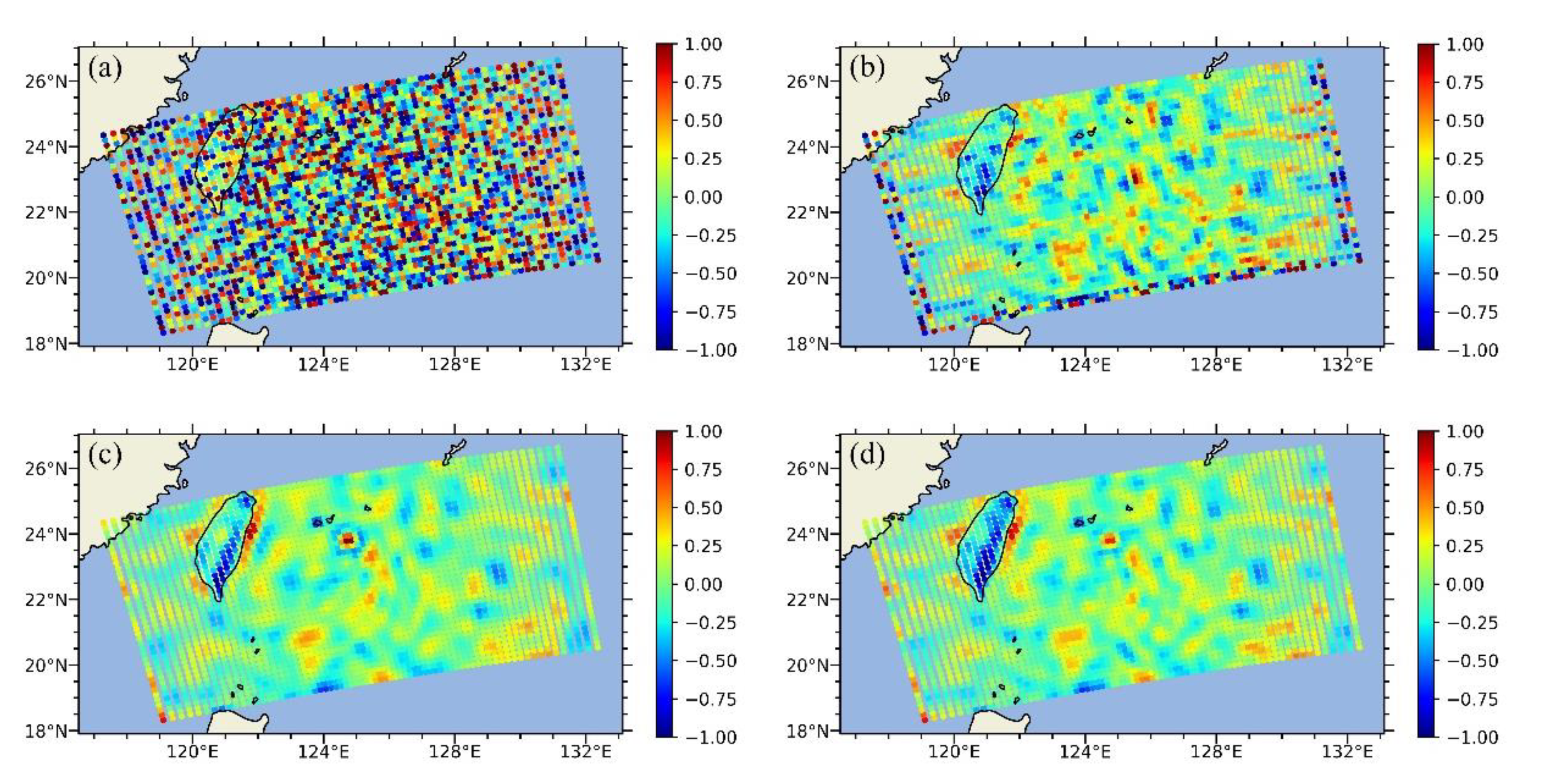
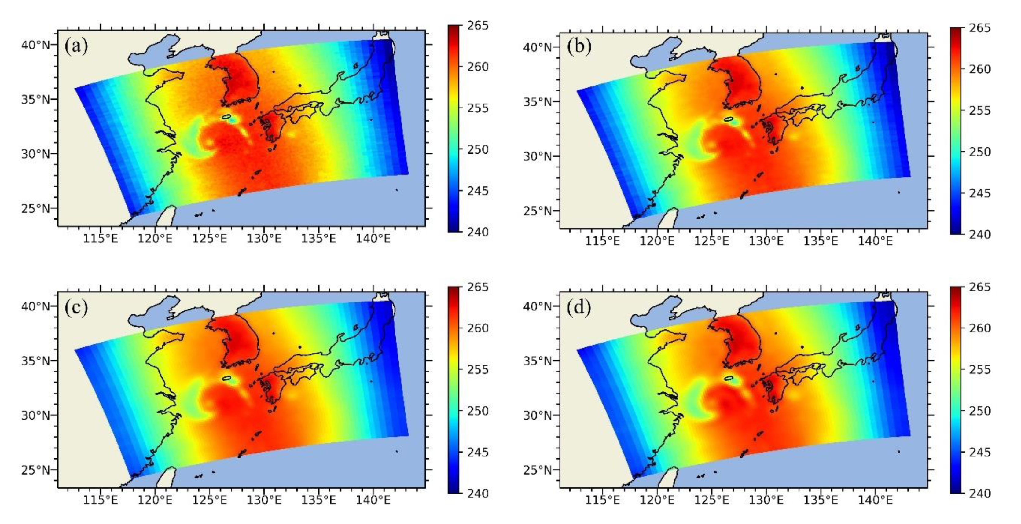
Observed ATMS data from NOAA-20 satellites are also used for qualitative assessments.

3. Results

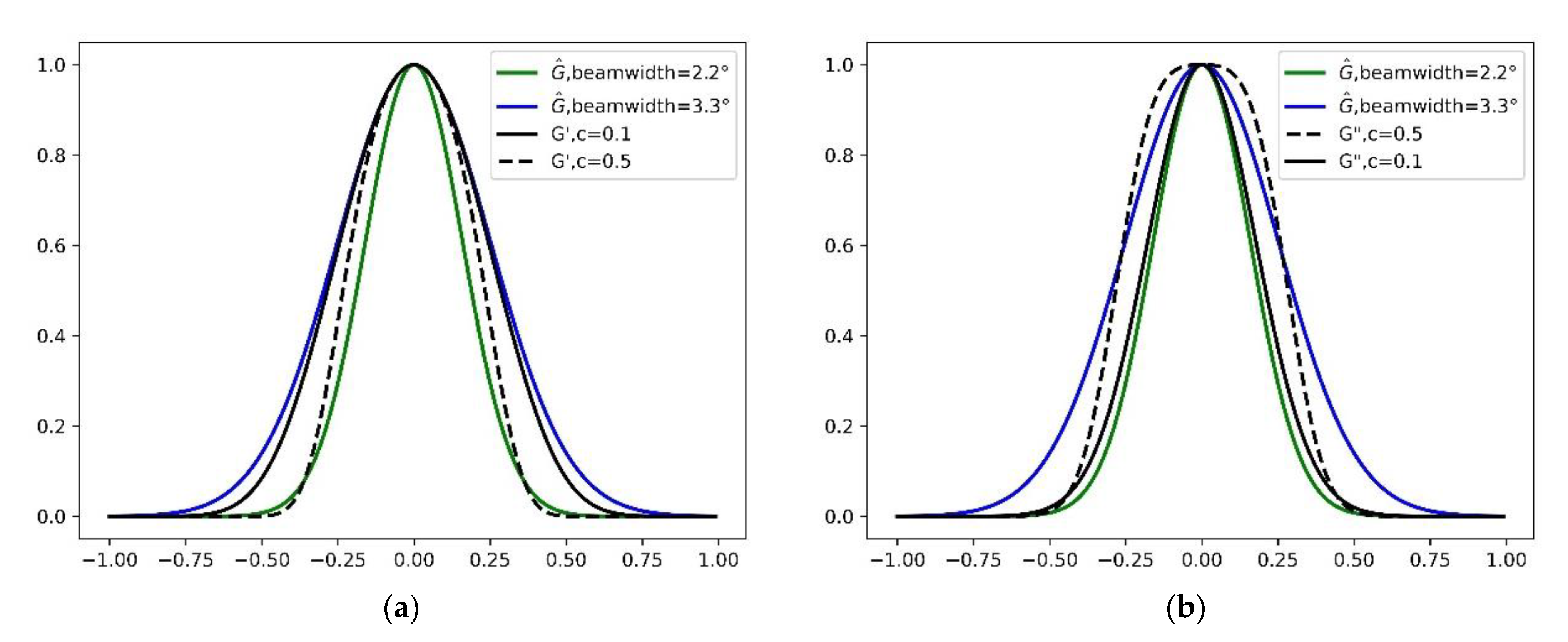
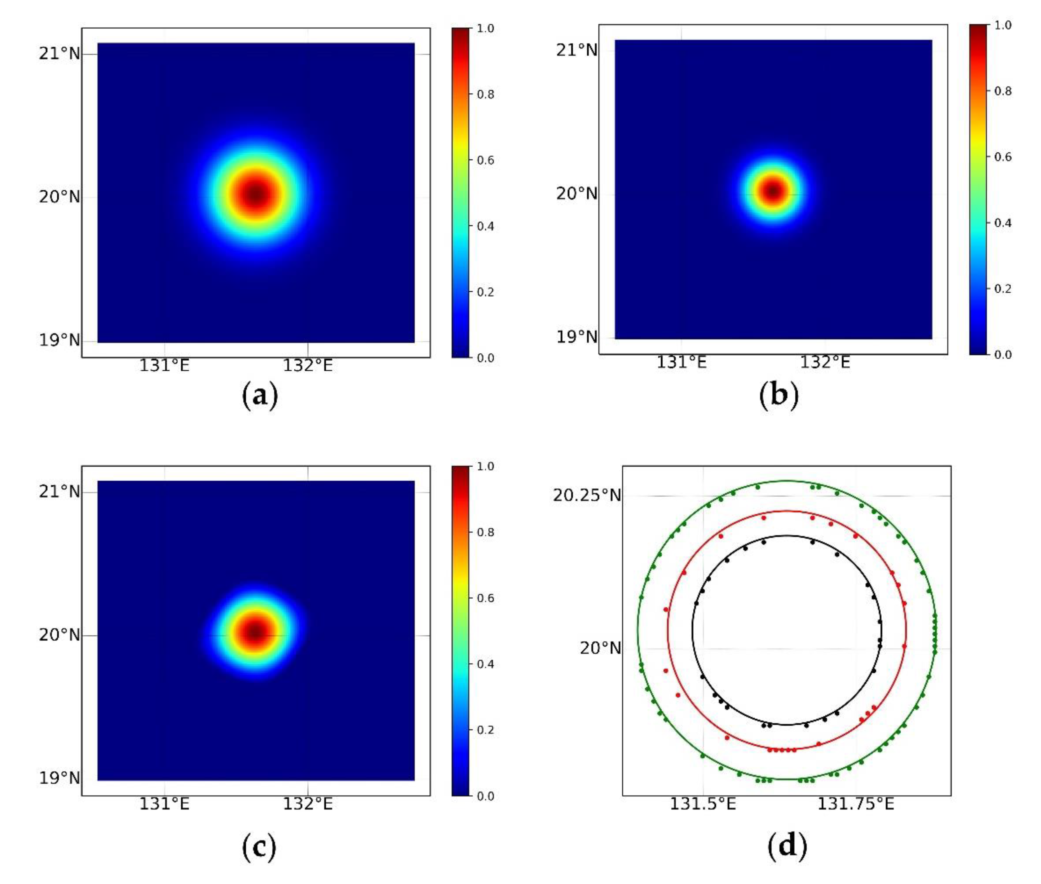
3.1. Antenna Gain Function Reconstructed by BGI

When calculating the resampling coefficients by the BGI method, the overlapping information between the AGFs is a key element. So, it may be useful to apply resampling coefficients to the AGF to characterize the effect of resolution reconstruction. Figure 4 and Figure 5 show the results of resolution enhancement and resolution reduction, respectively. Figure 4a,b are the normalized AGFs of 5.2° and 3.3° at the sub-satellite point position in the geographic coordinate system, respectively; Figure 4c is the result of nine overlapping AGFs as shown in Figure 2 with a half-power beam width of 5.2° resampled by BGI. It can be seen that the AGF after BGI resolution enhancement is smaller and narrower than the original AGF, which means that its high-weight value is closer to the center. In order to more intuitively display the effect of resolution reconstruction, the half-power points (points with a value of 0.5) in the AGF are extracted, and these points are fitted in the form of circles, as shown in Figure 4d. The green and black curves and points are the half-power circle and half-power points of 5.2° and 3.3°, respectively, while the red curve and points are the half-power circle and half-power points after resolution enhancement. From Figure 4d, it can clearly be seen that the beam width is narrower.
Figure 5a is an AGF with a half-power width of 2.2°, Figure 5b is an AGF with a half-power width of 3.3°, Figure 5c is the target AGF resampled by BGI using adjacent 5 × 5 AGFs with a half-power width of 2.2°. All AGFs are normalized. Figure 5d are the half-power curve and half-power points obtained by AGFs. The amplification of the source AGF and the increase of the half-power width can be seen. As can be seen from Figure 4 and Figure 5, the BGI method can realize the reconstruction of spatial resolution, the resolution reduction appears to be easier than resolution enhancement, and the reconstructed half-power fitted curve is closer to the target value.
By reconstructing the AGF, we can better understand how the BGI algorithm works. However, it cannot fully represent the relationship between resolution and noise. Specifically, it cannot reveal the noise amplification effect caused by resolution enhancement and the smoothing effect caused by resolution reduction. In practical applications, there is a convolution process between the AGF and the background brightness temperature, which may affect the selection of parameters.

3.2. Experiments and Comparisons Using Simulated Brightness Temperatures

The ATMS antenna brightness temperatures are simulated by WRF-ARMS and used to evaluate the three resampling algorithms. In order to make the simulated values closer to the real observations, random noise is added to the simulated values, and the standard deviation of the noise is set to the NEDT of each channel specified in ATMS requirements. Note that this study does not add noise distribution to true values which is the simulated value with an AGF of 3.3°.
The simulated ATMS channel 2 antenna temperature and the resampling results of the three algorithms are shown in Figure 6. Figure 6a is the antenna brightness temperature of ATMS channel 2 with Gaussian noise. The half-power width and NEDT of channel 2 are 5.2° and 0.8 K, respectively; Figure 6b is the simulated noise-free antenna brightness temperature true value. Figure 6c–e are the results of the resolution enhancement of the 5.2° antenna brightness temperatures using BGI, AAPP, and modified AAPP resampling algorithms, respectively. It can be seen that the three algorithms all have the effects of enhancing the spatial resolution to a certain extent, and all have the side effect of amplifying the noise. By observing the internal structure of the typhoon, it can be found that the enhancement effect of the BGI and the modified AAPP resampling algorithm is more obvious and closer to the true value, while the effect of the original AAPP algorithm is relatively weak. However, correspondingly, the image after BGI enhancement shows more obvious noise distribution. It should be noted that the noise trade-off parameters of the three algorithms have been optimized to minimize the RMSE between the resampled brightness temperatures and the true values.
To more clearly reveal the difference between the resampling results and truth, Figure 7 shows the difference in brightness temperature and the spatial distribution of the difference. Figure 7a is the difference between the brightness temperature without image enhancement and the true value. Figure 7b–d are the difference between the brightness temperature after image enhancement and the true value, using BGI, AAPP, and modified AAPP respectively. The difference in antenna brightness temperatures with different half-power widths is very obvious, especially in the regions of weather systems such as typhoons and near coastal boundaries, see Figure 7a. Compared to Figure 7b, the active weather signals are not enhanced well from AAPP whereas the coastline and typhoon are better illustrated by BGI in Figure 7c. The enhancement effect of the BGI and modified AAPP is more consistent, but the noise level of the modified AAPP is significantly lower as shown in Figure 7d. The noises from BGI are manifested as a stripping pattern whereas those from modified AAPP appear spotty. Therefore, the modified AAPP algorithm improves the spatial structure resolution and suppresses the noise. It is the best solution for microwave sounder resampling applications.
Figure 8 shows the effect of algorithm resolution smoothing using the ATMS antenna brightness temperature at channel 6. The random noise of 0.7 K is added to simulate the antenna brightness temperature with an AGF of 2.2°, as shown in Figure 8a. Three resolution smoothing algorithms are used to obtain a noise-free antenna brightness temperature with an AGF of 3.3° as shown in Figure 8b. In resolution smoothing, the noise is obviously suppressed from three algorithms, especially using AAPP and modified AAPP. It is apparent that the BGI has a poor result in the image edge since it cannot form a 5 × 5 or 3 × 3 window. As mentioned above, the resolution reduction is easier to achieve than resolution enhancement, because it does not require the use of penalty terms to suppress noise, and the resolution reduction itself plays a role in denoising. The original AAPP excels at reduced resolution, and the modified AAPP maintains its advantages.
Figure 9 shows the distribution of differences between antenna brightness temperatures. Since ATMS channel 6 measures the microwave radiation from the upper atmosphere, antenna brightness temperatures are not sensitive to the sea-land boundary and active typhoon signals. The difference in Figure 9a shows the Gaussian noise added to the simulations. All three algorithms result in lower noise, the results of AAPP and modified AAPP are very similar but are better than those from the BGI method.
Taking the antenna brightness temperature with an AGF of 3.3° as the ground truth value, the three quality indicators of BIAS, MAE, and RMSE are calculated and are shown in Table 2. Due to the added noise to ATMS channel 2, the RMSE between antenna brightness temperatures with different AGFs can reach 3.5 K. After the resolution reconstruction algorithm is applied, the RMSE decreases to a certain extent. The commonly used BGI and AAPP algorithm can reduce the RMSE to about 2.5 K, and the modified AAPP algorithm proposed in this paper can further reduce the RMSE to about 2 K. Similarly, the MAE error with the true value is also improved. However, for BIAS, there is no obvious rule, because BIAS is originally a positive value, but becomes negative after the resolution is enhanced. For ATMS channel 6, the modified AAPP does not have much improvement compared with AAPP. Two filtering algorithms can reduce RMSE error by 70%, while BGI can only reduce it by about 60%. Other channels show the same result.

3.3. Experiments and Comparisons Using ATMS Observations

If the experiment is only carried out on the simulated data, there are uncertainties caused by the radiative transfer model and the simulation method of the antenna brightness temperature. In this section, the actual ATMS antenna brightness temperatures are used to evaluate the effect of the resampling algorithms. ATMS TDR data at 0425 UTC on 16 September 2021, are obtained from NOAA class archival.
Figure 10a–c show the resolution enhancement results from BGI, AAPP, and modified AAPP with a low RMSE for strong noise suppression whereas Figure 10d,e,g show a high RMSE or a noise suppression. However, the noise trade-off parameters of the three algorithms have their own characteristics, and it is necessary to establish a common standard for the three algorithms. For the sake of fairness, the RMSE value between the brightness temperature before and after the resolution enhancement is used as an indicator of the strength of noise suppression. Low RMSE represents strong noise suppression, and high RMSE represents weak noise suppression. For strong noise reduction, the RMSE is set to 3.5 K, and the value of the noise trade-off parameter c of the original AAPP is about 0.4. Brightness temperatures resampled by BGI (Figure 10a) appear noisy, which is in line with the above analysis. For low noise suppression, the RMSE before and after resampling is set to 5 K. At this time, the noise trade-off parameter c in the original AAPP is about 0.2. The results of BGI (Figure 10d) and AAPP (Figure 10e) appear noisy, as we expected, and the results of AAPP have obvious outliers at the edges of the image; in contrast, the results of modified AAPP (Figure 10f) not only have lower noise but also have no anomalies at the edges. It is concluded that the modified AAPP has a good noise suppression effect, and greatly improves the original resampling algorithm.
The average brightness temperature difference at each FOV and each scan line is calculated for both low RMSE and high RMSE as shown in Figure 11. In Figure 11a,b, the overall trends of the three curves are the same, and the results of AAPP are generally consistent with the results of the modified AAPP. The results of BGI are different from the filtering algorithm, but the difference can basically be kept within 1 K. On the left side of Figure 11b, the green curve oscillates, indicating that the noise amplification effect of the BGI algorithm is more obvious. In the case of high RMSE, the average brightness temperature difference varies over a larger range. It can be seen in Figure 11c,d that the red curve (results of AAPP) has a sharp increase or decrease at the tail of the curve, while the gray curve (results of modified AAPP) has no such phenomenon. At the same time, on the left side of Figure 11d, the oscillation phenomenon of BGI results is more obvious, and the AAPP results also have an oscillation phenomenon, indicating that the noise of BGI and AAPP is not well suppressed. In summary, the modified AAPP proposed in this paper not only overcomes the abnormal phenomenon of the AAPP algorithm at the edge of the image but also has a better noise suppression effect than AAPP and BGI.
Figure 12 shows the raw observations and resolution smoothing results for ATMS TDR channel 6. Figure 12a is the original observation of ATMS channel 6, and Figure 12a–c are the results of reducing the resolution using three algorithms. As can be seen from the figure, all three algorithms can achieve the effect of noise reduction, and the effect is equivalent, the difference between the three algorithms is not obvious. This is because the noise suppression function is not needed when the image resolution is smoothed.

4. Discussion

This study investigated the quality of the Backus–Gilbert inversion (BGI), AAPP resampling algorithms, and modified AAPP algorithms for ATMS resolution enhancement or reduction. The Gaussian distribution function is assumed to represent the antenna gain function (AGF). The effect of the real antenna gain on the algorithm needs to be further studied and discussed in our future studies.
It should be pointed out that the conclusions drawn in this paper are largely based on the simulated data from WRF. More studies are needed for actual observations.
In addition, when resampling the actual observation data, there is no real ATMS antenna temperature with a half-power width of 3.3°, which makes it impossible for us to quantitatively evaluate the performance of the algorithm on the actual observation data. AMSU has a spatial resolution of 3.3° and has a similar frequency design to ATMS. However, Since ATMS are carried onboard Suomi-NPP or the NOAA-20 satellites and AMSU are on other NOAA and METOP satellites, it is inconvenient to collocate the data from two different platforms. Therefore, it is worth thinking about how to quantitatively evaluate the resolution reconstruction algorithm on the actual observation data set with a target beam width of 3.3°.
In this paper, random noise with Gaussian distribution is added to different channels. For near-surface channels such as channel 1 and channel 2 which have a very large brightness temperature difference between land and ocean, the NEDT noise level of 1 K may have a very limited impact on the image. However, for those channels with small changes in brightness temperature, NEDT of 1 K can significantly reduce the image quality. Thus, when the modified AAPP is applied to ATMS observations the quality of resampled data at a particular channel is very dependent on the actual ATMS NEDT.

5. Conclusions

A spatial resolution reconstruction is a key step in microwave remote sensing data processing, which can effectively improve the data quality and application value. In numerical weather prediction models, most of the data assimilation system is well set for the observations from AMSU-A brightness temperature. Thus, BGI and AAPP have been used to unify the spatial resolution of ATMS and AMSU-A. The BGI algorithm has been widely studied and used, but the research on the AAPP algorithm is very limited to the NPW community. This study proposes a modified AAPP resampling algorithm to achieve the unification of the spatial resolution of ATMS and is expected to be applied to more microwave instruments in the future. The difference between the modified AAPP and AAPP algorithm is that the adjustment function of the half-power width of the antenna is different. A polynomial form outside the exponential rather than a binary function form inside the exponential is used to adjust the antenna gain shape in the frequency domain. In this study, the fast-radiative transfer model ARMS and mesoscale model WRF are used to simulate the antenna brightness temperatures at 2.2°, 3.3°, and 5.2°. Compared with BGI and AAPP, modified AAPP shows smaller errors and lower noise. The modified AAPP overcomes the problem of poor accuracy of AAPP in the areas with a sharp gradient in brightness temperatures such as the boundary area of land and sea and active weather systems. Compared with the BGI algorithm, the resampling accuracy does not change with scan position.
The performance of the three resampling algorithms is also evaluated on the actual observation data. The results show that when the half-power width needs to be enhanced to 3.3° or less, modified AAPP can better suppress noise and the result of modified AAPP does not have obvious numerical anomalies at the beginning and end of the scan lines which are typical of the original AAPP. In addition, the three algorithms are equally effective in smoothing the high-resolution antenna brightness temperature, and all of them can effectively reduce the noise levels.

Author Contributions

Conceptualization, Y.X. and F.W.; software, Y.X. and F.W.; validation, Y.X.; formal analysis, Y.X. and F.W.; investigation, Y.X.; resources, Y.X.; data curation, Y.X.; writing—original draft preparation, Y.X.; writing—review and editing, F.W.; visualization, Y.X.; supervision, F.W.; project administration, F.W.; funding acquisition, F.W. All authors have read and agreed to the published version of the manuscript.

Funding

This research was funded by the National Key Research and Development Program of China (2021YFB3900400) and the National Natural Science Foundation of China (U2142212).

Data Availability Statement

The ATMS TDR data can be obtained from the website of NOAA Comprehensive Large Array-data Stewardship System (CLASS) (https://www.avl.class.noaa.gov/saa/products/welcome/, accessed on 15 January 2022).

Acknowledgments

I would like to thank Hu Hao for the WRF output data and related guidance, and the ARMS team for their excellent ARMS software.

Conflicts of Interest

The authors declare no conflict of interest.

References

  1. Eyre, J.R.; Kelly, G.A.; McNally, A.P.; Andersson, E.; Persson, A. Assimilation of TOVS radiance information through one-dimensional variational analysis. Q. J. R. Meteorol. Soc. 1993, 119, 1427. [Google Scholar] [CrossRef]
  2. Yang, H.; Weng, F.; Lv, L.; Lu, N.; Liu, G.; Bai, M.; Qian, Q.; He, J.; Xu, H. The FengYun-3 microwave radiation imager on-orbit verification. IEEE Trans. Geosci. Remote Sens. 2011, 49, 4552–4560. [Google Scholar] [CrossRef]
  3. Newman, K.M.; Schwartz, C.S.; Liu, Z.; Shao, H.; Huang, X.-Y. Evaluating forecast impact of assimilating microwave humidity sounder (MHS) radiances with a regional ensemble Kalman filter data assimilation system. Weather Forecast. 2015, 30, 964–983. [Google Scholar] [CrossRef]
  4. Mangla, R.; Indu, J.; Chambon, P.; Mahfouf, J.-F. First steps towards an all-sky assimilation framework for tropical cyclone event over Bay of Bengal region: Evaluation and assessment of GMI radiances. Atmos. Res. 2021, 257, 105564. [Google Scholar] [CrossRef]
  5. Farrar, M.R.; Smith, E.A. Spatial resolution enhancement of terrestrial features using deconvolved SSM/I microwave brightness temperatures. IEEE Trans. Geosci. Remote Sens. 1992, 30, 349–355. [Google Scholar] [CrossRef]
  6. Zhou, J.; Yang, H. Comparison of the resampling algorithms for the advanced technology microwave sounder (ATMS). Remote Sens. 2020, 12, 672. [Google Scholar] [CrossRef] [Green Version]
  7. Stogryn, A. Estimates of brightness temperatures from scanning radiometer data. IEEE Trans. Antennas Propag. 1978, 26, 720–726. [Google Scholar] [CrossRef]
  8. Poe, G.A. Optimum interpolation of imaging microwave radiometer data. IEEE Trans. Geosci. Remote Sens. 1990, 28, 800–810. [Google Scholar] [CrossRef] [Green Version]
  9. Chakraborty, P.; Misra, A.; Misra, T.; Rana, S.S. Brightness temperature reconstruction using BGI. IEEE Trans. Geosci. Remote Sens. 2008, 46, 1768–1773. [Google Scholar] [CrossRef]
  10. Maeda, T. Spatial resolution enhancement algorithm based on the Backus–Gilbert method and its application to GCOM-W AMSR2 data. IEEE Trans. Geosci. Remote Sens. 2020, 58, 2809–2816. [Google Scholar] [CrossRef]
  11. Gu, H.; England, A.W. AMSR-E data resampling with near-circular synthesized footprint shape and noise/resolution tradeoff study. IEEE Trans. Geosci. Remote Sens. 2007, 45, 3193–3203. [Google Scholar] [CrossRef]
  12. Long, D.G.; Daum, D.L. Spatial resolution enhancement of SSM/I data. IEEE Trans. Geosci. Remote Sens. 1998, 36, 407–417. [Google Scholar] [CrossRef] [Green Version]
  13. Long, D.G.; Hardin, P.J.; Whiting, P.T. Resolution enhancement of spaceborne scatterometer data. IEEE Trans. Geosci. Remote Sens. 1993, 31, 700–715. [Google Scholar] [CrossRef] [Green Version]
  14. Long, D.G.; Brodzik, M.J. Optimum image formation for spaceborne microwave radiometer products. IEEE Trans. Geosci. Remote Sens. 2016, 54, 2763–2779. [Google Scholar] [CrossRef] [PubMed] [Green Version]
  15. Long, D.G.; Brodzik, M.J.; Hardman, M.A. Enhanced-resolution SMAP brightness temperature image products. IEEE Trans. Geosci. Remote Sens. 2019, 57, 4151–4163. [Google Scholar] [CrossRef]
  16. Sethmann, R.; Burns, B.A.; Heygster, G.C. Spatial resolution improvement of SSM/I data with image restoration techniques. IEEE Trans. Geosci. Remote Sens. 1994, 32, 1144–1151. [Google Scholar] [CrossRef]
  17. Dawei, L.; Kai, L.; Changchun, L.; Jungang, M. Resolution enhancement of passive microwave images from geostationary Earth orbit via a projective sphere coordinate system. J. Appl. Remote Sens. 2014, 8, 1–11. [Google Scholar] [CrossRef] [Green Version]
  18. Hu, W.; Li, Y.; Zhang, W.; Chen, S.; Lv, X.; Ligthart, L. Spatial resolution enhancement of satellite microwave radiometer data with deep residual convolutional neural network. Remote Sens. 2019, 11, 771. [Google Scholar] [CrossRef] [Green Version]
  19. Li, Y.; Hu, W.; Chen, S.; Zhang, W.; Guo, R.; He, J.; Ligthart, L. Spatial resolution matching of microwave radiometer data with convolutional neural network. Remote Sens. 2019, 11, 2432. [Google Scholar] [CrossRef] [Green Version]
  20. Yang, H.; Zou, X. Optimal ATMS resampling algorithm for climate research. IEEE Trans. Geosci. Remote Sens. 2014, 52, 7290–7296. [Google Scholar] [CrossRef]
  21. Zhou, J.; Yang, H. Noise suppression in ATMS spatial resolution enhancement using adaptive window method. In Proceedings of the 2021 IEEE International Geoscience and Remote Sensing Symposium IGARSS, Brussels, Belgium, 11–16 July 2021; pp. 7693–7695. [Google Scholar] [CrossRef]
  22. Weng, F.; Zou, X.; Wang, X.; Yang, S.; Goldberg, M.D. Introduction to Suomi national polar-orbiting partnership advanced technology microwave sounder for numerical weather prediction and tropical cyclone applications. J. Geophys. Res. Atmos. 2012, 117, D19112. [Google Scholar] [CrossRef]
  23. Kim, E.; Lyu, C.-H.; Anderson, K.; Leslie, R.V.; Blackwell, W.J. S-NPP ATMS instrument prelaunch and onorbit performance evaluation. J. Geophys. Res. Atmos. 2014, 119, 5653–5670. [Google Scholar] [CrossRef] [Green Version]
  24. Zou, C.-Z.; Wang, W. Intersatellite calibration of AMSU-A observations for weather and climate applications. J. Geophys. Res. Atmos. 2011, 116, D23113. [Google Scholar] [CrossRef]
  25. Mears, C.A.; Wentz, F.J.; Thorne, P.; Bernie, D. Assessing uncertainty in estimates of atmospheric temperature changes from MSU and AMSU using a Monte-Carlo estimation technique. J. Geophys. Res. Atmos. 2011, 116, D08112. [Google Scholar] [CrossRef]
  26. Piles, M.; Camps, A.; Vall-llossera, M.; Talone, M. Spatial-resolution enhancement of SMOS data: A deconvolution-based approach. IEEE Trans. Geosci. Remote Sens. 2009, 47, 2182–2192. [Google Scholar] [CrossRef]
  27. Robinson, W.D.; Kummerow, C.; Olson, W.S. A technique for enhancing and matching the resolution of microwave measurements from the SSM/I instrument. IEEE Trans. Geosci. Remote Sens. 1992, 30, 419–429. [Google Scholar] [CrossRef]
  28. Weng, F.; Yu, X.; Duan, Y.; Yang, J.; Wang, J. The advanced radiative transfer modeling system (ARMS)—A new generation of satellite observation operator developed for numerical weather prediction and remote sensing applications. Adv. Atmos. Sci. 2020, 37, 131–136. [Google Scholar] [CrossRef] [Green Version]
Figure 1. Schematic diagram of ATMS scan geometry. For each scan, there are a total of 96 overlapping field-of-view positions which can be used for resampling.
Remotesensing 14 02781 g001
Figure 2. Schematic diagram of resampling ATMS antenna brightness temperature using BGI (the colored hollow ellipse represents the original observation FOV, and the gray solid ellipse represents the FOV at the target resolution).
Remotesensing 14 02781 g002
Figure 3. Adjusted antenna beams in the frequency domain (a) using the original AAPP resampling algorithm and (b) using a modified AAPP resampling algorithm.
Remotesensing 14 02781 g003
Figure 4. AGFs and half-power curves of sub-satellite point; (a) AGF of 5.2°; (b) AGF of 3.3°; (c) AGF resampled by BGI; (d) half-power points and half-power curves obtained from an AGF of 5.2° (green), an AGF of 3.3° (black), and an AGF resampled by BGI (red). Note that AGF is dimensionless.
Remotesensing 14 02781 g004
Figure 5. AGFs and half-power curves of sub-satellite point; (a) AGF of 2.2°; (b) AGF of 3.3°; (c) AGF resampled by BGI; (d) half-power points and half-power curves obtained from an AGF of 2.2° (green), an AGF of 3.3° (black), and an AGF resampled by BGI (red). Note that AGF is dimensionless.
Remotesensing 14 02781 g005
Figure 6. (a) Simulated brightness temperature at channel 2 with 5.2 AGF; (b) simulated brightness temperature with 3.3 AGF (true without noise); (c) brightness temperature resampled from (a) by BGI; (d) brightness temperature resampled from (a) by AAPP; (e) brightness temperature resampled from (a) by modified AAPP. The unit of brightness temperature is K.
Remotesensing 14 02781 g006
Figure 7. Brightness temperature differences between (a) 5.2° simulations and truth value (Figure 6a,b); (b) brightness temperature differences between results resampled by BGI and truth value (Figure 6b,c); (c) brightness temperature differences between results resampled by AAPP and truth value (Figure 6b,d); (d) brightness temperature differences between results resampled by modified AAPP and truth value (Figure 6b,e). The unit of brightness temperature differences is K.
Remotesensing 14 02781 g007
Figure 8. (a) Simulated brightness temperature at channel 6 with 2.2 AGF; (b) simulated brightness temperature with 3.3 AGF (true without noise); (c) brightness temperature resampled from (a) by BGI; (d) brightness temperature resampled from (a) by AAPP; (e) brightness temperature resampled from (a) by modified AAPP. The unit of brightness temperature is K.
Remotesensing 14 02781 g008
Figure 9. Brightness temperature differences between (a) 2.2° simulations and truth value (Figure 8a,b); (b) brightness temperature differences between results resampled by BGI and truth value (Figure 8b,c); (c) brightness temperature differences between results resampled by AAPP and truth value (Figure 8b,d); (d) brightness temperature differences between results resampled by modified AAPP and truth (Figure 8b,e). The unit of brightness temperature differences is K.
Remotesensing 14 02781 g009
Figure 10. Comparisons of effects of RMSE magnitude on ATMS channel 2 resampling from three algorithms (ac) resampled by BGI, AAPP, and modified AAPP, respectively with a low RMSE; (df) resampled by BGI, AAPP, and modified AAPP, respectively with a high RMSE. The unit of brightness temperature is K.
Remotesensing 14 02781 g010
Figure 11. Average brightness temperature differences (a) at each FOV with low RMSE, (b) at each scan line with low RMSE, (c) at each FOV point with high RMSE, and (d) at each scan line with high RMSE. The unit of brightness temperature differences is K.
Remotesensing 14 02781 g011
Figure 12. ATMS channel 6 brightness temperature (a) without resampling, (b) resampled by BGI, (c) resampled by AAPP, and (d) resampled by modified AAPP. The unit of brightness temperature is K.
Remotesensing 14 02781 g012
Table 1. ATMS instrument characteristics.
ChannelCenter Frequency (GHz)NEDT(K)Beam Width (degree)
123.80.75.2
231.40.85.2
350.30.92.2
451.760.72.2
552.80.72.2
653.596 ± 0.1150.72.2
754.40.72.2
854.940.72.2
955.50.72.2
1057.2903440.72.2
1157.290344 ± 0.2170.752.2
1257.290344 ± 0.3222 ± 0.0481.22.2
1357.290344 ± 0.3222 ± 0.0221.22.2
1457.290344 ± 0.3222 ± 0.0101.52.2
1557.290344 ± 0.3222 ± 0.00452.42.2
1688.23.52.2
17165.50.51.1
18183.31 ± 70.61.1
19183.31 ± 4.50.81.1
20183.31 ± 30.81.1
21183.31 ± 1.80.81.1
22183.31 ± 10.91.1
Table 2. BIAS, MAE, and RMAE errors between the resampled antenna brightness temperature and the true value of channels 1–16.
ChannelAlgorithmBIAS (K)MAE (K)RMSE (K)
1None0.09471.84363.7254
BGI−0.13531.65222.5355
AAPP−0.05561.54432.7039
Modified AAPP−0.02151.33542.0239
2None0.07091.81153.5291
BGI−0.13611.72882.5616
AAPP−0.04111.49882.6123
Modified AAPP−0.00861.3772.0413
3None−0.01971.09471.6852
BGI−0.00010.49580.8902
AAPP0.00060.41870.6336
Modified AAPP−0.00180.42730.6411
4None−0.01890.75851.0934
BGI−0.00860.33770.5562
AAPP0.0030.29980.4421
Modified AAPP0.00670.29940.4419
5None−0.00940.61620.7925
BGI−0.00640.26770.3753
AAPP0.00770.23630.3217
Modified AAPP0.00760.23070.3162
6None0.01280.56370.7052
BGI0.00880.24150.3364
AAPP−0.01520.16210.2074
Modified AAPP−0.01460.15910.2048
7None−0.00410.57270.7153
BGI−0.00740.24740.3397
AAPP0.00540.13380.2111
Modified AAPP0.00630.16040.2323
8None0.01830.56200.7044
BGI0.01630.24190.3340
AAPP−0.01580.11700.2074
Modified AAPP−0.01380.11230.2050
9None0.00140.56030.7001
BGI0.00040.24520.3334
AAPP0.00190.15990.2264
Modified AAPP0.00210.15290.2178
10None0.00370.55430.6972
BGI0.00310.23960.3309
AAPP−0.00130.15780.2308
Modified AAPP0.00230.17010.2422
11None0.01840.59950.7843
BGI0.01630.25390.3502
AAPP−0.01680.16460.2422
Modified AAPP−0.01890.17010.2451
12None−0.00380.96841.2103
BGI−0.00280.42410.5748
AAPP0.00270.27460.3892
Modified AAPP0.00290.27580.3899
13None0.00800.96971.2165
BGI0.01100.41250.5681
AAPP−0.01460.26580.3933
Modified AAPP−0.01660.27010.3988
14None0.01701.20921.5156
BGI0.01940.53940.7388
AAPP−0.02400.35810.5211
Modified AAPP−0.02450.36020.5297
15None0.02661.91252.4030
BGI0.02300.83941.1569
AAPP−0.03010.55370.8132
Modified AAPP−0.02950.55010.8089
16None−0.07683.12314.0295
BGI−0.03771.36401.9480
AAPP0.04881.20001.6611
Modified AAPP0.04641.18921.6429
Publisher’s Note: MDPI stays neutral with regard to jurisdictional claims in published maps and institutional affiliations.

