Seeded Classification of Satellite Image Time Series with Lower-Bounded Dynamic Time Warping

Abstract

Satellite Image Time Series (SITS) record the continuous temporal behavior of land cover types and thus provide a new perspective for finer-grained land cover classification compared with the usual spectral and spatial information contained in a static image. In addition, SITS data is becoming more accessible in recent years due to newly launched satellites and accumulated historical data. However, the lack of labeled training samples limits the exploration of SITS data, especially with sophisticated methods. Even with a straightforward classifier, such as k-nearest neighbor, the accuracy and efficiency of the SITS similarity measure is also a pending problem. In this paper, we propose SKNN-LB-DTW, a seeded SITS classification method based on lower-bounded Dynamic Time Warping (DTW). The word “seeded” indicates that only a few labeled samples are required, and this is not only because of the lack of labeled samples but also because of our aim to explore the rich information contained in SITS, rather than letting training samples dominate the classification results. We use a combination of cascading lower bounds and early abandoning of DTW as an accurate yet efficient similarity measure for large scale tasks. The experimental results on two real SITS datasets demonstrate the utility of the proposed SKNN-LB-DTW, which could become an effective solution for SITS classification when the amount of unlabeled SITS data far exceeds the labeled data.

1. Introduction

With continuously-accumulating satellite images and fast-evolving analytical methodologies, studies focusing on Satellite Image Time Series (SITS) [1,2,3,4,5] began to emerge in large numbers over the last ten years. The lack of SITS data is no longer a major barrier for research and applications due to the launch of more satellites and the open access policy of historical data. Data from new satellites, such as Landsat 9 [6] and GaoFen 6 [7], are already available, and data from previous satellites, including but not limited to Landsat 5/7/8, GaoFen 1/2/4, MODIS Terra/Aqua and Sentinel 1/2, have accumulated for decades [8,9,10].

Compared with single-temporal or multi-temporal images, SITS fully records the continuous temporal behavior of land cover types, and the temporal behavior is critical for the fine-grained distinguishability of land cover types in many circumstances [11,12,13]. Different land cover types may behave similarly in one or several discrete time phases but they do not always behave the same if we observe continuously. In this paper, we separate SITS from multi-temporal images by their continuity and frequency. SITS usually consists of a longer and more continuous series of images, while multi-temporal images consist of several temporally scattered images that are either too few or too discrete to construct a SITS. Figure 1 shows an example of SITS.

Land cover is a fundamental source of information to describe or understand the environment and its changes [14,15,16]. Thus, land cover classification has become an important task for earth sciences [17,18,19]. Given SITS data, a major goal of research is to achieve more precise land cover classification results by further exploring the temporal information contained in SITS [20]. A quick review of the literature shows that many methods regarding the classification of SITS have been proposed in recent years [1,2,21,22,23,24,25,26,27,28,29,30,31,32,33,34], and these methods can be divided into three major categories: neural-network-based methods, similarity-measure-based methods, hybrid and other methods.

Neural-network-based methods focus on designing effective network architectures to extract decisive temporal features, and the network architectures have evolved from temporal convolutional networks [1,2] and recurrent neural networks [21,22], to self-attention networks [23,24,25]. Similarity-measure-based methods evaluate the similarity between labeled and unlabeled data. Currently, Dynamic Time Warping (DTW) [26,27] and its variants [28], for example, time-weighted DTW [29,30], have become some of the most widely used similarity measures for SITS. Hybrid methods include combining different classification paradigms [31], fusing time series data from different satellites with different spatiotemporal resolutions [32] and constructing new features with machine-learning models [33,34] or phenological models [31].

Despite the variety of classification methodologies, one common point for most of them is that they propose a high requirement for the amount and quality of labeled training samples. Advanced neural networks for SITS are becoming sophisticated with many network layers and millions of parameters to be tuned by a vast number of labeled data [35,36]. Similarity-measure-based methods also demand a set of high quality labeled samples to be compared with unlabeled query samples. However, in real world applications, the insufficiency of labeled samples is the normal situation, especially for land cover classification tasks. Three typical approaches for the acquisition of labeled land cover samples are listed as follows:

• Field investigation: It is labor-and-resource-consuming to send people to the investigation spots, and the number of labeled samples we can find in this way is limited. Furthermore, the labels are difficult to update.
• Visual interpretation: This relies heavily on high-spatial-resolution imagery and expert knowledge. As a consequence, class labels are sometimes unavailable for certain areas and considerable incorrect labels could be included.
• Synthesis of existing results: It is difficult to evaluate the reliability of existing land cover classification results or handle the diversity among different results due to the sparsity of validation samples and the distinctions on classification systems, map projections, etc.

The lack of labeled samples has long been noticed by researchers and many small-sample-oriented methods, for instance, transfer learning [37,38], meta learning [39,40] and knowledge distillation [41,42], have been proposed. However, these methods are essentially based on the assumption that we have sufficient labeled data or knowledge from other domains, which is also a difficult condition in many scenarios including land cover classification. In addition to the above-mentioned difficulties, temporal data analysis requires the class labels to be updated frequently, and that is scarcely satisfiable in a moderate or larger-scale case [26]. In contrast with the insufficiency of labeled data, the vast majority of SITS data are unlabeled.

Therefore, exploring the potential of unlabeled data becomes crucial for the classification of SITS, and in this way, we can achieve an all-data-driven paradigm rather than only a labeled-data-driven paradigm. In this paper, we propose SKNN-LB-DTW, a seeded SITS classification method based on the time series similarity measure of lower-bounded DTW [43,44]. The word “seeded” indicates that we employ only a few labeled samples for each class to serve as the seeds that guide the k-nearest neighbor classifier [45], instead of requiring numerous labeled samples to train a classifier.

We choose DTW as the similarity measure for k-nearest neighbor classifier because DTW is capable of coping with time distortions. Since DTW has a quadratic computational complexity [46], multiple levels of lower bounds, such as LB_Kim and LB_Keogh [44,47,48] are employed to avoid unnecessary calculations of DTW and accelerate the whole process. The proposed method maintains a moderate influence of training samples and attempts to make the rich information contained in SITS data be the decisive factor.

To demonstrate the performance of our method, two SITS datasets of full-size Landsat 8 images from year 2013 to 2017 were constructed. Cloud and cloud shadow pixels were mended by information transfer [49,50] from other images in the same SITS to ensure that the temporal information was continuous enough to reflect the temporal evolution of land cover types. Compared with several benchmark methods that are still usable with few labeled samples, our method exhibits improved accuracy, and compared with raw DTW, our method can save approximately half of the time.

The main contributions of this work are summarized as follows:

• The proposed method only requires a few labeled samples and can achieve relatively high accuracy. This means the method has wider availability in more applications. We use limited samples not only because the lack of labeled samples is a common phenomenon but also because we tend to dig the rich information of unlabeled SITS data and keep a balance between the influence of labeled and unlabeled data.
• The proposed method employs the combination of cascading lower bounds and early abandoning of DTW to greatly accelerate the classification process while maintaining exactly the same results. This is especially significant for SITS datasets because satellite images usually contain millions of pixels, and the direct calculation of DTW will take an unacceptable amount of time.
• The proposed method introduces a seed-selection strategy from existing land cover classification products if no labeled samples is available. The strategy aims to keep only the “correctly-labeled” samples by a set of morphological and statistical approaches. The strategy is totally unsupervised, which enables the automatic classification of SITS in a large or even global scale.

The remainder of this paper is organized as follows. Section 2 systematically describes DTW, the lower bounds of DTW, the early abandoning of DTW and the entire process of seeded classification of SITS. Section 3 details the datasets, settings, statistical and visual results of the SITS classification experiments. Section 4 discusses the contributions of lower bounds and the limitations of SKNN-LB-DTW. Finally, Section 5 concludes this work.

2. Materials and Methods

2.1. Dynamic Time Warping

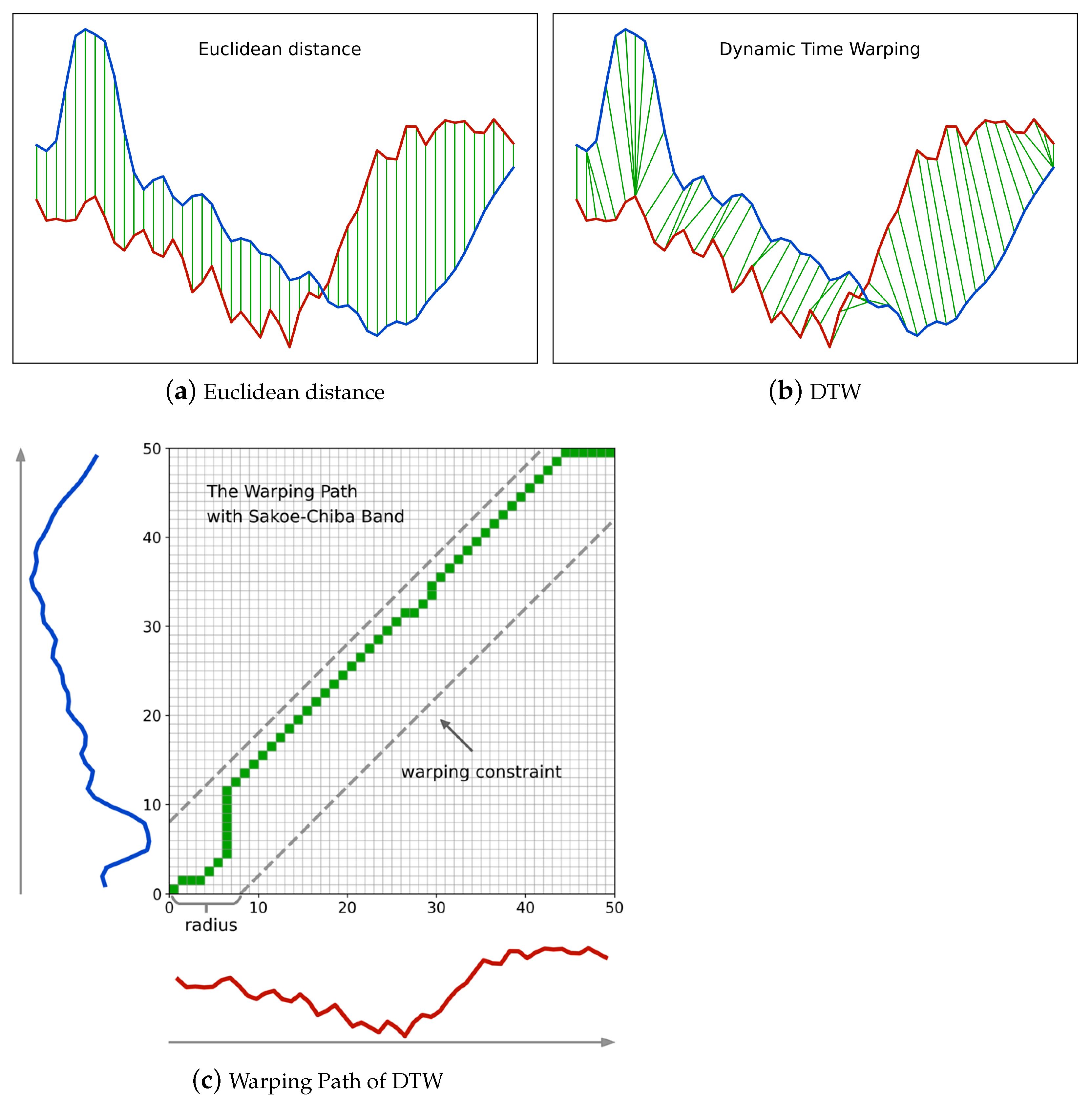
A similarity measure is a fundamental tool for k-nearest neighbor classification of SITS [51,52]. Currently, Euclidean distance and Dynamic Time Warping (DTW) [53,54] are the two most widely used similarity measure prototypes. Figure 2a,b illustrates Euclidean distance and DTW, respectively. We observe that Euclidean distance imposes a temporally linear alignment between time series, while DTW is more flexible, and non-linear alignment is allowed in a temporally local range. The flexibility of DTW enables it to cope with time distortions effectively and makes DTW a more suitable similarity measure for complex SITS data.

To give a quantitative definition of Euclidean distance and DTW, let $A=\{a_1,a_2,\cdots ,a_i,\cdots ,a_I\}$ and $B=\{b_1,b_2,\cdots ,b_j,\cdots ,b_J\}$ be two time series of length I and J. The lowercase $a_i$ and $b_j$ with subscript i and j denote the i-$th$ and j-$th$ elements of time series A and B, respectively. The cost between the i-$th$ element of A and the j-$th$ element of B is denoted by $d(i,j)$. In this setting, the Euclidean distance between A and B can be formulated as:

$$\begin{array}{cc}\hfill EUC(A,B)& =\sum _{k=1}^{I}d(k,k)\hfill \\ \hfill I& =J\hfill \end{array}$$

(1)

where $d(k,k)={(a_k-b_k)}^2$ skips the usual square-root operation to save more calculation time, and the squared version does not influence the result of the k-nearest neighbor classifier.

As for DTW, its flexibility comes from its attempt to find an optimal alignment that achieves a minimum accumulated cost between two time series. Unlike the Euclidean distance, in DTW the k-$th$ element of A is not always aligned with the k-$th$ element of B, and thus a warping path is used to record each pair of aligned elements. The warping path is usually denoted by $W=w_1,w_2,\cdots ,w_k,\cdots ,w_K$, where each time warp $w_k=(i,j)$ denotes a pair composed of $a_i$ and $b_j$. The length of the warping path is the uppercase K.

Figure 2c shows the warping path in correspondence with Figure 2b, where the x-coordinate and y-coordinate of each matrix cell in the warping path are also the indices of elements in the two time series, respectively. The final accumulated cost between the two time series, namely the DTW distance, is the sum of all pairwise costs. In this setting, DTW can be formulated as:

$$\begin{array}{cc}\hfill DTW(A,B)& =\underset{W}{min}\sum _{k=1}^{K}d\left(w_k\right)\hfill \\ \hfill w_1& =(1,1)\hfill \\ \hfill w_K& =(I,J)\hfill \\ \hfill 0\le & i^{\prime }-i\le 1\hfill \\ \hfill 0\le & j^{\prime }-j\le 1\hfill \end{array}$$

(2)

where $w_k=(i,j)$, $w_{k+1}=(i^{\prime },j^{\prime })$ and $d\left(w_k\right)=d(i,j)={(a_i-b_j)}^2$.

Equation (2) is more of a conceptional definition of DTW than a solution. DTW, as defined by Equation (2), is a typical dynamic programming problem that can be solved by a more straightforward recursive formula:

$$DTW(A_i,B_j)=d(i,j)+min\left\{\begin{array}{c}DTW(A_i,B_{j-1})\hfill \\ DTW(A_{i-1},B_j)\hfill \\ DTW(A_{i-1},B_{j-1})\hfill \end{array}\right.$$

(3)

where $DTW(A_i,B_j)$ is the partial DTW distance between sub-sequences composed of the first i elements of A and the first j elements of B. $DTW(A_I,B_J)=DTW(A,B)$ is the final DTW distance between the two entire time series.

Based on the fact that if two elements from different time series are temporally too far, their correlation tends to be weak and they should not be paired together, many constraints on DTW have been proposed to limit the warping path inside a warping window [55,56]. Among these constraints the Sakoe–Chiba band [53] as shown in Figure 2c is the most intuitive yet effective one. Given a radius r of the Sakoe–Chiba band, the temporal difference of two time series elements $|i-j|$ cannot exceed r for any time warp $w_k=(i,j)$ in a warping path. In addition, the Sakoe–Chiba constraint is a prerequisite for LB_Keogh, a lower bound of DTW that will be used in our method and will be introduced in the next subsection. Thus, we adopt the Sakoe–Chiba constraint throughout this work.

2.2. Lower Bounds of DTW

As the name implies, a lower bound of DTW is a value that is guaranteed to be smaller than DTW. If the computation speed of a lower bound is significantly faster than DTW, then the lower bound can be used to prune off unpromising candidates and thus speed up the k-nearest neighbor search of time series. For example, suppose the threshold distance for a candidate B to be the k-nearest neighbor of a time series A is $\delta$. If a lower bound distance between A and B is $LB$ and $LB>\delta$, then we can be sure that the DTW distance $DTW>LB>\delta$ since $DTW>LB$ is guaranteed, and because of $DTW>\delta$, which means the distance is too far, the candidate can be pruned off, and the calculation of DTW can be safely skipped.

In this manner, a portion of time-consuming calculations of DTW can be replaced by the faster calculations of lower bounds, and thus the entire k-nearest neighbor classification process is accelerated. The use of lower bounds still maintains exactly the same result as the raw DTW rather than generating an approximate result.

Besides the computation speed, tightness is another important property for a lower bound. Tightness indicates how close the lower bound is to the original measure. If the tightness is high, more candidates will be pruned off and vice versa. Usually there is a tradeoff between the tightness and the computation speed of a lower bound, and thus it is difficult to find the best lower bound to use. Since each single lower bound has its weakness, a classic strategy is to use different kinds of lower bounds in a cascade. For example, we can first employ a fast lower bound to reject some obvious outliers and then employ a tight lower bound to maintain a high prune rate. In our method, we use LB_Kim [48] as the fast lower bound and LB_Keogh [44,47] as the tight one for DTW.

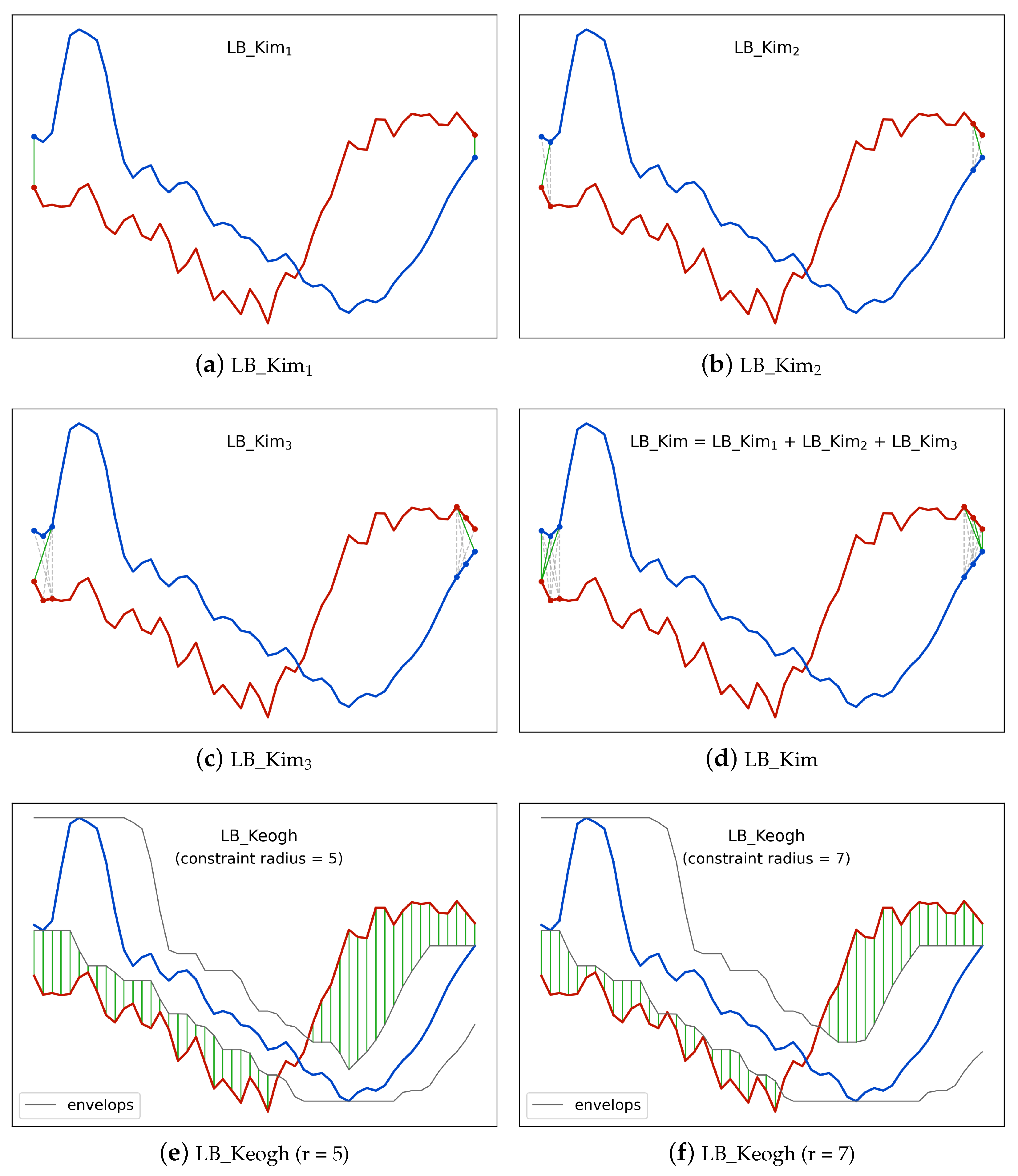
Equation (4) shows the definition of LB_Kim and it has a computational complexity of $O\left(1\right)$, which is the fastest possible situation. Figure 3 illustrates an examples of LB_Kim. The full LB_Kim is the sum of three parts. The first part LB_Kim${}_1$ as shown in Figure 3a considers the minimum possible cost among the starting elements and the ending elements of the two time series given the rule of DTW. Similarly, the second part LB_Kim${}_2$ as shown in Figure 3b further considers the minimum possible cost among the first two and the last two elements, and the third part LB_Kim${}_3$ as shown in Figure 3c considers the situation for the first three and the last three elements. Figure 3d shows the combination of the three parts.

$$\begin{array}{cc}\hfill LB\_Ki{m}_1(A,B)=& d(1,1)+d(I,J)\hfill \\ \hfill LB\_Ki{m}_2(A,B)=& min\left\{d\right(1,2),d(2,1),d(2,2\left)\right\}\hfill \\ \hfill +& min\left\{d\right(I-1,J-2),d(I-2,J-1),d(I-2,J-2\left)\right\}\hfill \\ \hfill LB\_Ki{m}_3(A,B)=& min\left\{d\right(1,3),d(2,3),d(3,3),d(3,2),d(3,1\left)\right\}\hfill \\ \hfill +& min\left\{d\right(I-1,J-3),d(I-2,J-3),d(I-3,J-3),d(I-3,J-2),d(I-3,J-1\left)\right\}\hfill \\ \hfill LB\_Ki{m}_{}(A,B)=& LB\_Ki{m}_1(A,B)+LB\_Ki{m}_2(A,B)+LB\_Ki{m}_3(A,B)\hfill \end{array}$$

(4)

where $d(i,j)={(a_i-b_j)}^2$ is the cost between the i-$th$ element of A and the j-$th$ element of B.

In contrast with LB_Kim, LB_Keogh achieves a higher tightness by comparing one time series with the upper and lower envelopes of the other time series. Equation (5) defines the envelopes of time series and Equation (6) defines LB_Keogh. The upper or lower envelope consists of a sequence of local maximum or local minimum values for a sequence of sliding windows centered at each element of a time series. The length of the sliding window is $2*r+1$ where the r is the radius of the Sakoe–Chiba band of DTW. In this setting, LB_Keogh is guaranteed to be smaller than DTW, and the proof can be found in [47]. Given a pair of envelopes, LB_Keogh sums the cost caused by elements larger than the upper envelope and elements smaller than the lower envelop. Figure 3e,f illustrates the LB_Keogh with different Sakoe–Chiba band radii.

$$\begin{array}{cc}\hfill U& =u_1,u_2,\cdots ,u_i,\cdots ,u_I\hfill \\ \hfill L& =l_1,l_2,\cdots ,l_i,\cdots ,l_I\hfill \\ \hfill u_i& =max\{a_{max(i-r,1)}:a_{min(i+r,I)}\}\hfill \\ \hfill l_i& =min\{a_{max(i-r,1)}:a_{min(i+r,I)}\}\hfill \end{array}$$

(5)

where r is the radius of the Sakoe–Chiba band of DTW, and $a_i$ is the i-$th$ element of time series A. U and L have the same length I as A and $1\le i\le I$.

$$LB\_Keogh(A,B)=\sum _{i=1}^I\left\{\begin{array}{c}{(b_i-u_i)}^{2}if{b}_i>u_i,\hfill \\ {(b_i-l_i)}^{2}if{b}_i<l_i,\hfill \\ 0otherwise\hfill \end{array}\right.$$

(6)

where $b_i$, $u_i$ and $l_i$ are the i-$th$ element of time series B, upper envelope U and lower envelope L, respectively.

For cascading lower bounds, we calculate LB_Kim first, and if LB_Kim is smaller than the current k-nearest neighbor threshold, we calculate LB_Keogh. If LB_Keogh is still smaller than the threshold, we calculate DTW. In this manner, we create two additional chances to skip the time-consuming calculation of DTW.

2.3. Early Abandoning of DTW

For a k-nearest neighbor classification problem, the similarity measure is used to decide whether a time series is close enough to be the neighbor of another time series. As soon as we know the distance between two time series is already too large to be neighbors, the calculation of distance can be abandoned to save more time. For many similarity measures we cannot know the interim results until the full calculation is completed; however, fortunately, DTW is calculated in an incremental manner, and we can obtain the interim result at each step. 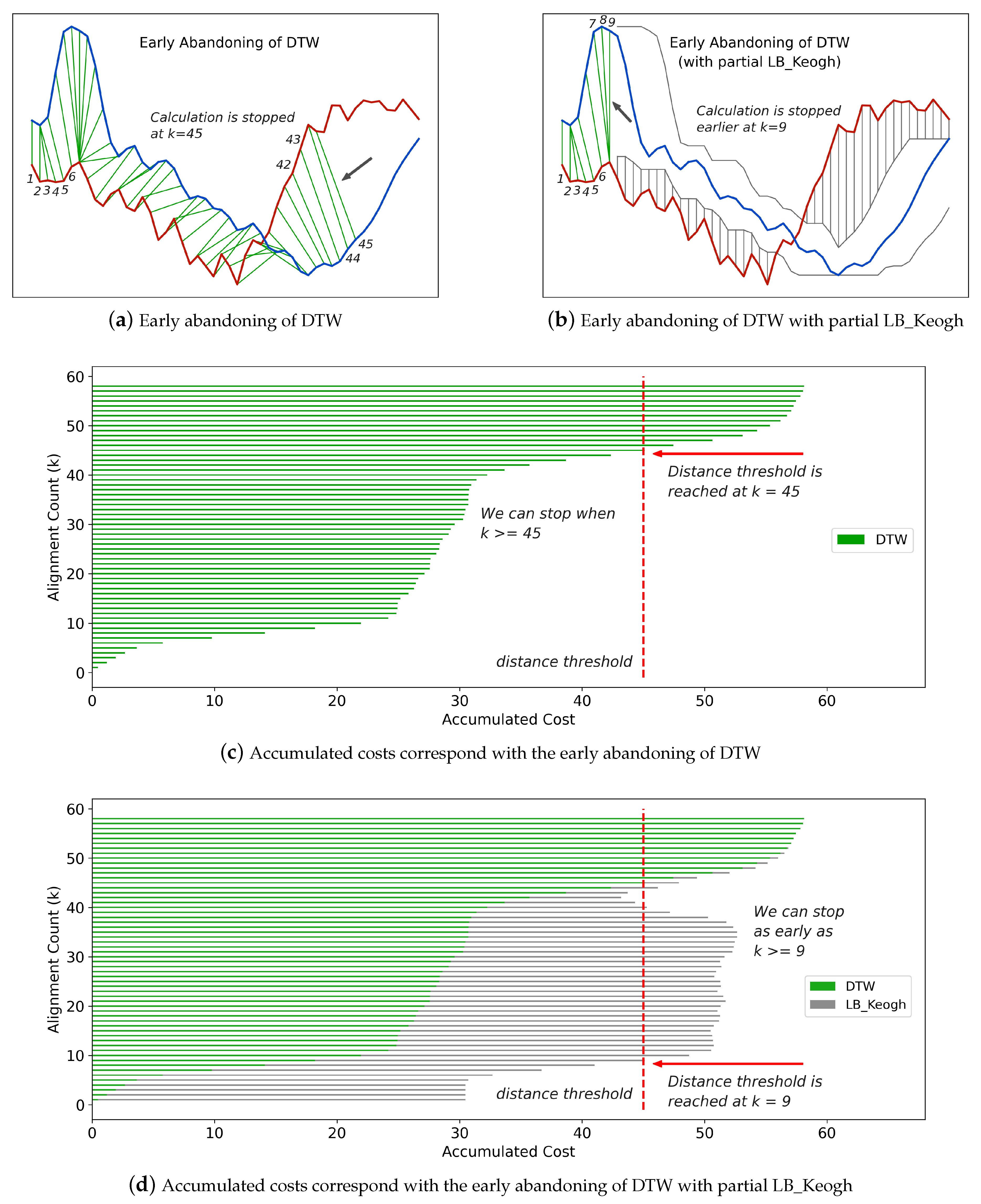Figure 4a illustrates an example of early abandoning of DTW, and Figure 4c shows the corresponding accumulated costs at each step. From Figure 4c, we observe that the distance threshold is reached at the 45th step, and correspondingly in Figure 4a, the calculation of DTW is abandoned at the 45th step.

Another trick to make the abandoning happen even earlier is to adopt partial LB_Keogh during the calculation of DTW [48]. At any step k, compared with $DTW(A_k,B_k)$, the sum of $DTW(A_k,B_k)+LB\_Keogh(A_{k+1:I},B_{k+1:I})$ is a closer lower bound to the full DTW distance $DTW(A_I,B_I)$. With the LB_Keogh contribution from $k+1$ to I, we can always predict the full DTW distance and thus conclude whether the distance will exceed the threshold in an earlier step. Figure 4b,d illustrates the use of partial LB_Keogh and its corresponding accumulated costs at each step. We observe that with partial LB_Keogh the abandoning happens at as early as the ninth step.

2.4. Seeded Classification of SITS

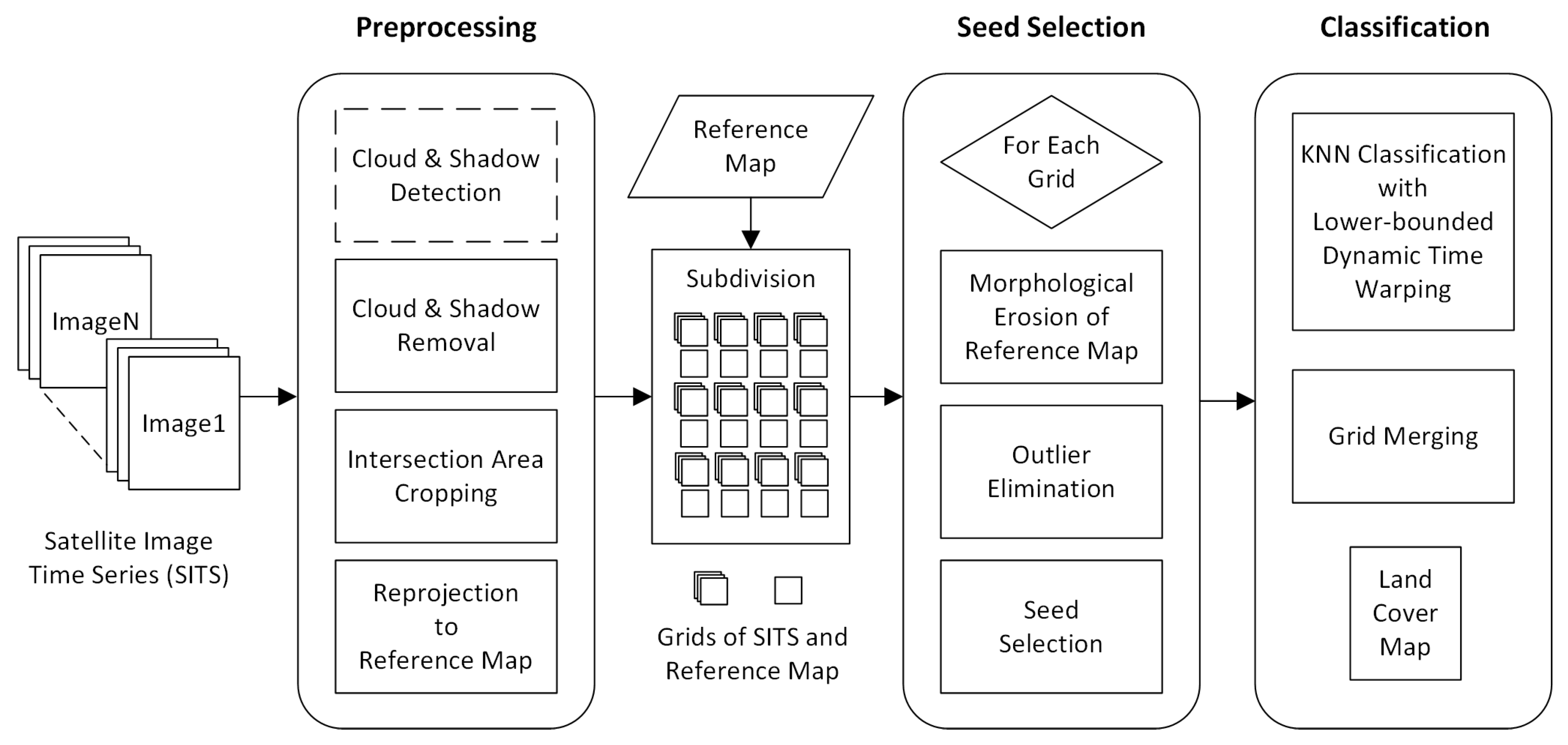
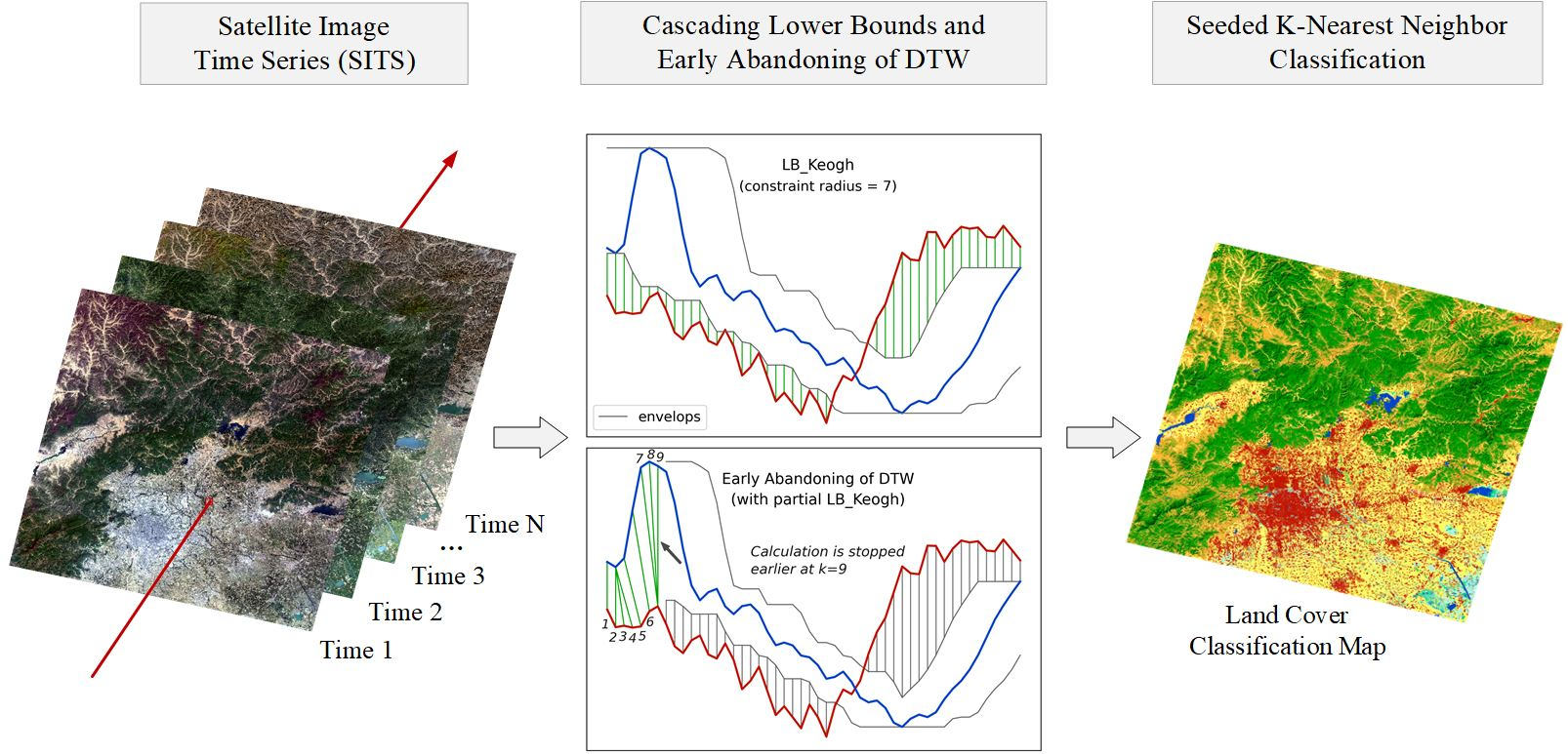
After the description of DTW based similarity measure combinations, in this subsection we present the whole process of the proposed seeded classification method for SITS. Figure 5 shows the complete flow chart with three main stages. The first stage is the preprocessing of SITS data. Optical satellite imagery usually contains massive cloud and shadow contaminated pixels. In order to ensure the continuity of temporal information, one major task is to recover cloud and shadow contaminated pixels for each image in a SITS.

If there is no cloud and shadow mask, cloud and shadow detection has to be conducted beforehand. Then, we use the information transfer method proposed in [50] to recover contaminated pixels. For each cloud or shadow contaminated image patch, the method searches for a similar image patch from the same geographical location in other images of the SITS, and then Poisson blending [57] is employed to make image patches transferred from other images fit seamlessly into the current image. For images that are too cloudy to recover, we must skip them.

For many satellites, such as Landsat 8 and GaoFen 1, images with the same tile number do not cover exactly the same spatial scope due to some linear offsets. Thus, we crop the intersection area of all images in a SITS to ensure pixels with the same coordinates in different images cover the same spatial scope and all time series have the same length. If a reference classification map with training labels is used for seed selection, we need to reproject all images to the same map projection system and spatial resolution as the reference map.

Due to the large size of satellite images, a full-size SITS with dozens of images will cost hundreds or thousands gigabytes of memory, which is difficult to satisfy by conventional computers. Therefore, images and the corresponding reference map have to be subdivided into multiple grids. In this work, the size of grids is $600\times 600$.

The second stage of the process is the selection of labeled seeds for each land cover class. We select seeds from existing land cover classification products, such as FROM-GLC30 [58] or GLC-FCS30 [59]. With the aim of exploring the rich information contained in SITS data, rather than letting the training samples dominate the classification results, we strictly limit the number of seeds for each class.

Concretely, suppose the number of seeds for a class is denoted by S, the total number of samples of that class in the reference map is N, and the number of nearest neighbors is K for the classifier. Then, we make $S=max(\sqrt[e]{N},ceil(K/2))$. The former part $\sqrt[e]{N}$ greatly condenses the number of samples, for example, $\sqrt[e]{1,000,000}\simeq 161$, and it also makes the number of seeds proportional to the ground truth in general. The latter part $ceil(K/2)$ allows tiny classes to exist by giving them the minimum number of samples required by the k-nearest neighbor classifier.

Since the numbers of seeds are limited, the quality of seeds becomes critical. We adopt two techniques, one morphological and one statistical, to select more correctly classified samples and enhance the reliability of seeds. We first morphologically erode [60] all class labels in the reference map to keep only the central pixels of each land cover patch, because the central pixels usually have a higher possibility to be correctly classified. Then, we use the statistical isolation forest [61,62] algorithm to keep only the inliers, and finally seeds are randomly selected from the inliers according to the given quantity. If the number of selected seeds for a class is less than $ceil(K/2)$, we randomly select non-repeated samples before the erosion for complements.

Given the seeds and SITS data, the third stage is the k-nearest neighbor classification. The seeds are used as the training samples and the combination of cascading lower bounds and early abandoning of DTW are used as the similarity measure. The classification is conducted by grids and results of all grids are finally merged into one land cover map.

Concretely, for each input sample to be classified, we first find the K closest training examples of it, and then it is classified by a plurality vote of the K closest neighbors. To search for the K closest training examples, we iterate through all training samples and check whether a training sample is close enough to be the top K closest ones. However, we do not calculate the DTW distance directly because of its high computational complexity. Instead, we calculate the lower bounds of DTW first to prune off unnecessary calculations of DTW.

If a lower bound is already too large to make a training sample one of the K closest neighbors, then the calculation of DTW for this training sample is unnecessary because DTW is guaranteed to be larger than its lower bounds. The threshold to decide whether a training sample belongs to the top K closest ones is the DTW distance between the current k-$th$ closest training sample and the input sample. If lower bounds are smaller than the threshold, we calculate the DTW and compare the DTW distance with the threshold. To accelerate each single calculation of DTW, the early abandoning strategy can be adopted because DTW can be calculated incrementally.

During DTW calculation, we observe the interim result at each step and as soon as the threshold is reached, we know this training sample is already too far to be the top K closest neighbors and the calculation can be abandoned safely. If a training sample is closer than the threshold, then it will replace one of the old K closest neighbors, and the threshold should be updated by the new k-$th$ closest distance. In the entire classification process, we do not abandon the classification of any sample but we abandon the unnecessary calculations during the search for the K closest neighbors. All samples will be classified as the standard k-nearest neighbor classification.

It is worth noting that the process as a whole is actually unsupervised because the seed selection is unsupervised, and the succeeding classification turns unsupervised without manually training sample preparation. This enables the automatic classification of SITS in a large or even global scale.

3. Results

3.1. Datasets and Reference Samples

To demonstrate the accuracy and efficiency of the proposed SKNN-LB-DTW method for SITS, in this section we conduct classification experiments on two SITS datasets. The two datasets each consist of 40 full-size Landsat 8 images from year 2013 to 2017 with a spatial resolution of 30 m. Figure 6 shows the temporal distributions of images in the two SITS. Each element in a time series contains seven features, namely the seven surface reflectance bands (Ultra Blue, Blue, Green, Red, NIR, SWIR1 and SWIR2) of Landsat 8 imagery. Images in each SITS were preprocessed by cloud and shadow removal, intersection area cropping and reprojection as described in Section 2.4. Thus, images in each SITS cover the same spatial scope and pixels are aligned throughout the image sequence.

The first SITS locates in path 123 and row 032 of the WRS-2 (Worldwide Reference System) tiles adopted by Landsat 8 satellite. The spatial scope covers most part of Beijing city and its north. After cropping and reprojection, the image size is $9637\times 7385$. The second SITS with path 122 and row 032 locates in the adjacent tile to the east of the first SITS. The image size is $9507\times 7376$. The GLC-FCS30 2010 land cover classification product is used as the reference map for seed selection, and thus we inherit the classification system of the GLC-FCS30 product, which considers 29 fine-grind land cover classes in total.

3.2. Experimental Settings

The proposed SKNN-LB-DTW method is compared with Euclidean distance based seeded classification (SKNN-EUC), Support Vector Machine (SVM) [63,64,65] and Decision Tree (DT) [66,67,68]. Euclidean distance is the benchmark similarity measure for time series because of its robustness and accuracy. SVM is a widely used classifier that is effective in high dimensional spaces even with only a subset of training points in the decision function. DT is able to learn multiple decision rules inferred from data features and performs well even if its assumptions are violated to some extent.

In this paper, we focus only on non-deep learning methods due to the severe lack of training samples in practice, and we choose these competing methods also because they are relatively accurate even with limited training samples. For SKNN-EUC, we use the same classification process as the proposed SKNN-LB-DTW method except for the similarity measure. For DT, we employ the classification and regression trees (CART) [69,70] algorithm.

Since SVM and DT cannot handle time series data directly, we apply SVM and DT to SITS by flattening time series into one vector. For example, a time series of length 40 and 7 features $(40,7)$ can be flattened into a vector of size $(40\times 7,1)$. All these classifiers are implemented by the scikit-learn machine learning package in Python. To ensure a fair competition, if any parameter is involved, we use the optimal one, and we use the same random number generator for different methods.

3.3. Experimental Results

Figure 7 displays one example image and the classification map generated by the proposed SKNN-LB-DTW method for each SITS datasets. We can assume the classification maps represent the land cover of year 2015 because the datasets contain images from year 2013 to 2017, and year 2015 is the central year. We select the two images in Figure 7 because they are the temporally nearest cloud-free images to year 2015, and thus they are more probable to show the ground truth. An intuitive visual impression shows that spatial details, such as boundaries and textures are well preserved. For a more detailed look, Figure 8 shows a comparison between our method and the competing methods in multiple image grids with typical land cover types.

In addition, one representative image from the SITS and the reference land cover product to choose seeds from are also illustrated for each grid. The location of these grids are marked by red squares in Figure 7. We observe that water boundaries, fragmented impervious surfaces, terrain changes, building and road shapes are more accurately captured by the seeded classification method.

For a statistical evaluation of these methods, we chose four typical grids with different landscapes from the two SITS datasets. The size of the grids is $600\times 600$ pixels, and the locations are marked by yellow squares in Figure 7. The first grid mainly consists of impervious surfaces, croplands and wetlands. The second grid mainly consists of forests, grasslands and rivers. The third grid mainly consists of croplands, forests and grasslands. The fourth grid mainly consists of herbaceous covers, impervious surfaces and grasslands.

We selected these grids because they contain more temporal-varying land covers to better demonstrate the performance of time series analysis methods. For instance, the first grid is a large artificial wetland near cities, and wetland classification is challenging due to frequent temporal changes. The croplands and inland waters largely contained in these grids involve seasonal changes, and thus they are suitable targets to evaluate the capability of SITS classification methods. Expanding cities reflect temporal changes caused by human activities and they are also included in these selected grids. In addition, the balance of the sizes of land cover classes are considered.

The performance of each method is evaluated with the three most widely used criteria: the Overall Accuracy, Weighted F1 Score and Cohen Kappa Score. The overall accuracy is a straightforward performance metric, which is defined as the fraction of correct predictions. The F1 score is the harmonic mean of precision and recall of a classifier. The Cohen Kappa score is a statistic that measures the agreement between two classification results. All of the three criteria usually range in $[0,1]$, and a higher value indicates a better result.

Figure 9 shows the classification maps generated by different methods for the first grid, together with the corresponding validation samples and a reference image from the SITS. As the temporal range of the SITS is from year 2013 to 2017, we presume the date of the results is the central year 2015. Validation samples are selected manually with the help of very high resolution Google Earth images in 2015, and the proportion of classes is also considered. From Figure 9, we observe that the rainfed cropland and herbaceous cover (yellow) are well recognized by all the four methods.

However, the boundary of impervious surfaces (brown red) is not well captured by DT. SVM misclassifies a portion of irrigated cropland (light blue) and wetlands (cyan green) into water (blue). The two seeded classification methods, SKNN-EUC and SKNN-LB-DTW, basically capture most of the land cover classes well. Compared with SKNN-EUC, SKNN-LB-DTW maintains neater boundaries and more complete shapes of some water body, wetland and irrigated cropland patches, which are difficult land cover classes to distinguish.

Table 1. Statistical comparison of the classification performance for the first grid.

Method		DT	SVM	SKNN-EUC	SKNN-LB-DTW
Overall Accuracy	Local Seeding	0.582	0.760	0.844	0.882
	Global Seeding	0.433	0.667	0.623	0.605
Weighted F1 Score	Local Seeding	0.580	0.747	0.839	0.880
	Global Seeding	0.433	0.662	0.606	0.588
Cohen Kappa Score	Local Seeding	0.498	0.708	0.810	0.854
	Global Seeding	0.316	0.596	0.545	0.523
Elapsed Time (seconds)	Local Seeding	0.453	18.469	11.172	243.641
	Global Seeding	1.306	203.256	28.154	1282.277

shows the statistical comparison of the four methods for the first grid. SKNN-LB-DTW consistently achieves the best results in terms of the three criteria with margins of $3.8\%$, $4.1\%$ and $4.4\%$ compared to the second best result for each respective criterion. The statistical evaluation in Table 1 coincides with the visual impression in Figure 9. We note that two seeding schemes, local seeding and global seeding, are also compared in Table 1. Recall that the full-size satellite images have to be subdivided into multiple grids for hardware reasons, and the succeeding classification procedure is executed by each grid.

Local seeding indicates that we select seeds from the current grid, which usually results in less but more-relevant seeds. In contrast, global seeding indicates that we select seeds from the entire image, which results in more but less-relevant seeds. Statistical results show that local seeding always leads to higher accuracies by large margins, and it demonstrates that the quality of seeds plays a more important role than the quantity of seeds in our method.

Similarly with Figure 9, Figure 10 shows the classification maps, validation samples and a reference image of the second grid. We observe that SVM fails to recognize different types of forests (green and darker green) in a large portion. Wetlands (cyan green) close to the river are misclassified as forests (dark green) by DT. Furthermore, a part of impervious surfaces (brown red) are confused with sparse vegetation (beige) by DT.

SKNN-EUC and SKNN-LB-DTW capture most of the land cover classes accurately, while they still have many differences in detailed.

Table 2. Statistical comparison of the classification performance for the second grid.

Method		DT	SVM	SKNN-EUC	SKNN-LB-DTW
Overall Accuracy	Local Seeding	0.720	0.764	0.844	0.870
	Global Seeding	0.646	0.770	0.705	0.690
Weighted F1 Score	Local Seeding	0.702	0.729	0.831	0.865
	Global Seeding	0.627	0.732	0.667	0.656
Cohen Kappa Score	Local Seeding	0.636	0.686	0.798	0.831
	Global Seeding	0.536	0.698	0.612	0.592
Elapsed Time (seconds)	Local Seeding	0.500	21.719	11.422	174.218
	Global Seeding	1.418	210.292	31.062	1124.103

shows the statistical comparison of the four methods for the second grid. SKNN-LB-DTW again achieves the best results in terms of the three criteria with margins of $2.6\%$, $3.4\%$ and $3.3\%$ compared to the second best result for each respective criterion. In addition, local seeding consistently leads to higher accuracies than global seeding by large margins, as in the first grid.

Figure 11 shows the classification maps, validation samples and a reference image of the third grid. We observe that DT confuses sparse vegetation (beige), grasslands (orange) and herbaceous covers (yellow). SVM fails to capture most of the sparse vegetation (beige) and wetlands (cyan green). SKNN-EUC and SKNN-LB-DTW precisely recognize the majority of these land cover classes except that the area of wetlands (cyan green) in the upper right is over-expanded by SKNN-EUC.

Table 3. Statistical comparison of classification performance for the third grid.

Method		DT	SVM	SKNN-EUC	SKNN-LB-DTW
Overall Accuracy	Local Seeding	0.714	0.736	0.828	0.862
	Global Seeding	0.645	0.693	0.686	0.681
Weighted F1 Score	Local Seeding	0.708	0.663	0.817	0.857
	Global Seeding	0.626	0.624	0.630	0.636
Cohen Kappa Score	Local Seeding	0.670	0.687	0.800	0.840
	Global Seeding	0.584	0.636	0.631	0.625
Elapsed Time (seconds)	Local Seeding	0.547	22.437	13.188	218.672
	Global Seeding	1.317	203.602	30.944	1197.428

shows the statistical comparison of the four methods for the third grid. SKNN-LB-DTW achieves the best results in terms of the three criteria with margins of $3.4\%$, $4.0\%$ and $4.0\%$ compared to the second best result for each respective criterion. For the two seeding schemes, the local seeding still leads to higher accuracies by large margins.

Figure 12 shows the classification maps, validation samples and a reference image of the fourth grid. We observe that DT confuses a portion of impervious surfaces (brown red) with bare areas (light beige). Some water bodies (blue) in the upper left corner are also misclassified as irrigated croplands (light blue) by DT. SVM misclassifies most irrigated croplands (light blue) as wetlands (cyan green). SKNN-EUC fails to capture some continuous impervious surfaces (brown red) like roads.

Table 4. Statistical comparison of the classification performance for the fourth grid.

Method		DT	SVM	SKNN-EUC	SKNN-LB-DTW
Overall Accuracy	Local Seeding	0.618	0.572	0.794	0.856
	Global Seeding	0.520	0.618	0.656	0.655
Weighted F1 Score	Local Seeding	0.621	0.519	0.798	0.859
	Global Seeding	0.505	0.550	0.626	0.627
Cohen Kappa Score	Local Seeding	0.560	0.499	0.762	0.832
	Global Seeding	0.438	0.548	0.595	0.594
Elapsed Time (seconds)	Local Seeding	0.453	21.813	12.422	210.219
	Global Seeding	1.432	208.398	28.399	1068.571

shows the statistical comparison of the four methods for the fourth grid. SKNN-LB-DTW achieves the best results in terms of the three criteria with margins of $6.2\%$, $6.1\%$ and $7.0\%$ compared to the second best result for each respective criterion. For the two seeding schemes, the local seeding again leads to higher accuracies with large margins compared to the global seeding.

The elapsed times of these methods in different grids are also shown in the four tables above. There is a tradeoff between accuracy and efficiency. SKNN-LB-DTW achieves the highest accuracy with considerable times.

3.4. Parameter Analysis

The proposed SKNN-LB-DTW method has two parameters. The first is the radius r of the Sakoe–Chiba band of DTW, and the second is the number of nearest neighbors K for the classifier. The SKNN-EUC method also has the K parameter due to the same classifier. The radius r decides the range of temporal neighborhood to be considered by DTW, and if two elements of different time series are temporally too far away, the connection between them tends to be weak. In this work, we fix the value of r at 3 considering the temporal resolution (16 days) of Landsat 8 imagery, and it indicates a time window of at least $3\times 2\times 16=96$ days to accommodate most of the possible time distortions. As for images with higher temporal resolution, the value of r can be larger accordingly.

The value of K is decided with the help of experiments.

Table 5. Comparison of different K values for the first SITS grid.

Similarity Measure	EUC				LB-DTW
	K = 3	K = 5	K = 7	K = 9	K = 3	K = 5	K = 7	K = 9
Overall Accuracy	0.844	0.844	0.830	0.816	0.882	0.868	0.839	0.828
Weighted F1 Score	0.839	0.836	0.816	0.801	0.880	0.863	0.830	0.819
Cohen Kappa Score	0.810	0.808	0.791	0.775	0.854	0.839	0.803	0.790

,

Table 6. Comparison of different K values for the second SITS grid.

Similarity Measure	EUC				LB-DTW
	K = 3	K = 5	K = 7	K = 9	K = 3	K = 5	K = 7	K = 9
Overall Accuracy	0.840	0.844	0.791	0.789	0.870	0.855	0.800	0.802
Weighted F1 Score	0.827	0.831	0.776	0.769	0.865	0.845	0.785	0.788
Cohen Kappa Score	0.791	0.798	0.726	0.723	0.831	0.812	0.738	0.741

,

Table 7. Comparison of different K values for the third SITS grid.

Similarity Measure	EUC				LB-DTW
	K = 3	K = 5	K = 7	K = 9	K = 3	K = 5	K = 7	K = 9
Overall Accuracy	0.816	0.828	0.816	0.827	0.862	0.852	0.831	0.836
Weighted F1 Score	0.804	0.817	0.807	0.816	0.857	0.844	0.822	0.824
Cohen Kappa Score	0.786	0.800	0.785	0.798	0.840	0.829	0.804	0.809

and

Table 8. Comparison of different K values for the fourth SITS grid.

Similarity Measure	EUC				LB-DTW
	K = 3	K = 5	K = 7	K = 9	K = 3	K = 5	K = 7	K = 9
Overall Accuracy	0.794	0.783	0.781	0.754	0.856	0.837	0.824	0.796
Weighted F1 Score	0.798	0.780	0.780	0.747	0.859	0.832	0.817	0.779
Cohen Kappa Score	0.762	0.748	0.746	0.712	0.832	0.809	0.794	0.760

compare the classification performance of different K values in SKNN-EUC and SKNN-LB-DTW for the four SITS grids, respectively. The candidates are $[3,5,7,9]$ and we observe a trend that as K becomes too large the performance will decrease, and thus other larger candidates become unnecessary.

Table 5 and Table 8 show that, for the first and fourth grids, the optimal K for both SKNN-EUC and SKNN-LB-DTW is 3. Table 6 and Table 7 show that, for the second and third grids, the optimal K for SKNN-EUC is 5, and the optimal K for SKNN-LB-DTW is also 3. In k-nearest neighbor classification, K is the number of labeled samples required by the plurality vote to decide the class label of each input sample, and in this paper, seeds are the labeled samples provided for the classifier. Thus, a smaller K value indicates that fewer seeds, namely fewer labeled samples per class, are required. The results shown in Table 5, Table 6, Table 7 and Table 8 demonstrate that only a few seeds are required, and it coincides with our aim to weaken the influence of training samples and let the data itself be the decisive factor. Given the above observation, in practice we can set K to 3 for general datasets and 5 for very large datasets.

3.5. Computational Time

One motivation of using lower-bounded DTW is to improve the efficiency of raw DTW, which is insufficient in current state especially for large images. To demonstrate the effect of using LB-DTW, Figure 13a,b illustrates the computational times of each method, including the raw DTW on the two SITS datasets. After subdivision, the boundary and corner grids are not full of pixels, and thus we keep only the results of full grids in the two figures to avoid irrelevant rise and fall that interrupt the comparison of computational times.

From Figure 13a,b, we observe that DT, EUC and SVM cost much less time than DTW-based methods, while LB-DTW costs approximately half of the time than raw DTW. The result shows that LB-DTW successfully accelerates DTW, and LB-DTW is more feasible for larger scale tasks. In scenarios where computational time becomes the bottleneck, SKNN-EUC can be a substitution for SKNN-LB-DTW.

4. Discussion

4.1. Contributions of Lower Bounds

The proposed SKNN-LB-DTW employs the cascading of two lower bounds, LB_Kim and LB_Keogh, to prune off unpromising candidates and avoid the slow calculation of DTW. The percentage of candidates that are pruned by LB_Kim or LB_Keogh, or trigger the final calculation of DTW decides the efficiency of the classification procedure and reflects the capability of lower bounds. The percentage varies largely with datasets from different fields. Figure 14a,b shows the percentages in each grid of the two SITS datasets. The x-axis indicates the indices of grids, and the y-axis indicates the percentages of candidates incrementally. We observe that, for SITS data, the simple LB_Kim can prune about 35% candidates on average and the LB_Keogh can prune about 20% candidates, which explains why LB-DTW can save approximately half of the time than raw DTW and proves the utility of LB-DTW intuitively.

4.2. Limitations of SKNN-LB-DTW

Despite the advantage on accuracy, the computational efficiency of SKNN-LB-DTW still has a large room for improvement. Even with multiple lower bounds, a portion of DTW calculation is always inevitable and thus SKNN-LB-DTW still has a quadratic computational complexity. Land cover classification usually involves a large spatial range such that the computational speed has to be considered. Currently most lower bounds of DTW are designed for general time series rather than the STIS data. The designing of some dedicated lower bounds that targets at the features of SITS might be a promising research direction to further improve both the accuracy and efficiency of DTW-based methods. In addition, some fast approximations of DTW for SITS datasets are also of great potential.

Another issue of SKNN-LB-DTW is that we select seeds and inherit the classification system from existing land cover products. If a different classification system is required, additional steps for the transformation of classification systems should be inserted before the selection of seeds.

5. Conclusions

In this paper, we proposed SKNN-LB-DTW, a seeded classification method for satellite image time series (SITS) data that achieved a relatively high accuracy with only a few labeled samples. Since multiple global land cover products have been published, we used morphological erosion and a statistical isolation forest algorithm to select a limited number of highest-confidence seeds from existing products, and then these seeds served as the training set to guide the k-nearest neighbor classifier. A combination of cascading lower bounds and early abandoning of Dynamic Time Warping (DTW) was adopted as the similarity measure for SITS during classification.

The similarity measure preserves the accuracy of DTW and improves the efficiency compared with raw DTW, which enables SKNN-LB-DTW to cope with larger scale tasks. Since the lack of labeled SITS samples is a common situation, the SKNN-LB-DTW can serve as a usable tool to release the potential of the vast unlabeled SITS data and achieve fine-grained classification of the land cover in large scale. Experimental results on two Landsat 8 SITS datasets demonstrated the accuracy of the proposed method compared with other widely used classification methods. However, although lower-bounded DTW is faster than raw DTW, it is still computationally expensive compared with the Euclidean distance. Future work can focus on SITS-dedicated lower bounds of DTW to further improve the accuracy or faster approximations of DTW to improve the efficiency.

References

1. Pelletier, C.; Webb, G.I.; Petitjean, F. Temporal convolutional neural network for the classification of satellite image time series. Remote Sens. 2019, 11, 523. [Google Scholar] [CrossRef] [Green Version]
2. Stoian, A.; Poulain, V.; Inglada, J.; Poughon, V.; Derksen, D. Land cover maps production with high resolution satellite image time series and convolutional neural networks: Adaptations and limits for operational systems. Remote Sens. 2019, 11, 1986. [Google Scholar] [CrossRef] [Green Version]
3. Ienco, D.; Interdonato, R.; Gaetano, R.; Minh, D.H.T. Combining Sentinel-1 and Sentinel-2 Satellite Image Time Series for land cover mapping via a multi-source deep learning architecture. ISPRS J. Photogramm. Remote Sens. 2019, 158, 11–22. [Google Scholar] [CrossRef]
4. Santos, L.A.; Ferreira, K.R.; Camara, G.; Picoli, M.C.; Simoes, R.E. Quality control and class noise reduction of satellite image time series. ISPRS J. Photogramm. Remote Sens. 2021, 177, 75–88. [Google Scholar] [CrossRef]
5. Simoes, R.; Camara, G.; Queiroz, G.; Souza, F.; Andrade, P.R.; Santos, L.; Carvalho, A.; Ferreira, K. Satellite image time series analysis for big earth observation data. Remote Sens. 2021, 13, 2428. [Google Scholar] [CrossRef]
6. Masek, J.G.; Wulder, M.A.; Markham, B.; McCorkel, J.; Crawford, C.J.; Storey, J.; Jenstrom, D.T. Landsat 9: Empowering open science and applications through continuity. Remote Sens. Environ. 2020, 248, 111968. [Google Scholar] [CrossRef]
7. Yang, A.; Zhong, B.; Hu, L.; Wu, S.; Xu, Z.; Wu, H.; Wu, J.; Gong, X.; Wang, H.; Liu, Q. Radiometric cross-calibration of the wide field view camera onboard gaofen-6 in multispectral bands. Remote Sens. 2020, 12, 1037. [Google Scholar] [CrossRef] [Green Version]
8. ED Chaves, M.; CA Picoli, M.; D Sanches, I. Recent applications of Landsat 8/OLI and Sentinel-2/MSI for land use and land cover mapping: A systematic review. Remote Sens. 2020, 12, 3062. [Google Scholar] [CrossRef]
9. Guo, H.; He, G.; Jiang, W.; Yin, R.; Yan, L.; Leng, W. A multi-scale water extraction convolutional neural network (MWEN) method for GaoFen-1 remote sensing images. ISPRS Int. J. Geo-Inf. 2020, 9, 189. [Google Scholar] [CrossRef] [Green Version]
10. Justice, C.; Townshend, J.; Vermote, E.; Masuoka, E.; Wolfe, R.; Saleous, N.; Roy, D.; Morisette, J. An overview of MODIS Land data processing and product status. Remote Sens. Environ. 2002, 83, 3–15. [Google Scholar] [CrossRef]
11. Pelletier, C.; Valero, S.; Inglada, J.; Champion, N.; Dedieu, G. Assessing the robustness of Random Forests to map land cover with high resolution satellite image time series over large areas. Remote Sens. Environ. 2016, 187, 156–168. [Google Scholar] [CrossRef]
12. Inglada, J.; Vincent, A.; Arias, M.; Tardy, B.; Morin, D.; Rodes, I. Operational high resolution land cover map production at the country scale using satellite image time series. Remote Sens. 2017, 9, 95. [Google Scholar] [CrossRef] [Green Version]
13. Khiali, L.; Ndiath, M.; Alleaume, S.; Ienco, D.; Ose, K.; Teisseire, M. Detection of spatio-temporal evolutions on multi-annual satellite image time series: A clustering based approach. Int. J. Appl. Earth Obs. Geoinf. 2019, 74, 103–119. [Google Scholar] [CrossRef]
14. Running, S.W. Ecosystem disturbance, carbon, and climate. Science 2008, 321, 652–653. [Google Scholar] [CrossRef] [PubMed]
15. Sterling, S.M.; Ducharne, A.; Polcher, J. The impact of global land-cover change on the terrestrial water cycle. Nat. Clim. Chang. 2013, 3, 385–390. [Google Scholar] [CrossRef]
16. Yang, J.; Gong, P.; Fu, R.; Zhang, M.; Chen, J.; Liang, S.; Xu, B.; Shi, J.; Dickinson, R. The role of satellite remote sensing in climate change studies. Nat. Clim. Chang. 2013, 3, 875–883. [Google Scholar] [CrossRef]
17. Foody, G.M. Status of land cover classification accuracy assessment. Remote Sens. Environ. 2002, 80, 185–201. [Google Scholar] [CrossRef]
18. Phiri, D.; Morgenroth, J. Developments in Landsat land cover classification methods: A review. Remote Sens. 2017, 9, 967. [Google Scholar] [CrossRef] [Green Version]
19. Talukdar, S.; Singha, P.; Mahato, S.; Pal, S.; Liou, Y.A.; Rahman, A. Land-use land-cover classification by machine learning classifiers for satellite observations—A review. Remote Sens. 2020, 12, 1135. [Google Scholar] [CrossRef] [Green Version]
20. Gómez, C.; White, J.C.; Wulder, M.A. Optical remotely sensed time series data for land cover classification: A review. ISPRS J. Photogramm. Remote Sens. 2016, 116, 55–72. [Google Scholar] [CrossRef] [Green Version]
21. Ienco, D.; Gaetano, R.; Dupaquier, C.; Maurel, P. Land cover classification via multitemporal spatial data by deep recurrent neural networks. IEEE Geosci. Remote Sens. Lett. 2017, 14, 1685–1689. [Google Scholar] [CrossRef] [Green Version]
22. Sun, Z.; Di, L.; Fang, H. Using long short-term memory recurrent neural network in land cover classification on Landsat and Cropland data layer time series. Int. J. Remote Sens. 2019, 40, 593–614. [Google Scholar] [CrossRef]
23. Yuan, Y.; Lin, L. Self-supervised pretraining of transformers for satellite image time series classification. IEEE J. Sel. Top. Appl. Earth Obs. Remote Sens. 2020, 14, 474–487. [Google Scholar] [CrossRef]
24. Garnot, V.S.F.; Landrieu, L.; Giordano, S.; Chehata, N. Satellite image time series classification with pixel-set encoders and temporal self-attention. In Proceedings of the IEEE/CVF Conference on Computer Vision and Pattern Recognition, Seattle, WA, USA, 13–19 June 2020; IEEE: Seattle, WA, USA, 2020; pp. 12325–12334. [Google Scholar]
25. Rußwurm, M.; Körner, M. Self-attention for raw optical satellite time series classification. ISPRS J. Photogramm. Remote Sens. 2020, 169, 421–435. [Google Scholar] [CrossRef]
26. Petitjean, F.; Inglada, J.; Gançarski, P. Satellite image time series analysis under time warping. IEEE Trans. Geosci. Remote Sens. 2012, 50, 3081–3095. [Google Scholar] [CrossRef]
27. Zhang, Z.; Tang, P.; Huo, L.; Zhou, Z. MODIS NDVI time series clustering under dynamic time warping. Int. J. Wavelets Multiresolution Inf. Process. 2014, 12, 1461011. [Google Scholar] [CrossRef]
28. Maus, V.; Câmara, G.; Cartaxo, R.; Ramos, F.M.; Sanchez, A.; Ribeiro, G.Q. Open boundary dynamic time warping for satellite image time series classification. In Proceedings of the 2015 IEEE International Geoscience and Remote Sensing Symposium (IGARSS), Milan, Italy, 26–31 July 2015; IEEE: Milan, Italy, 2015; pp. 3349–3352. [Google Scholar]
29. Maus, V.; Câmara, G.; Cartaxo, R.; Sanchez, A.; Ramos, F.M.; De Queiroz, G.R. A time-weighted dynamic time warping method for land-use and land-cover mapping. IEEE J. Sel. Top. Appl. Earth Obs. Remote Sens. 2016, 9, 3729–3739. [Google Scholar] [CrossRef]
30. Belgiu, M.; Csillik, O. Sentinel-2 cropland mapping using pixel-based and object-based time-weighted dynamic time warping analysis. Remote Sens. Environ. 2018, 204, 509–523. [Google Scholar] [CrossRef]
31. Solano-Correa, Y.T.; Bovolo, F.; Bruzzone, L. A semi-supervised crop-type classification based on sentinel-2 NDVI satellite image time series and phenological parameters. In Proceedings of the IGARSS 2019-2019 IEEE International Geoscience and Remote Sensing Symposium, Yokohama, Japan, 28 July–2 August 2019; IEEE: Yokohama, Japan, 2019; pp. 457–460. [Google Scholar]
32. Shen, Y.; Shen, G.; Zhai, H.; Yang, C.; Qi, K. A Gaussian Kernel-Based Spatiotemporal Fusion Model for Agricultural Remote Sensing Monitoring. IEEE J. Sel. Top. Appl. Earth Obs. Remote Sens. 2021, 14, 3533–3545. [Google Scholar] [CrossRef]
33. Batista, J.E.; Cabral, A.I.; Vasconcelos, M.J.; Vanneschi, L.; Silva, S. Improving Land Cover Classification Using Genetic Programming for Feature Construction. Remote Sens. 2021, 13, 1623. [Google Scholar] [CrossRef]
34. Ma, Z.; Liu, Z.; Zhao, Y.; Zhang, L.; Liu, D.; Ren, T.; Zhang, X.; Li, S. An unsupervised crop classification method based on principal components isometric binning. ISPRS Int. J. Geo-Inf. 2020, 9, 648. [Google Scholar] [CrossRef]
35. Garnot, V.S.F.; Landrieu, L. Lightweight temporal self-attention for classifying satellite images time series. In International Workshop on Advanced Analytics and Learning on Temporal Data; Springer: Cham, Switzerland; Ghent, Belgium, 2020; pp. 171–181. [Google Scholar]
36. Tang, P.; Du, P.; Xia, J.; Zhang, P.; Zhang, W. Channel attention-based temporal convolutional network for satellite image time series classification. IEEE Geosci. Remote Sens. Lett. 2021, 19, 1–5. [Google Scholar] [CrossRef]
37. Pan, S.J.; Yang, Q. A survey on transfer learning. IEEE Trans. Knowl. Data Eng. 2009, 22, 1345–1359. [Google Scholar] [CrossRef]
38. Zhuang, F.; Qi, Z.; Duan, K.; Xi, D.; Zhu, Y.; Zhu, H.; Xiong, H.; He, Q. A comprehensive survey on transfer learning. Proc. IEEE 2020, 109, 43–76. [Google Scholar] [CrossRef]
39. Sung, F.; Yang, Y.; Zhang, L.; Xiang, T.; Torr, P.H.; Hospedales, T.M. Learning to compare: Relation network for few-shot learning. In Proceedings of the IEEE Conference on Computer Vision and Pattern Recognition, Salt Lake City, UT, USA, 18–22 June 2018; IEEE: Salt Lake City, UT, USA, 2018; pp. 1199–1208. [Google Scholar]
40. Li, X.; Sun, Z.; Xue, J.H.; Ma, Z. A concise review of recent few-shot meta-learning methods. Neurocomputing 2021, 456, 463–468. [Google Scholar] [CrossRef]
41. Hinton, G.; Vinyals, O.; Dean, J. Distilling the knowledge in a neural network. arXiv 2015, arXiv:1503.02531. [Google Scholar]
42. Gou, J.; Yu, B.; Maybank, S.J.; Tao, D. Knowledge distillation: A survey. Int. J. Comput. Vis. 2021, 129, 1789–1819. [Google Scholar] [CrossRef]
43. Berndt, D.J.; Clifford, J. Using Dynamic Time Warping to Find Patterns in Time Series; KDD Workshop; AAAI: Seattle, WA, USA, 1994; Volume 10, pp. 359–370. [Google Scholar]
44. Keogh, E.; Ratanamahatana, C.A. Exact indexing of dynamic time warping. Knowl. Inf. Syst. 2005, 7, 358–386. [Google Scholar] [CrossRef]
45. Zhang, S.; Li, X.; Zong, M.; Zhu, X.; Wang, R. Efficient kNN classification with different numbers of nearest neighbors. IEEE Trans. Neural Netw. Learn. Syst. 2017, 29, 1774–1785. [Google Scholar] [CrossRef]
46. Petitjean, F.; Ketterlin, A.; Gançarski, P. A global averaging method for dynamic time warping, with applications to clustering. Pattern Recognit. 2011, 44, 678–693. [Google Scholar] [CrossRef]
47. Keogh, E.; Wei, L.; Xi, X.; Vlachos, M.; Lee, S.H.; Protopapas, P. Supporting exact indexing of arbitrarily rotated shapes and periodic time series under euclidean and warping distance measures. VLDB J. 2009, 18, 611–630. [Google Scholar] [CrossRef]
48. Rakthanmanon, T.; Campana, B.; Mueen, A.; Batista, G.; Westover, B.; Zhu, Q.; Zakaria, J.; Keogh, E. Searching and mining trillions of time series subsequences under dynamic time warping. In Proceedings of the 18th ACM SIGKDD International Conference on Knowledge Discovery and Data Mining, Beijing, China, 12–16 August 2012; Association for Computing Machinery: Beijing, China, 2012; pp. 262–270. [Google Scholar]
49. Lin, C.H.; Tsai, P.H.; Lai, K.H.; Chen, J.Y. Cloud removal from multitemporal satellite images using information cloning. IEEE Trans. Geosci. Remote Sens. 2012, 51, 232–241. [Google Scholar] [CrossRef]
50. Hu, C.; Huo, L.Z.; Zhang, Z.; Tang, P. Multi-temporal landsat data automatic cloud removal using poisson blending. IEEE Access 2020, 8, 46151–46161. [Google Scholar] [CrossRef]
51. Fu, T.c. A review on time series data mining. Eng. Appl. Artif. Intell. 2011, 24, 164–181. [Google Scholar] [CrossRef]
52. Mori, U.; Mendiburu, A.; Lozano, J.A. Similarity measure selection for clustering time series databases. IEEE Trans. Knowl. Data Eng. 2015, 28, 181–195. [Google Scholar] [CrossRef]
53. Sakoe, H.; Chiba, S. Dynamic programming algorithm optimization for spoken word recognition. IEEE Trans. Acoust. Speech Signal Process. 1978, 26, 43–49. [Google Scholar] [CrossRef] [Green Version]
54. Zhang, Z.; Tavenard, R.; Bailly, A.; Tang, X.; Tang, P.; Corpetti, T. Dynamic time warping under limited warping path length. Inf. Sci. 2017, 393, 91–107. [Google Scholar] [CrossRef] [Green Version]
55. Yu, D.; Yu, X.; Hu, Q.; Liu, J.; Wu, A. Dynamic time warping constraint learning for large margin nearest neighbor classification. Inf. Sci. 2011, 181, 2787–2796. [Google Scholar] [CrossRef]
56. Tan, C.W.; Herrmann, M.; Forestier, G.; Webb, G.I.; Petitjean, F. Efficient search of the best warping window for dynamic time warping. In Proceedings of the 2018 SIAM International Conference on Data Mining, San Diego, CA, USA, 3–5 May 2018; SIAM: San Diego, CA, USA, 2018; pp. 225–233. [Google Scholar]
57. Pérez, P.; Gangnet, M.; Blake, A. Poisson image editing. In ACM SIGGRAPH 2003 Papers; Association for Computing Machinery: San Diego, CA, USA, 2003; pp. 313–318. [Google Scholar]
58. Gong, P.; Wang, J.; Yu, L.; Zhao, Y.; Zhao, Y.; Liang, L.; Niu, Z.; Huang, X.; Fu, H.; Liu, S.; et al. Finer resolution observation and monitoring of global land cover: First mapping results with Landsat TM and ETM+ data. Int. J. Remote Sens. 2013, 34, 2607–2654. [Google Scholar] [CrossRef] [Green Version]
59. Zhang, X.; Liu, L.; Chen, X.; Gao, Y.; Xie, S.; Mi, J. GLC_FCS30: Global land-cover product with fine classification system at 30 m using time-series Landsat imagery. Earth Syst. Sci. Data 2021, 13, 2753–2776. [Google Scholar] [CrossRef]
60. Jackway, P.T.; Deriche, M. Scale-space properties of the multiscale morphological dilation-erosion. IEEE Trans. Pattern Anal. Mach. Intell. 1996, 18, 38–51. [Google Scholar] [CrossRef] [Green Version]
61. Liu, F.T.; Ting, K.M.; Zhou, Z.H. Isolation forest. In Proceedings of the 2008 Eighth IEEE International Conference on Data Mining, Pisa, Italy, 15–19 December 2008; IEEE: Pisa, Italy, 2008; pp. 413–422. [Google Scholar]
62. Hariri, S.; Kind, M.C.; Brunner, R.J. Extended isolation forest. IEEE Trans. Knowl. Data Eng. 2019, 33, 1479–1489. [Google Scholar] [CrossRef] [Green Version]
63. Noble, W.S. What is a support vector machine? Nat. Biotechnol. 2006, 24, 1565–1567. [Google Scholar] [CrossRef] [PubMed]
64. Hearst, M.A.; Dumais, S.T.; Osuna, E.; Platt, J.; Scholkopf, B. Support vector machines. IEEE Intell. Syst. Appl. 1998, 13, 18–28. [Google Scholar] [CrossRef] [Green Version]
65. Huang, C.; Davis, L.; Townshend, J. An assessment of support vector machines for land cover classification. Int. J. Remote Sens. 2002, 23, 725–749. [Google Scholar] [CrossRef]
66. Cramer, G.; Ford, R.; Hall, R. Estimation of toxic hazard—A decision tree approach. Food Cosmet. Toxicol. 1976, 16, 255–276. [Google Scholar] [CrossRef]
67. Priyam, A.; Abhijeeta, G.; Rathee, A.; Srivastava, S. Comparative analysis of decision tree classification algorithms. Int. J. Curr. Eng. Technol. 2013, 3, 334–337. [Google Scholar]
68. Pal, M.; Mather, P.M. An assessment of the effectiveness of decision tree methods for land cover classification. Remote Sens. Environ. 2003, 86, 554–565. [Google Scholar] [CrossRef]
69. Steinberg, D.; Colla, P. CART: Classification and regression trees. Top Ten Algorithms Data Min. 2009, 9, 179. [Google Scholar]
70. Gislason, P.O.; Benediktsson, J.A.; Sveinsson, J.R. Random forests for land cover classification. Pattern Recognit. Lett. 2006, 27, 294–300. [Google Scholar] [CrossRef]
Figure 1. An example of multi-spectral satellite image time series (SITS) with Landsat 8 OLI images of path 123 and row 032.
Remotesensing 14 02778 g001
Figure 2. Examples of Euclidean distance, DTW and the warping path of DTW with Sakoe–Chiba band.
Remotesensing 14 02778 g002
Figure 3. Examples of LB_Kim and LB_Keogh. LB_Kim is composed of three parts. LB_Keogh is related to the radius of the Sakoe–Chiba band of DTW because different radius lead to different envelopes of the time series.
Remotesensing 14 02778 g003
Figure 4. Examples of early abandoning of DTW with and without partial LB_Keogh. The green lines indicate the alignments of DTW, and the gray lines indicate the alignments of LB_Keogh. k is the counter of steps. The numbers in subfigure (a,b) are ordinal numbers of steps.
Remotesensing 14 02778 g004
Figure 5. The process of seeded classification of SITS.
Remotesensing 14 02778 g005
Figure 6. Temporal distributions of images in the two SITS datasets.
Remotesensing 14 02778 g006
Figure 7. Example images and the classification maps generated by the proposed SKNN-LB-DTW method. The date of the first image is 6 October, and the second is 26 March 2016. Red squares locate the grids used in Figure 8 for visual comparisons, and yellow squares locate the grids used for statistical evaluations with their ordinal numbers.
Remotesensing 14 02778 g007
Figure 8. Comparison between the proposed SKNN-LB-DTW method and the competing methods with multiple cases. We still observe the terrain and texture of land cover in the classification maps due to the fine-grained classification system enabled by the rich information contained in SITS data.
Remotesensing 14 02778 g008
Figure 9. Comparison of classification maps of the first grid with the corresponding validation samples and a reference image.
Remotesensing 14 02778 g009
Figure 10. Comparison of classification maps of the second grid with the corresponding validation samples and a reference image.
Remotesensing 14 02778 g010
Figure 11. Comparison of classification maps of the third grid with the corresponding validation samples and a reference image.
Remotesensing 14 02778 g011
Figure 12. Comparison of classification maps of the fourth grid with the corresponding validation samples and a reference image.
Remotesensing 14 02778 g012
Figure 13. Computational times of each method on all full grids of the two datasets.
Remotesensing 14 02778 g013
Figure 14. Percentages of candidates that are pruned by LB_Kim or LB_Keogh, or trigger the final calculation of DTW in each grid of the two SITS datasets.
Remotesensing 14 02778 g014