Full-Scale Highway Bridge Deformation Tracking via Photogrammetry and Remote Sensing

Abstract

Recent improvements in remote sensing technologies have shown that techniques such as photogrammetry and laser scanning can resolve geometric details at the millimeter scale. This is significant because it has expanded the range of structural health monitoring scenarios where these techniques can be used. In this work, we explore how 3D geometric measurements extracted from photogrammetric point clouds can be used to evaluate the performance of a highway bridge during a static load test. Various point cloud registration and deformation tracking algorithms are explored. Included is an introduction to a novel deformation tracking algorithm that uses the interpolation technique of kriging as the basis for measuring the geometric changes. The challenging nature of 3D point cloud data means that statistical methods must be employed to adequately evaluate the deformation field of the bridge. The results demonstrate a pathway from the collection of digital photographs to a mechanical analysis with results that capture the bridge deformation within one standard deviation of the mean reported value. These results are promising given that the midspan bridge deformation for the load test is only a few millimeters. Ultimately, the approaches evaluated in this work yielded errors on the order of 1 mm or less for ground truth deflections as small as 3.5 mm. Future work for this method will investigate using these results for updating finite element models.

1. Introduction

A key aspect of infrastructure condition assessment is quantification of a structure’s response to anticipated loading. For instance, in highway bridge load testing, heavy vehicles of known weight are driven onto or over a bridge to observe its response and this information is used to verify or update the bridge’s load rating. These tests can inform operating capacity given the discovery of defects and damage [1], or the feasibility of retrofitting to accommodate additional traffic lanes [2], for example. Structural response can be observed directly or observed through a variety of sensors such as accelerometers, linear variable differential transformers (LVDTs), laser Doppler-based vibrometers, and electromechanical velocimeters [3,4,5,6]. The data collected from these sensors can be used to update finite element models of the given bridge, as the highway bridge load rating specification [7] from the Federal Highway Administration (FHWA) allows such models to be used for load rating determination in certain scenarios.

In response to the logistical burden of sensor placement and the additional maintenance challenges that sensor networks pose, engineers and researchers now employ remote sensing technologies to quantify deformations. While monocular (single camera) imaging systems have seen both research and commercial success [8], there is also increased interest in the use of 3D point cloud data for infrastructure assessment. These point clouds can be generated through laser scanning or photogrammetric scene reconstruction from a set of images. Additionally, recent efforts have also employed quadocular vision systems for creating point cloud representations of structural members [9], with considerations for minimizing camera calibration errors [10]. These 3D imaging technologies are flexible and well-suited to deployment through autonomous systems such as unmanned aerial vehicles. Of critical note is that 3D point cloud data are capable of tracking deformations in 3D, as compared to monocular imaging systems that are restricted by camera placements and the fundamentals of optical imaging [8]. While 3D point cloud imaging offers unique capabilities for structural response assessment, the technology poses several key technical challenges with respect to field deployment.

1.1. Related Work

Vision-based infrastructure assessment avoids the challenges of large sensor arrays. Image data can be analyzed in a variety of ways to capture deformations at key locations on bridges, such as correlation-based template matching [11], optical flow [12], and feature point mapping [13]. Many of these techniques require access the bridge for target placement [8,14], although it is sometimes possible to use existing objects in the scene as targets, such as cable connections or unique bolt patterns [14,15].

Laser scanners and image-based photogrammetry are increasingly used for 3D remote sensing. These technologies can collect point cloud data for quantifying deformations in a 3D space without the need for metric calibration, image warping, or targets. These 3D field deformations are achieved by comparing point sets in deformed and undeformed configurations, using point-to-point distance metrics in a region of interest on the target structure [16]. However, due to the noise characteristics and unstructured nature of point cloud data structures, recent work has looked to employ a best-fit plane to the dataset prior to deformation measurements [17,18,19,20,21]. Typically, planar shapes are fitted to key structural components, and the distances between these planar shapes in different loading states are recorded. This approach is not restricted to planes, and combinations of best-fit shape primitives of the point cloud data for bridge sections have also been utilized [22]. Another method is target tracking by attaching small metallic spheres to the structure before collecting the point cloud data. These targets create data points that are easily isolated from the rest of the captured scene and ultimately decrease the computational expense, and this approach has been shown to quantify deformations as small as a few millimeters [23,24]. However, this approach is limited by the need to install the targets, and it does not result in dense 3D deformation fields.

With the exception of [16], the referenced work in deformation tracking was conducted with terrestrial laser scanners, and only minimal work has been carried out using photogrammetry. While [16] collects data via photogrammetry and structure from motion (SfM), the evaluations are performed at laboratory scale. There is a lack of research in deformation tracking of full-scale, in-service structures in a field environment using photogrammetry. Even though the measurement techniques to determine deformations between load states of structures may be similar, the challenges that arise from collecting field-scale data with photogrammetry techniques for deformation tracking scenarios are largely unexplored.

Additionally, one of the major challenges in working with point clouds is data registration, the process of applying a spatial transformation through rotation, translation, and potentially scaling to align the datasets into the same coordinate system. This step is critical for making deformation measurements with point clouds, and prior studies have worked to improve registrations through outlier analysis and removal [25,26,27]. Point cloud data typically contain RGB color data and orientation of the surface unit normal vector at each point, and this information is often incorporated into the registration process to improve accuracy [28,29,30]. Machine learning approaches for point cloud registration have also been evaluated [31,32,33]. A review of point cloud registration techniques can be found in [34]. The majority of deformation tracking studies employ the iterative closest point (ICP) algorithm [35], along with its variants, due to its ease of implementation and balance between accuracy and computational expense.

1.2. Contributions of This Work

This paper presents an approach for the use of 3D point cloud imaging for large-scale deformation measurements of structures. In this study, a 3D deformation field is computed through geometric analysis of remotely sensed point clouds, with potential applications in structural health monitoring and finite element analysis. The work is significant due to its use of point cloud data to measure deformations at the millimeter scale, generally considered to be the current threshold for field-scale measurement capability [16,23,24]. The approach is demonstrated on an in-service highway bridge in Delaware, USA, with an experiment designed to provide insights into the process of working with these data under field conditions.

This research effort considers several critical aspects of the measurement process. The first is an exhaustive evaluation of how the point cloud registration process, central to deformation quantification, impacts the accuracy and precision of measurements. Following this evaluation, comparisons are made between common algorithms that are typically used for geometric change detection between point cloud datasets. Additionally, this work introduces a novel metric, identified as the direct point-to-point (P2P) metric, for quantifying deformation fields in cases of sparse data where traditional algorithms may struggle. From an implementation standpoint, this research is designed to highlight the challenges of using 3D remote sensing at field scale, as compared to the contemporary use on laboratory-scale specimens or synthetic datasets.

Additionally, this effort investigates the use of point-based metrics for geometric change detection and deformation tracking, as compared to contemporary efforts that fit geometric shapes (such as planes) to point cloud data. Maintaining the point-based metric is vital for potential future applications in finite element model updating with uncertainty quantification.

2. Materials and Methods

2.1. Methodology

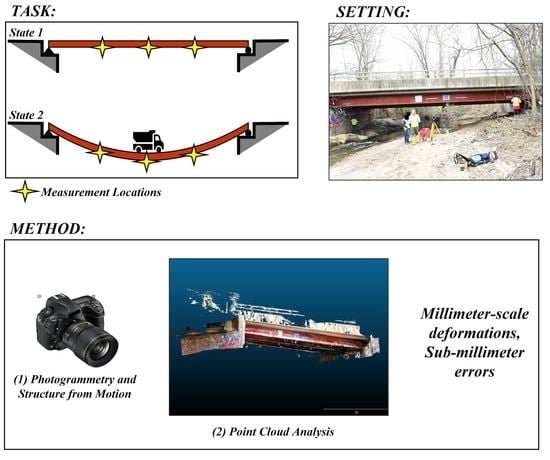
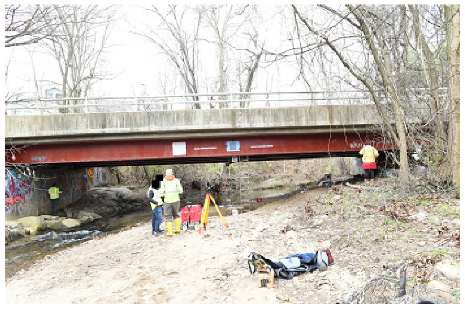
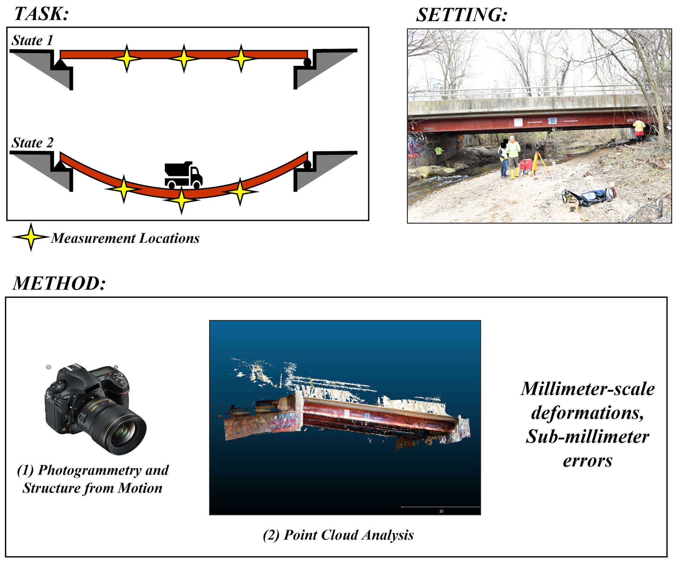
Figure 1 provides an overview of the 3D measurement methodology. In order to quantify deformations, photogrammetric point cloud data are collected from a structure in two states of deformation. The first state is referred to as the “reference” point cloud, representing the unloaded state of the structure, and the second state is referred to as the “compared” point cloud, representing the loaded state of the structure. Prior efforts demonstrated accuracy at the millimeter scale under laboratory conditions for a similar, but simplified, measurement method [36,37,38]. Translating this approach to full-scale field conditions required significant modifications that included specialized image preprocessing, and modifications to the registration algorithm. The overall process is more complex than what is presented in Figure 1, and details are presented in the remainder of this section.

2.1.1. Data Preprocessing

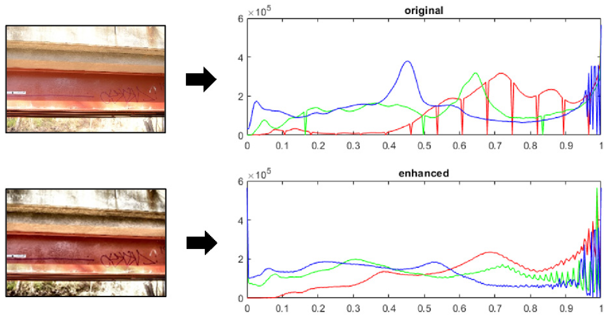
Upon completion of image data collection for both the undeformed and deformed bridge, the digital images must be processed to enhance their brightness and texture. One of the inevitable issues in field photogrammetry is luminance variation between each image due to changes in camera angles and environmental conditions, especially in bright sunlight. SfM is highly dependent on the localized high-contrast regions in the image of an object [39], and histogram equalization results in a more uniform brightness in the images, which enhances the texture of the target and leads to a better 3D reconstruction.

In this work, contrast-limited adaptive histogram equalization (CLAHE) is employed [40]. This algorithm is a specialized form of the adaptive histogram equaliztion (AHE) algorithm that was originally designed to overcome the challenges of performing global histogram equalization on images with a wide range of intensity values across their pixels. However, the AHE algorithm suffers from over-enhancement and noise amplification in regions of the image that have a relatively homogeneous distribution of pixel intensities, a common occurrence for large-scale structures [40,41,42].

CLAHE limits the contrast by clipping and redistributing the histogram of the pixel intensities in the image and therefore avoids the over-enhancement and noise amplification of the AHE algorithm. This step is performed after subdividing the image into several equally sized partitions, and the established clip limit enforces a more uniform contrast across the entirety of the image, thus providing benefit for the SfM process. For additional details on the algorithmic approach for CLAHE, the reader is referred to [43].

It is worth noting that an exhaustive evaluation of multiple image processing algorithms was not conducted. It was shown in other studies that CLAHE is beneficial for 3D point cloud reconstruction by increasing the number of tie points across images and, ultimately, the total number of data points in the point cloud [44,45]. The original motivation for the use of CLAHE resulted from the demonstration of its effectiveness in underwater environments, in which enhancing image visibility and removing artifacts and noise from the images are necessary [46,47]. Thus, because there were similar issues with noise in the images for this work, the authors decided to apply CLAHE to solve non-uniform illumination and brightness problems in the dataset images.

After image processing, the reference and compared point clouds are generated using a dense structure-from-motion algorithm, such as multiview stereo approaches [48,49] or approaches based on semi-global matching [50]. The point clouds are then scaled into a global reference frame that accommodates an effective interpretation of the results for deformation tracking. This scaling is typically achieved using a metric, either through calibration targets placed within a scene or through known dimensions of objects within a point cloud [51]. The experiments in this work employed calibration targets, as will be discussed in Section 3.

After point cloud generation and scaling, the next step is to remove clear outliers in the point cloud. Three-dimensional data points are classified as either inlier or outlier points based on the local neighborhood structure, and follow the approach found in [52]. First, a local neighborhood structure of the k-nearest neighbors is established for each point in the dataset. Next, the average distance, d, from a point to its k local neighbors is computed, and the mean, $\mu$, and standard deviation, $\sigma$, of these distances (across the entirety of the dataset) are determined. Data points are classified as outliers when their average distances, d, to their associated local neighborhoods meet the following condition:

$$d_{outlier}\ge \mu +\alpha \sigma$$

(1)

The values for k and $\alpha$ are determined empirically such that a small percentage of the data points are classified as outliers and can then be deleted from the dataset. The intent of this statistical approach is to delete points that are far away from neighboring data points while still preserving the curvature and local features of the data.

2.1.2. Registration

The geometric registration of the reference and compared point sets is broken into two steps: an approximate manual alignment, followed by a fine alignment that minimizes registration errors. For the first step, the point sets are aligned manually by identifying eight pairs of common points. An important detail of point pair selection is that the common points between the datasets must be in the same location between the two load states of the structure. In other words, no point pairs may be selected on a portion of the structure that deforms to a different spatial location during its loading. As a general rule, point pairs should be located on the wall of the supporting abutments or convenient locations not attached to the bridge that can be captured in the scene with point cloud data. Such locations could include areas on immobile objects such as rock faces or artificially placed fiducial objects. Having selected the point pairs, a transformation is applied to the compared point cloud to roughly align the entirety of the loaded structure into the same globally-scaled 3D space as the unloaded structure represented by the reference point cloud.

Due to noise (defined with respect to point cloud data herein as residuals between the surface represented by the data point and the true surface location) in the data and the limitation of the point pair selection with respect to alignment accuracy, manual alignment is typically not accurate enough for deformation tracking at the millimeter scale. Preliminary manual alignment is critical though, as the algorithms used for fine registration tend to converge to a local optimum. The intent of the manual registration is to set the initial position of the compared point cloud such that the solution to the fine registration algorithm is the global solution.

The fine registration process in this work uses the iterative closest point (ICP) algorithm [35], a point-to-point registration algorithm based on Euclidean distances between the points in the two point clouds (Figure 2). First, the algorithm finds the nearest neighbor point correspondences between the point clouds using kd-tree space partitioning to reduce the search complexity [53]. Given the reference point cloud P, where all points $p\in P$, and the compared point cloud Q, where all points $q\in Q$, the ICP calculates the Euclidean distances of the m correspondences between all points $p_i$ and $q_i$ (denoted as a correspondence pair). ICP then iteratively calculates the 3 × 3 rotation matrix, R, and 3 × 1 translation vector, t, of the registration for the target point cloud, Q, through the minimization of the cost function shown in Equation (2).

$$E(\mathbf{R},\mathbf{t})=\underset{R,t}{arg\; min}\sum _{i=1}^n{\parallel p_i-(\mathbf{R}{q}_i+\mathbf{t})\parallel }_2$$

(2)

Because the ICP minimizes Euclidean distances between point correspondences, it is commonly referred to as point-to-point ICP. A variant of this algorithm, known as point-to-plane ICP [54], seeks to overcome the complications from the unsigned directionality of point-to-point Euclidean distances. This variant can be beneficial in cases where the point sets are representative of planar surfaces. For the point-to-plane version, the Euclidean distances between the point correspondences are projected along the direction of the surface normal vector from the point in the reference point cloud for each correspondence (Figure 3).

As a result, the cost function includes the surface normal vector, $n_i$, for the corresponding point, $p_i$ (Equation (3)).

$$E(\mathbf{R},\mathbf{t})=\underset{R,t}{arg\; min}\sum _{i=1}^m({(p_i-(\mathbf{R}{q}_i+\mathbf{t}))}^T·n_i)$$

(3)

For either point-to-point ICP or point-to-plane ICP, it is not required to have the same number of data points in each point cloud, as the algorithm runs based on the correspondences between nearest neighbors. At the scale of the point clouds used in structural assessment, this is algorithmically beneficial because it is unrealistic to expect the point cloud datasets to have the same number of data points without point set subsampling. However, this characteristic leads to countless correspondence arrangements where one data point will be a nearest neighbor to multiple data points in the opposing point cloud and therefore makes the performance of the registration algorithms sensitive to noise, outliers, and the initial pose from manual registration.

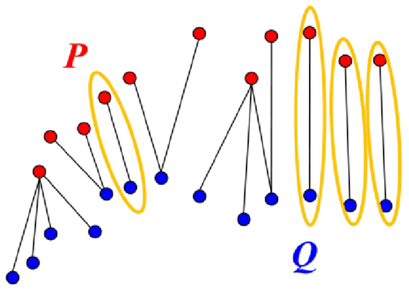
In response to this shortcoming, researchers developed a version of the ICP [55] that adopts characteristics of a generalized Procrustes analysis (GPA). For GPA, point cloud datasets have the same number of points, and the point correspondences are known a priori. The GPA-ICP algorithm mimics this arrangement by only using point correspondences from mutual nearest neighbors before executing the ICP algorithm. A data point $p\in P$ is defined as the mutual nearest neighbor to $q\in Q$ when the nearest neighbor to p in Q is q and the nearest neighbor to q in P is p. Thus, the mutual nearest neighbors have an exclusive nearest neighbor relationship from the remainder of the points in the datasets (Figure 4). Using the mutual nearest neighbors to define the point correspondences for the ICP algorithm results in less sensitivity to outliers at the expense of a higher computational cost.

The version of the algorithm in this work determines the mutual nearest neighbors between the two point sets and runs the ICP algorithm based on these correspondences. After converging to a registration solution, the algorithm then iterates the process by determining a new set of mutual nearest neighbors based on the position of the moving point cloud from the previous iteration. The iterations are continued until a given criteria is met (such as a set number of iterations or a given differential between subsequent transformations).

Other registration algorithms explored for this work included the coherent point drift (CPD) [56] and the normal distributions transform (NDT) [57]. These algorithms are probability-based metrics that use the expectation-maximization algorithm while treating the data points in the compared point cloud treated as centroids of Gaussian mixture models (the approach for the CPD algorithm), or break the datasets into voxels and transform the compared point cloud based on mean and variance of the data locations in each voxel (the approach for the NDT algorithm). However, initial research with these algorithms did not provide sufficiently accurate results and is therefore not discussed further.

2.1.3. Deformation Measurement

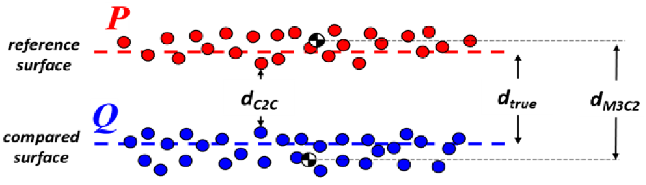
Once the registration step is complete, the deformations of the structure are determined through the comparison of the two sets of point cloud data. The algorithms considered in this work to make these calculations are the direct cloud-to-cloud (C2C) distance [58], the multi-scale model-to-model cloud comparison (M3C2) [59], and a new approach referred to here as direct point-to-point (P2P) distance metric. While there are many techniques that calculate distances from point cloud data to best fit planes and mesh surfaces, the three algorithms in this work directly compare the distances between individual points in the point sets. This limits unquantifiable uncertainties and undesireable data manipulation that implicitly occur when working with a best-fit plane or meshed surface.

The C2C distance metric is based on a form of the directed Hausdorff distance [60]. In this case, the C2C metric computes the Euclidean distance, d, from a given point in the compared point cloud, Q, to its nearest neighbor in the reference point cloud, P (Equation (4)):

$$d(p,Q)=\underset{q\in Q}{min}{\parallel p-q\parallel }_2$$

(4)

In order to speed up the computation, the point clouds are divided into an octree structure such that the nearest neighbor search includes only an immediate neighborhood of octree cells to a given point, p.

Given Equation (4), the C2C metric necessarily suffers in situations where the point densities between the two sets of point cloud data are different, specifically when the point density of the reference cloud is lower than that of the compared cloud. In such cases, there are many reported distance values among data points in the compared point cloud that are calculated from the same nearest neighbor point in the reference point cloud (Figure 5). However, the benefit of this algorithm is that it is fast and direct.

As an alternate to the fast and direct C2C metric, the M3C2 algorithm accounts for the geometry of the point cloud through the incorporation of the surface normal vectors of the reference point cloud, albeit at the expense of higher computational complexity. For a given set of core points, the M3C2 algorithm determines the surface normal vector through an eigen analysis of the corresponding local neighborhood of points. The spatial covariance matrix of the neighborhood is determined (Equation (5)), and then the smallest eigenvector resulting from a singular value decomposition of this covariance matrix provides a good approximation of the surface normal vector.

$$\mathbf{C}=\frac{1}{n}\sum _{i=1}^n(p_i-\overline{p})\otimes (p_i-\overline{p})$$

(5)

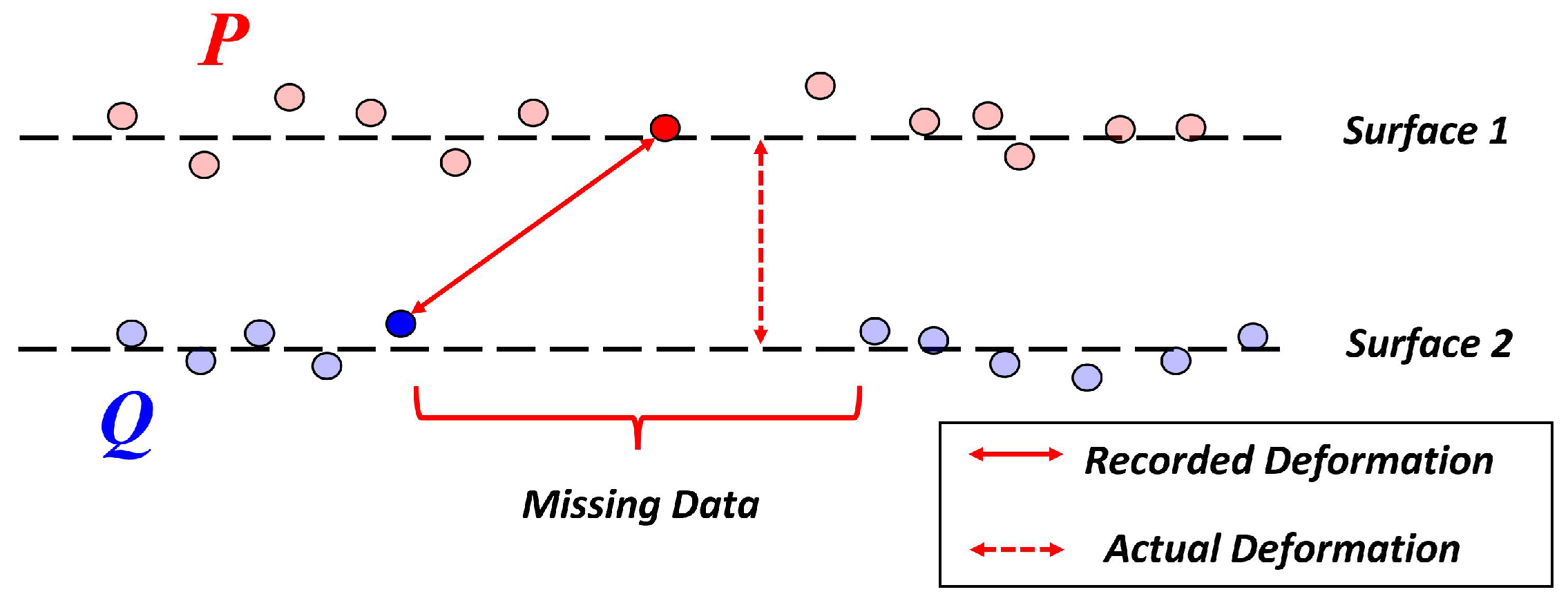
Next, a cylindrical spatial volume at each core point is projected along the surface normal vector. Once this volume is defined, it captures two subsets of data, one from each of the point clouds. The average spatial locations are determined, then the reported distance from the M3C2 algorithm is calculated as the Euclidean distance between the two locations projected on the direction of the calculated surface normal vector for the associated core point. Of note, in cases where the compared point cloud is missing data and no associated data points fall within the spatial volume defined from a given core point, then no M3C2 distance is calculated or reported at that core point (Figure 6).

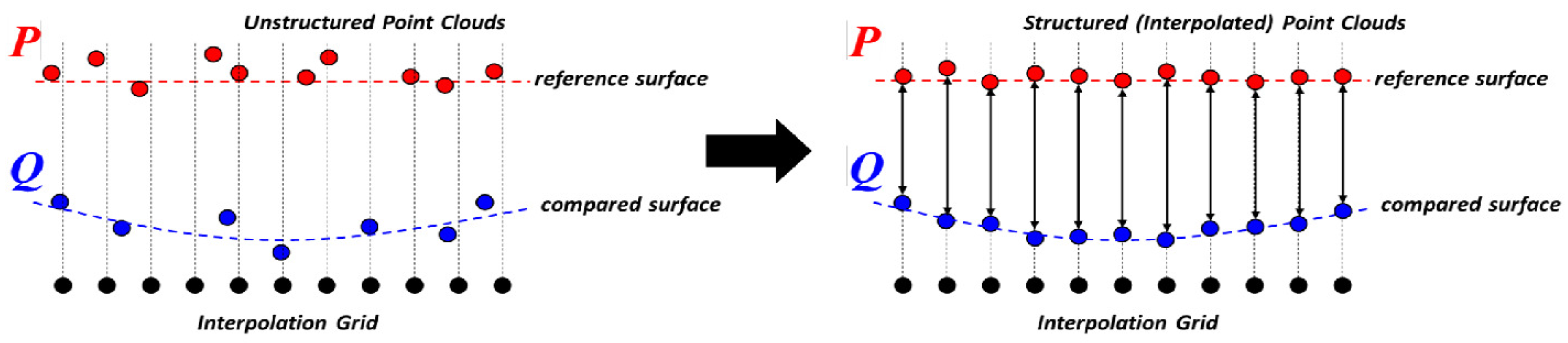
One of the drawbacks of the C2C and M3C2 metrics is that neither algorithm establishes exact correspondences between identical locations on the target structure represented by the point clouds. As a result, the nearest neighbor correspondence for C2C and the mean position correspondence within the core point search volume for M3C2 do not necessarily measure the same exact position on the surface of the structure, leading to measurement error. These algorithms also struggle in instances where data collection is sparse, leading to potential error and an overall lack of confidence in the results. To address this issue, this paper presents a new distance metric, P2P, that establishes point correspondences via interpolation of point cloud data onto a regularized grid that is shared between the two datasets (Figure 7). An interpolation grid is established in the plane that is orthogonal to the direction of primary deformation (i.e., the direction of loading). Gaussian process regression (also known as kriging) [61,62] is conducted on the grid points for each dataset. While other interpolators could also be considered, kriging was selected due to its ability to provide explicit uncertainty quantification, a highly desirable characteristic for structural monitoring applications [63,64].

Once the kriging predictions are made on the orthogonal grid for each dataset, the deformations can be measured through the differences of the kriging predictions. Of note, the kriging process is executed on one-meter-wide local regions of the bottom flange of the outer bridge girder. Results from a cross-validation (not reported here for brevity purposes) support the stationary assumption for the kriging process.

The primary advantage of this approach is that it is robust to locations of missing data (a common occurrence in many practical field applications). Given data point locations in the interpolation grid that lie in the areas of missing data, kriging uses the spatial autocorrelation of the observations in the point cloud to make predictions at these locations to fill in the missing data. While the accuracy of this feature is dependent on the ability to accurately capture and model the spatial autocorrelation, it is preferable in relevant situations.

2.2. Highway Bridge Dataset

The test for the evaluation of this approach was conducted on a highway bridge in New Castle County, Delaware, in 2020. The DE I-213 highway bridge (NBI #1213000) is a privately owned steel girder bridge with a maximum span approximately 21 m long (Figure 8). The targeted structural component for this work was the external steel girder, which was the focus due to its ease of access for data collection. Various load tests for multiple researchers were conducted on the bridge using arrangements of two 20-ton trucks, and this work focused its efforts on two quasi-static load tests. These particular tests were arranged to induce realistically large deflections, although the predicted magnitudes of these tests were predicted to be on the order of only a few millimeters. Experimental validation was provided by installing a string potentiometer at midspan of the target girder. Digital photographs were collected of the unloaded bridge prior to the loads tests to create the reference point cloud.

A Nikon D800E 36-megapixel digital camera with 24 mm lens and a Nikon D850 45-megapixel digital camera with a 50 mm lens were used to collect the digital photographs for raw data. Two photographers worked simultaneously to maximize the number of photographs for the SfM process due to the time constraints for the overall research effort of the day. The data collection approach followed a pattern to ultimately create a set of digital images that would result in one point for every square millimeter of surface area of the bridge girder after completion of the SfM process. This target point cloud density was intended to facilitate capturing deformations at the millimeter scale. The point clouds were created using Agisoft Metashape Professional v 1.5.5 computer software [65]. Settings for the software were determined empirically to produce the best output for the given data. However, the majority were left at default settings after the photographs were screened and discarded if the images were poor in quality.

During data collection, a non-coded fiducial target was placed in the scene, along with coded scale bars accurate to 10 $\mathsf{\mu }$m, near midspan of the outer bridge girder (Figure 9). While the coded scale bars were placed in the scene for scaling the point clouds, the non-coded target was designed to create a convenient coordinate axis system such that the direction of primary deformations was collinear with a selected coordinate axis. It is important to note that these targets were not used during the generation process or registration. Rather, they were used to simplify the reporting and interpretation of experimental results.

Additionally, four coded targets were placed on each bridge support (eight total targets) and these locations served as the reference points for the alignment of the initial pose of the compared point cloud (Figure 9). It should be pointed out that even though these were coded targets, they were not used in any sort of automatic recognition algorithm from the computer software. Instead, these targets were used because they were easy to identify in the point cloud.

2.2.1. Data Preprocessing

Image processing via CLAHE was conducted using MATLAB R2020a [66], and the SfM process was executed using Agisoft Metashape. Images were transformed into the L*a*b* color space and partitioned into 64 tiles for processing, and the normalized lightness value for the clipping limit was set at 0.01 in the L-channel (Figure 10); these settings were determined empirically. Based on the environmental factors in the field and the time constraints for data collection, the ultimate goal of the image processing was to improve image characteristics to enable a better execution of the SfM process. Figure 10 demonstrates the smoothing effects on the three-channel histograms for one of the images, which ultimately results in higher quality point clouds after SfM (results with and without image processing are shown later in Section 3.3).

Once the point clouds were created, they were imported into CloudCompare v2.11.3 [67]. The non-coded fiducial target was used to orient the point cloud such that the longitudinal axis and width of the target bridge girder were oriented in the xy-plane, while the direction of loading and deformation (coincident with the depth of the girder) was oriented along the z-axis. The scale was set based on the average of the calibration distances along two coded scale bars. Statistical outliers were removed based on a local neighborhood size, k, of 30 data points, with points being considered outliers if their nearest neighbor distance was greater than two standard deviations, $\alpha$, away from the mean distance between the neighbors. The use of these parameters generally resulted in slightly less than a 2% reduction in the number of data points. Although this number was slightly larger than what was suggested in [52], it was deemed appropriate due to the expected noise from environmental conditions.

2.2.2. Registration

The manual registration of the point clouds for the initial pose of each of the compared point clouds was conducted in CloudCompare computer software using point-pairs of coded fiducial targets between the compared and reference points clouds.

As mentioned in the previous section, the manual registration is a critical step to set the initial pose of the compared point cloud such that the fine registration algorithms converge to the correct global registration solution. Throughout testing and analysis, small changes in the selection of point pairs between the point clouds resulted in numerous registration solutions for each of the tested fine registration algorithms. As a result, 30 iterations of the manual registration were conducted to enable a cursory statistical evaluation of the fine registration results.

The algorithms for fine registration were executed only on the bridge abutments, as point data in these areas occupied the same physical location between loading scenarios. This approach avoided registration errors from data points in the deformed portion of the structure. The resulting transformation matrix was then applied to the compared point cloud data of the bridge. The fine registration algorithms were executed using MATLAB.

For all tested versions of the ICP algorithm, the full point density of each point cloud was preserved for the fine registration process. While subsampling can speed up the registration process, the total point density was maintained to maximize registration accuracy [34].

For the GPA-ICP algorithm, iterations were executed until the curvature of the compared point cloud demonstrated lower deformations at the quarter spans than mid span. Of note, this step required executing the deformation tracking algorithms after each iteration of the registration.

2.2.3. Deformation Tracking

After registration, the deformation tracking algorithms were conducted on 1-meter-long regions of interest along the bottom flange of the bridge girder. These regions included midspan and each quarter span of the girder, and the bottom flange was used for the calculations because its generally planar shape created a convenient feature for the metrics. The meter-span of each region of interest was chosen to provide enough point comparisons for the distance metrics to statistically evaluate the deformation in the presence of noise and any remaining outliers that may not have been removed during the statistical outlier removal process.

For the C2C metric, the reference point cloud in each region of interest was randomly subsampled such that it would have less than or equal to the same number of data points as the corresponding compared point cloud in the region of interest. This reduced the likelihood of multiple nearest neighbor measurements from the same data point in the reference point cloud. Because the C2C metric uses a Euclidean distance for its calculation, it tends to overestimate the deformations in cases where the one of the point clouds has gaps in the data. In such cases, the distance vector of the point correspondence is off-axis from the primary direction of the deformation (z-axis). As a result, the z-axis components of the C2C distances are reported to better represent the true deformations (Figure 11). It should be pointed out that this approach is not adequate for large gaps in data, in which case other approaches (such as P2P) should be considered. The C2C metric was executed using CloudCompare.

For the M3C2 distance metric, a value of 40 mm was selected for the neighborhood size for surface normal estimation at core points, and this value was slightly over 20 times the size of the smallest eigenvalue, as suggested in [59]. In order to maintain a robust response to local noise, core points were selected from the raw point data with a minimum spacing of 10 mm, spatial volume dimensions of d = 11.3 mm, and a projection length of 10 mm. This cylinder diameter was chosen to result in a surface area roughly equal to 100 mm${}^2$, while the length was chosen empirically to ensure the capture of all of the associated points in the compared point cloud. The M3C2 metric was executed using CloudCompare.

The P2P metric was computed in R v3.6.1 [68,69,70]. For the P2P metric, a uniform interpolation grid was established with over 150,000 points at each region of interest in the xy plane, which, in this case, is orthogonal to the primary direction of loading and deformation. This ensured an approximately equivalent point density to the raw point cloud data. The ordinary kriging process was carried out on a local neighborhood of 100 nearest neighbors for each prediction location, and this number was chosen to balance computational expense with having enough observations to capture the spatial autocorrelation of the data.

2.3. Evaluation and Metrics

2.3.1. Registration Approaches

First, the registration approaches are evaluated based on their sensitivity to the initial manual alignment of the point clouds. Given the tendency for the algorithms to converge to local optima, the transformations of 30 iterations of each fine registration technique are compared in terms of the range and average values of the three translations along the x, y, and z axes and the three Euler angles ($\alpha ,\beta ,\gamma$) around its corresponding axis.

Then, in order to demonstrate the effects of the range of registration solutions, deformation tracking results are compared for each fine registration algorithm. These results are based on the C2C distance metric applied at midspan and each quarter span of the girder. These results are reported in terms of their range and average values. Additionally, a “best case” result is reported from the 30 iterations of each registration. This result is defined, in this context, as the one that most closely matches the reported midspan deflection of the string potentiometer while simultaneously displaying lower values at the quarter spans than midspan. It is recognized that the string-potentiometer has error (as do all sensors), but it is used as the benchmark in this case.

Last, a record of the progression of the GPA-ICP algorithm is presented. Because this algorithm iterates the mutual nearest neighbor determination, the record shows the changes in the reported deformation measurements based on the number of iterations of the algorithm. It is intended to show the computational effort required to report deformation results that demonstrate proper beam curvature at midspan and the quarter spans.

Of note, a single deformation tracking metric (C2C) was chosen for brevity purposes to display the impacts of the translation and rotation ranges from the registration algorithms. The C2C metric was specifically chosen for its simplicity and broad familiarity.

2.3.2. Deformation Tracking Approaches

The deformation calculations for C2C, M3C2, and P2P are compared against the results from string-potentiometer measurements taken at midspan during the load tests. The same evaluation is conducted at the quarter-spans despite the lack of a string potentiometer at those locations. The results are presented as the average and the range of values from the 30 iterations of the given registration algorithm, along with the “best case” result. Similar to the previous evaluation method, a single registration algorithm is chosen for brevity purposes to showcase the performance of the different deformation tracking algorithms. In this case, the ICP algorithm is chosen for its ubiquity across research of point cloud data.

Additionally, a statistical comparison of the deformation tracking algorithms is then performed based on the average results at midspan. Because these values are based on a distribution of measurements from the corresponding region of interest, the standard deviation is used to determine the z-score of a value equivalent to the string-potentiometer measurement. Thus, a lower z-score indicates a higher level of accuracy.

2.3.3. Evaluation of Image Processing Effects

Once the results are presented and the reader has context of the performance of this approach, a comparison is shown that highlights the effects of using the CLAHE image processing algorithm on the digital photographs. Results for midspan deflection, determined by the same initial manual alignment–ICP–C2C workflow, are compared in terms of the z-score corresponding to a sampled value equivalent to the string-potentiometer measurement for the associated load test. For the comparison, one set of results includes the CLAHE image processing step while the other excludes it.

3. Results

3.1. Results of Registration Approaches

Given the methodology presented in Section 2, the registration step serves as a crucial part of the overall process that, if executed ineffectively, has the potential to prevent any sort of reasonable deformation measurement on the millimeter scale. The registration algorithms used in this work were all observed to be dependent on and sensitive to the initial pose of the point cloud data from the manual alignment. This indicates that the registration is a non-convex optimization problem, particularly when considering complex full-scale conditions.

Ideally, the selection of unique point pairs between the datasets should set the compared point cloud into an initial pose that converges to the global optimum registration. Additionally, this global optimum should be found regardless of the choices made by the user for the unique point pairs during manual alignment. However,

Table 1. ICP registration results.

	$\mathit{\alpha }$	$\mathit{\beta }$	$\mathit{\gamma }$	${\mathit{T}}_{\mathit{x}}$	${\mathit{T}}_{\mathit{y}}$	${\mathit{T}}_{\mathit{z}}$
Max	3.0 × 10${}^{-4}$	2.5 × 10${}^{-4}$	−4.7 × 10${}^{-5}$	5.3	0.8	2.0
Avg	1.6 × 10${}^{-4}$	2.3 × 10${}^{-4}$	−5.8 × 10${}^{-5}$	0.1	0.6	1.8
Min	6.4 × 10${}^{-6}$	2.1 × 10${}^{-4}$	−8.0 × 10${}^{-5}$	−1.6	0.4	1.6

,

Table 2. ICP point-to-plane registration results.

	$\mathit{\alpha }$	$\mathit{\beta }$	$\mathit{\gamma }$	${\mathit{T}}_{\mathit{x}}$	${\mathit{T}}_{\mathit{y}}$	${\mathit{T}}_{\mathit{z}}$
Max	3.3 × 10${}^{-3}$	3.4 × 10${}^{-4}$	−3.0 × 10${}^{-4}$	7.0	6.0	3.2
Avg	2.9 × 10${}^{-3}$	2.3 × 10${}^{-4}$	−3.7 × 10${}^{-4}$	1.2	5.2	1.9
Min	2.2 × 10${}^{-3}$	1.3 × 10${}^{-4}$	−5.4 × 10${}^{-4}$	−0.9	3.9	0.8

and

Table 3. GPA-ICP registration results.

	$\mathit{\alpha }$	$\mathit{\beta }$	$\mathit{\gamma }$	${\mathit{T}}_{\mathit{x}}$	${\mathit{T}}_{\mathit{y}}$	${\mathit{T}}_{\mathit{z}}$
Max	2.0 × 10${}^{-4}$	2.9 × 10${}^{-4}$	−2.6 × 10${}^{-4}$	11.0	6.2	2.3
Avg	−3.3 × 10${}^{-4}$	1.6 × 10${}^{-4}$	−4.4 × 10${}^{-4}$	4.3	4.2	1.1
Min	−1.0 × 10${}^{-3}$	2.9 × 10${}^{-5}$	−7.7 × 10${}^{-4}$	2.2	2.9	−0.1

show that the choice of unique point pairs between the two datasets affects the registration results despite the small changes made to the location of the point pair selection.

The tables show the range of values for the Euler angle rotations in radians about each coordinate axis and the translations in millimeters along each respective coordinate axis for all 30 iterations of the given registration algorithm. The results shown are for the first load test. Results for the second load test were similar.

For every registration algorithm, each of the 30 iterations resulted in a slightly different registration solution. This range of values in rotation and translation highlights that the optimization function has many local optima close to the global solution. Concerning the effects of these different solutions on the results of the deformation metrics, the key indicators are the $\beta$ and $T_z$ values, the rotation about the y-axis, and the translation along the z-axis, respectively. While the range of values for the y-axis rotation may seem small, the effects of these values result in large relative rotational errors for large-scale structures, evident in the differences between the deformations at the left and right quarter spans in the deformation tracking step when applied at scale. The quarter span reference measurements for this field test are approximately ten meters apart, and associated rotations about the y-axis on the ${10}^{-4}$ order of magnitude in radians resulted in rotational differences between the quarter span measurements on the order of millimeters. This difference is significant given that the scale of midspan deflection for each load test is only a few millimeters in magnitude.

Likewise, a range of values for translation along the z-axis can be seen across the registration algorithms. Similar to the range of y-axis rotational values, the range of these translations results in large differences among the registration results relative to the millimeter-scaled bridge deformations that were experienced during the load tests.

One of the reasons that the iterations show the range of values for the resulting registration components can be seen in the inherent noise of the point cloud data of the targets. The varying lighting conditions of the field environment during data collection caused the point cloud reconstruction during SfM to result in areas of missing data points and areas with scattered data points that were unable to be isolated and removed during the statistical outlier removal process (Figure 12). This happened regardless of the application of the CLAHE image processing algorithm. The missing and scattered data not only make it difficult to properly select unique point pairs for initial alignment of the point clouds, but also increase the sensitivity of the registration algorithms to finding the correct global registration solution.

When comparing the registration algorithms against each other, a larger range for key rotational ($\beta$) and translation ($T_z$) errors are seen in the ICP point-to-plane and GPA-ICP algorithms when compared to the traditional ICP algorithm. In general, the surface normal vectors for the data points on the bridge supports were oriented along the x-axis, the longitudinal span of the bridge girder. As these points served as the data for the registration algorithms, the increased range in $\beta$ and $T_z$ values likely resulted from the minimization of x-axis component of the Euclidean distances between point correspondences. Likewise, the GPA-ICP algorithm similarly shows a larger range in these values compared to the ICP algorithm, and this relationship likely occurs due to the algorithm finding a unique set of mutual nearest neighbors for each of the 30 registration iterations.

Table 4. Deformation tracking based on ICP.

	Left Quarter	Midspan	Right Quarter
Max	−4.8	$-4.4$	$-4.7$
Avg	$-2.6$	$-2.8$	$-2.3$
Min	$-1.1$	$-1.3$	$-0.3$
Best	$-3.24$	$-3.29$	$-2.69$

,

Table 5. Deformation tracking based on ICP point-to-plane.

	Left Quarter	Midspan	Right Quarter
Max	$-3.7$	$-3.6$	$-3.5$
Avg	$-2.5$	$-2.5$	$-1.8$
Min	$-1.7$	$-1.5$	$-0.3$
Best	$-3.25$	$-3.62$	$-3.49$

and

Table 6. Deformation tracking based on GPA-ICP.

	Left Quarter	Midspan	Right Quarter
Max	$-4.6$	$-4.8$	$-4.6$
Avg	$-2.7$	$-3.2$	$-3.1$
Min	$-1.6$	$-2.1$	$-2.1$
Best	$-3.20$	$-3.42$	$-3.04$

show the deformation tracking results in millimeters at midspan and each quarter span based on the three registration algorithms. These results are for the first load test using the C2C distance metric, and they are in contrast to a −3.5 mm midspan deformation, as measured by the string-potentiometer.

The variations among the registration algorithms resulted in a range of several millimeters at midspan for each method. They also resulted in cases where the rotational errors in the registration are evident, based on a given quarter span deflection being larger than the corresponding midspan and remaining quarter span deflection. It is worth noting that even though the traditional ICP algorithm showed the smallest range in key registration parameters of $\beta$ and $T_z$, it nevertheless shows the largest range for the deformation measurements. This relationship results from translations and rotations along and around the other axes that affect this deformation metric, as it changes the relative location of the noisy data points that were not removed during the outlier removal step. This arrangement then affects the point correspondences for the distance metric calculations.

While the results show close agreement with the potentiometer measurement in the first load test, the second load test results are not as consistent.

Table 7. Second load test averaged deformations.

	Left Quarter	Midspan	Right Quarter
ICP	$-1.32$	$-0.88$	$-2.65$
ICP Point-to-Plane	$-1.63$	$-2.37$	$-6.01$
GPA-ICP	$-2.42$	$-2.83$	$-6.16$

shows the results from the registration algorithms using the C2C distance metric for the second load test. This load test had a field measurement of −2.85 mm of deformation at midspan based on string-potentiometer data. The point cloud created during the second load test was noticeably of lower quality due to time constraints, and this is the most likely cause for the degradation in measurement accuracy. Even though these load tests occurred on the same day under similar lighting conditions, this difference in performance highlights the importance of the data collection phase of the methodology. Note that values at right quarter span for this particular load test are unreliable based on poor-quality local data at the region of interest.

The GPA-ICP algorithm shows promising results for both load tests, but it should be pointed out that the algorithm required multiple iterations to reach a reasonable registration solution (

Table 8. Progression of GPA-ICP algorithm.

Iteration #	Left Quarter	Midspan	Right Quarter
1	−2.85	−4.12	−5.09
10	−2.68	−3.56	−3.98
30	−2.62	−3.30	−3.48
60	−2.65	−3.23	−3.30
90	−2.70	−3.23	−3.22
100	−2.71	−3.22	−3.19

). As the other two versions of the ICP in this work demonstrated convergence to local optima based on the manual alignment, the GPA-ICP avoids this problem through its mutual nearest neighbors approach. The problem with the use of GPA-ICP is that it did not demonstrate convergence to a global solution after a reasonable number of iterations, and the number of iterations of the algorithm for each load test were determined empirically based on the a priori knowledge of the midspan deformation. Further, the algorithm was not executed for a similar number of iterations for each load test, as the first load test required 100 iterations and the second required only 7 iterations.

3.2. Results of Deformation Tracking Approaches

Table 9. C2C results using ICP registration.

	Left Quarter	Midspan	Right Quarter
Max	−4.8	−4.4	−4.7
Avg	−2.6	−2.8	−2.3
Min	−1.1	−1.3	−0.3
Best	−3.24	−3.29	−2.69

,

Table 10. M3C2 results using ICP registration.

	Left Quarter	Midspan	Right Quarter
Max	−6.4	−5.4	−5.4
Avg	−3.8	−3.6	−2.8
Min	−2.0	−1.8	−0.5
Best	−3.66	−3.50	−2.92

and

Table 11. Direct P2P results using ICP registration.

	Left Quarter	Midspan	Right Quarter
Max	−7.7	−6.9	−5.1
Avg	−4.6	−4.6	−2.9
Min	−2.3	−2.5	−0.6
Best	−2.62	−3.57	−2.89

show a comparison of the results for the different deformation tracking algorithms. In order to have a consistent registration method for comparison purposes of the deformation tracking algorithms, this table shows the results using the traditional ICP algorithm only.

A consistent pattern that is demonstrated in these results is that the C2C metric in this scenario measures a lower deformation value than the M3C2 and direct P2P metrics. For such situations that measure generally planar point cloud data with deformations in the orthogonal direction, the C2C metric records the distance within the inner boundaries of the inherent noise of the point cloud datasets, while the M3C2 metric records distances at the mean positions of the point set (Figure 13). Variable lighting conditions in a field environment, as occurred for this field test, are a potential root source of the point noise.

Additionally, the reported values of the C2C metric are based strictly on the z-axis component of the nearest neighbor distances, while the M3C2 metric is based on the orientation of the calculated surface normal vector at the sampled core points. The noise in the data and the likelihood that the deflection was actually off-axis affects the orientation of each surface normal vector, and despite measures taken to ensure that these results are robust to noise, there are undoubtedly normal vectors that are off-axis relative to the direction of deformation. It therefore contributes to an overestimation, albeit very slight, of the distance between measuring locations for the M3C2 algorithm.

It should also be noted that most results for the M3C2 algorithm displayed rotational errors in the deformation tracking based on the ICP registration algorithm, with most of the bias favoring a larger deformation at the left quarter span when compared to midspan. However, this relationship is not universally true for all the registration algorithms. Such results do not necessarily mean that the registration had a rotational error, as there is potential for the large projection length for the search volume of the M3C2 algorithm (set to 10 mm for this work) to capture data noise at the given quarter span location that may not otherwise be present at the other target locations on the bridge girder. Additionally, as the algorithm selects core points based on subsampling of the point cloud, the core points do not represent a unique dataset among the iterations of registration and deformation tracking. Thus, changes to the selected core points can contribute to the bias in the results.

The direct P2P algorithm also displays higher deformations than that of the C2C algorithm. Because the P2P algorithm bases its interpolation results on the spatial autocorrelation of the data, the resulting measurements follow the same pattern as what is seen for the M3C2 metric in Figure 13. However, the performance range (Table 11) and statistical evaluation (

Table 12. Statistical evaluation of deformation tracking.

	Midspan	Std Deviation	Z-Score
C2C	−2.8	2.8	0.25
M3C2	−3.6	2.5	0.03
Direct P2P	−4.6	3.3	0.32

) of the P2P algorithm indicates that it provides a satisfactory performance, even though the other metrics appear to have results closer to the benchmark for this dataset.

Table 12 shows the average midspan deformation measurement in millimeters for all 30 registration iterations using the ICP. The reported standard deviations are determined from these iterations, and the z-score is determined based on an observation value equivalent to the string-potentiometer measurement (−3.5 mm).

Given the demonstrated performance and underlying potential of the P2P algorithm, it serves as a satisfactory alternative to the C2C and M3C2 algorithms in instances where there are gaps in the data. However, it is not the intention to communicate that it will work in all cases of missing data. Sparse data that do not have enough observations to adequately capture the spatial autocorrelation of the point cloud dataset will ultimately negate any benefit for using the P2P algorithm. Figure 14 provides an example of missing data where the P2P algorithm did not perform well (nor did the C2C or M3C2 algorithms, for that matter). This figure highlights the right quarter span target area (Figure 14a) where the point cloud should appear similar to how it appears for the first load test (Figure 14b), but instead ends up being very sparse for the second load test (Figure 14c). These data are sparse enough that none of the deformation tracking algorithms could provide a reasonable result.

3.3. Results of Image Processing

Previous iterations of the methodology shown in Section 2 were executed without image processing. Preliminary measurement results without the application of the CLAHE algorithm had much larger relative errors than those point clouds that had been preprocessed for histogram equalization. This result suggests that the quality of the point clouds plays a critical role in measurement accuracy, a result that was not observed in previous laboratory-scale studies [16].

Table 13. Comparison of relative errors based on CLAHE implementation.

	C2C Midspan	String-Potentiometer	Relative Error
with CLAHE	−2.75	−3.5	−21%
w/o CLAHE	−0.98	−3.5	−72%

demonstrates the benefits of using this algorithm on the raw image data for this particular dataset. The results are based on one iteration each of the research approach (one with and one without CLAHE) that used the same selected point pairs for manual registration, the ICP fine registration algorithm, and the C2C deformation tracking algorithm. The change in relative error is not meant to insinuate that the CLAHE algorithm will universally improve the final results, but it is meant to highlight that point cloud quality is an essential factor for proper execution of the research approach. Units for deformations in Table 13 are millimeters.

4. Discussion

A methodology was presented that considered several critical aspects of the measurement process that included efforts in image processing, scaling, and orientation of point clouds, registration, and deformation measurements. An exhaustive evaluation of the registration process through the implementation of registration algorithms was conducted. The results demonstrated that this step of the methodology is a non-convex optimization problem, and small differences in the initial manual alignment of the point clouds can lead to a wide range of registration solutions and inconsistencies in deformation measurements. The recommended way to avoid this is to implement an approach for the manual alignment and initialization of the registration algorithms that is as accurate and repeatable as possible.

For measuring the deformations, this research investigated the C2C and M3C2 distance metrics, and introduced the direct P2P distance metric, which employs Gaussian process regression to interpolate the point cloud. The evaluation of these techniques showed that, in general, the C2C metric underestimated the deformation while the M3C2 and direct P2P metrics overestimated the deformation when compared to the field measurements recorded by the string-potentiometer. Even though these metrics did not consistently agree with the field measurements, statistical evaluation demonstrated that they were able to capture the benchmark midspan deformation within one standard deviation of the mean reported value. These distance metrics demonstrated applicability to measuring changes between planar surfaces that deform along a known coordinate axis direction. In cases where structural deformations are less predictable, or in other scenarios where changes between point cloud data are not understood a priori, other approaches for deformation tracking should be considered. In general, these approaches should consider deformations in all principal directions as opposed to a singular direction, as demonstrated in this work.

This research did not conduct an exhaustive evaluation of image processing techniques for data preprocessing. The inclusion of the CLAHE algorithm made a noticeable and satisfactory improvement to the results, and it was not the intention of the authors to optimize the image processing step. However, it is important to recognize that the quality of the point cloud data, improved in this case by CLAHE, is vital for successful implementation of the registration and deformation tracking algorithms.

It is important to highlight that this approach is limited to scenarios where geometric changes of the target structure are the indicators of structural performance or behavior. In this context, the presented approach is not necessarily applicable for such applications as crack detection. Additionally, because the approach focuses on geometric changes between point clouds in different loading scenarios, it must be applied in static loading conditions. While this has connotations of use in long-term structural health monitoring scenarios to identify problems from fatigue or settlement, it also means that it is not appropriate for dynamic loading situations intent on monitoring the vibratory response of a structure.

5. Conclusions

The purpose of this work was to present a case study on the use of photogrammetric point cloud analysis for static load testing and deformation tracking of a highway bridge in Delaware, USA. This case study is significant because it used remotely sensed point cloud data to measure 3D bridge deformations at the millimeter scale in a field environment, and it stands in contrast to other research efforts that either used laser scanning for data collection or worked with laboratory or synthetic datasets. This approach to deformation tracking shows promise for continued research and future implementation as there is a continually growing body of research looking for more efficient ways for structural assessment that do not rely on installed sensor arrays.

Additional research efforts in deformation tracking of highway bridges from photogrammetry point cloud data can evaluate operational practices to support point cloud registration. This approach could include the use of natural and geometric objects placed at strategic locations in the scene to support the manual alignment of the point clouds. Additionally, implementation of these algorithms against point cloud data of other bridges (i.e., truss, suspension, or other multi-span bridges) could strengthen the merit of this work. Other future research could include efforts to apply these algorithms, or variations of them, to structural systems with higher curvature.

References

1. Lucas, J.; Via, C.E.; Brown, M.C.; Sharp, S.R.; Lane, D.S. Structural Load Testing and Flexure Analysis of the Route 701 Bridge in Louisa County, Virginia; Technical Report; Virginia Transportation Research Council: Charlottesville, VA, USA, 2004. [Google Scholar]
2. Hag-Elsafi, O.; Kunin, J. Load Testing for Bridge Rating: Route 22 over Swamp River; Technical Report FHWA/NY/SR-06/144; Transportation Research and Development Bureau: Albany, NY, USA, 2006.
3. Gattulli, V.; Lepidi, M.; Potenza, F. Dynamic Testing and Health Monitoring of Historic and Modern Civil Structures in Italy. Struct. Monit. Maint. 2016, 3, 71–90. [Google Scholar] [CrossRef]
4. Amies, A.C.; Pretty, C.G.; Rodgers, G.W.; Chase, J.G. Shake Table Testing of a Radar-Based Structural Health Monitoring Method. In Proceedings of the 2018 14th IEEE/ASME International Conference on Mechatronic and Embedded Systems and Applications (MESA), Oulu, Finland, 2–4 July 2018; pp. 1–6. [Google Scholar] [CrossRef]
5. Gueguen, P.; Jolivet, V.; Michel, C.; Schveitzer, A.S. Comparison of Velocimeter and Coherent Lidar Measurements for Building Frequency Assessment. Bull. Earthq. Eng. 2010, 8, 327–338. [Google Scholar] [CrossRef]
6. Farahani, R.V.; Penumadu, D. Damage Identification of a Full-Scale Five-Girder Bridge Using Time-Series Analysis of Vibration Data. Eng. Struct. 2016, 115, 129–139. [Google Scholar] [CrossRef]
7. Adams, A.; Galindez, N.; Hopper, T.; Murphy, T.; Ritchie, P.; Storlie, V.; Weisman, J. Manual for Refined Analysis in Bridge Design and Evaluation; Technical Report FHWA-HIF-18-046; US Department of Transportation Federal Highway Administration: Washington, DC, USA, 2019.
8. Xu, Y.; Brownjohn, J.M.W.; Hester, D.; Koo, K.Y. Dynamic Displacement Measurement of a Long-Span Bridge Using Vision-based System. In Proceedings of the 8th European Workshop On Structural Health Monitoring (EWSHM 2016), Bilbao, Spain, 5–8 July 2016; p. 11. [Google Scholar]
9. Tang, Y.; Zhu, M.; Chen, Z.; Wu, C.; Chen, B.; Li, C.; Li, L. Seismic Performance Evaluation of Recycled Aggregate Concrete-Filled Steel Tubular Columns with Field Strain Detected via a Novel Mark-Free Vision Method. Structures 2022, 37, 426–441. [Google Scholar] [CrossRef]
10. Chen, M.; Tang, Y.; Zou, X.; Huang, K.; Li, L.; He, Y. High-Accuracy Multi-Camera Reconstruction Enhanced by Adaptive Point Cloud Correction Algorithm. Opt. Lasers Eng. 2019, 122, 170–183. [Google Scholar] [CrossRef]
11. Feng, D.; Feng, M.; Ozer, E.; Fukuda, Y. A Vision-Based Sensor for Noncontact Structural Displacement Measurement. Sensors 2015, 15, 16557–16575. [Google Scholar] [CrossRef]
12. Sun, D.; Roth, S.; Black, M.J. Secrets of Optical Flow Estimation and Their Principles. In Proceedings of the 2010 IEEE Computer Society Conference on Computer Vision and Pattern Recognition, San Francisco, CA, USA, 13–18 June 2010; pp. 2432–2439. [Google Scholar] [CrossRef] [Green Version]
13. Khuc, T.; Catbas, F.N. Computer Vision-Based Displacement and Vibration Monitoring without Using Physical Target on Structures. Struct. Infrastruct. Eng. 2017, 13, 505–516. [Google Scholar] [CrossRef]
14. Xu, Y.; Brownjohn, J.M.; Huseynov, F. Accurate Deformation Monitoring on Bridge Structures Using a Cost-Effective Sensing System Combined with a Camera and Accelerometers: Case Study. J. Bridge Eng. 2019, 24, 05018014. [Google Scholar] [CrossRef] [Green Version]
15. Xu, Y.; Brownjohn, J.; Kong, D. A Non-Contact Vision-Based System for Multipoint Displacement Monitoring in a Cable-Stayed Footbridge. Struct. Control Health Monit. 2018, 25, e2155. [Google Scholar] [CrossRef] [Green Version]
16. Jafari, B.; Khaloo, A.; Lattanzi, D. Deformation Tracking in 3D Point Clouds Via Statistical Sampling of Direct Cloud-to-Cloud Distances. J. Nondestruct. Eval. 2017, 36, 65. [Google Scholar] [CrossRef]
17. Erdélyi, J.; Kopáčik, A.; Lipták, I.; Kyrinovič, P. Automation of Point Cloud Processing to Increase the Deformation Monitoring Accuracy. Appl. Geomat. 2017, 9, 105–113. [Google Scholar] [CrossRef]
18. Riveiro, B.; Jauregui, D.; Arias, P.; Armesto, J.; Jiang, R. An Innovative Method for Remote Measurement of Minimum Vertical Underclearance in Routine Bridge Inspection. Autom. Constr. 2012, 25, 34–40. [Google Scholar] [CrossRef]
19. Riveiro, B.; González-Jorge, H.; Varela, M.; Jauregui, D. Validation of Terrestrial Laser Scanning and Photogrammetry Techniques for the Measurement of Vertical Underclearance and Beam Geometry in Structural Inspection of Bridges. Measurement 2013, 46, 784–794. [Google Scholar] [CrossRef]
20. Liu, M.; Sun, X.; Wang, Y.; Shao, Y.; You, Y. Deformation Measurement of Highway Bridge Head Based on Mobile TLS Data. IEEE Access 2020, 8, 85605–85615. [Google Scholar] [CrossRef]
21. Oskouie, P.; Becerik-Gerber, B.; Soibelman, L. Automated Measurement of Highway Retaining Wall Displacements Using Terrestrial Laser Scanners. Autom. Constr. 2016, 65, 86–101. [Google Scholar] [CrossRef]
22. Ye, C.; Acikgoz, S.; Pendrigh, S.; Riley, E.; DeJong, M. Mapping Deformations and Inferring Movements of Masonry Arch Bridges Using Point Cloud Data. Eng. Struct. 2018, 173, 530–545. [Google Scholar] [CrossRef]
23. Cabaleiro, M.; Riveiro, B.; Conde, B.; Sánchez-Rodríguez, A. A Case Study of Measurements of Deformations Due to Different Loads in Pieces Less than 1 m from Lidar Data. Measurement 2020, 151, 107196. [Google Scholar] [CrossRef]
24. Ziolkowski, P.; Szulwic, J.; Miskiewicz, M. Deformation Analysis of a Composite Bridge during Proof Loading Using Point Cloud Processing. Sensors 2018, 18, 4332. [Google Scholar] [CrossRef] [Green Version]
25. Liu, Y.; Kong, D.; Zhao, D.; Gong, X.; Han, G. A Point Cloud Registration Algorithm Based on Feature Extraction and Matching. Math. Probl. Eng. 2018, 2018, 7352691. [Google Scholar] [CrossRef] [Green Version]
26. Yang, H.; Shi, J.; Carlone, L. TEASER: Fast and Certifiable Point Cloud Registration. IEEE Trans. Robot. 2020, 37, 314–333. [Google Scholar] [CrossRef]
27. Yang, J.; Cao, Z.; Zhang, Q. A Fast and Robust Local Descriptor for 3D Point Cloud Registration. Inf. Sci. 2016, 346–347, 163–179. [Google Scholar] [CrossRef]
28. Korn, M.; Holzkothen, M.; Pauli, J. Color Supported Generalized-ICP. In Proceedings of the 2014 International Conference on Computer Vision Theory and Applications (VISAPP), Lisbon, Portugal, 5–8 January 2014; pp. 592–599. [Google Scholar]
29. Park, J.; Zhou, Q.Y.; Koltun, V. Colored Point Cloud Registration Revisited. In Proceedings of the 2017 IEEE International Conference on Computer Vision (ICCV), Venice, Italy, 22–29 October 2017; pp. 143–152. [Google Scholar] [CrossRef]
30. Serafin, J.; Grisetti, G. NICP: Dense Normal Based Point Cloud Registration. In Proceedings of the 2015 IEEE/RSJ International Conference on Intelligent Robots and Systems (IROS), Hamburg, Germany, 28 September–2 October2015; pp. 742–749. [Google Scholar] [CrossRef] [Green Version]
31. Aoki, Y.; Goforth, H.; Srivatsan, R.A.; Lucey, S. PointNetLK: Robust & Efficient Point Cloud Registration Using PointNet. In Proceedings of the 2019 IEEE/CVF Conference on Computer Vision and Pattern Recognition (CVPR), Long Beach, CA, USA, 16–20 June 2019; pp. 7156–7165. [Google Scholar] [CrossRef] [Green Version]
32. Wang, Y.; Solomon, J. Deep Closest Point: Learning Representations for Point Cloud Registration. In Proceedings of the 2019 IEEE/CVF International Conference on Computer Vision (ICCV), Seoul, Korea, 27–28 October 2019; pp. 3522–3531. [Google Scholar] [CrossRef] [Green Version]
33. Wang, Y.; Solomon, J.M. PRNet: Self-Supervised Learning for Partial-to-Partial Registration. arXiv 2019, arXiv:1910.12240. [Google Scholar]
34. Dong, Z.; Liang, F.; Yang, B.; Xu, Y.; Zang, Y.; Li, J.; Wang, Y.; Dai, W.; Fan, H.; Hyyppä, J.; et al. Registration of Large-Scale Terrestrial Laser Scanner Point Clouds: A Review and Benchmark. ISPRS J. Photogramm. Remote Sens. 2020, 163, 327–342. [Google Scholar] [CrossRef]
35. Besl, P.J.; McKay, N.D. Method for Registration of 3-D Shapes. In Proceedings of the Fifth International Conference on Advanced Robotics: ‘91 ICAR, Pisa, Italy, 19–22 June 1991; pp. 586–606. [Google Scholar] [CrossRef]
36. Khaloo, A.; Lattanzi, D. Hierarchical Dense Structure-from-Motion Reconstructions for Infrastructure Condition Assessment. J. Comput. Civ. Eng. 2017, 31, 04016047. [Google Scholar] [CrossRef]
37. Sapirstein, P. Accurate Measurement with Photogrammetry at Large Sites. J. Archaeol. Sci. 2016, 66, 137–145. [Google Scholar] [CrossRef]
38. Verma, A.K.; Bourke, M.C. A Method Based on Structure-from-Motion Photogrammetry to Generate Sub-Millimetre-Resolution Digital Elevation Models for Investigating Rock Breakdown Features. Earth Surf. Dyn. 2019, 7, 45–66. [Google Scholar] [CrossRef] [Green Version]
39. Momtaz Dargahi, M.; Khaloo, A.; Lattanzi, D. Color-Space Analytics for Damage Detection in 3D Point Clouds. Struct. Infrastruct. Eng. 2021, 18, 775–788. [Google Scholar] [CrossRef]
40. Pizer, S.; Johnston, R.; Ericksen, J.; Yankaskas, B.; Muller, K. Contrast-Limited Adaptive Histogram Equalization: Speed and Effectiveness. In Proceedings of the First Conference on Visualization in Biomedical Computing, Atlanta, GA, USA, 22–25 May 1990; pp. 337–345. [Google Scholar] [CrossRef]
41. Pirie, C.; Moreno-Garcia, C.F. Image Pre-processing and Segmentation for Real-Time Subsea Corrosion Inspection. In Proceedings of the 22nd Enginering Applications of Neural Networks Conference (EANN2021), Halkidiki, Greece, 25–27 June 2021; Iliadis, L., Macintyre, J., Jayne, C., Pimenidis, E., Eds.; Springer International Publishing: Cham, Switzerland, 2021; Volume 3, pp. 220–231. [Google Scholar] [CrossRef]
42. Unal, B.; Akoglu, A. Resource Efficient Real-Time Processing of Contrast Limited Adaptive Histogram Equalization. In Proceedings of the 2016 26th International Conference on Field Programmable Logic and Applications (FPL), Lausanne, Switzerland, 29 August–2 September 2016; pp. 1–8. [Google Scholar] [CrossRef]
43. Reza, A.M. Realization of the Contrast Limited Adaptive Histogram Equalization (CLAHE) for Real-Time Image Enhancement. J. VLSI Signal Process. Syst. Signal Image Video Technol. 2004, 38, 35–44. [Google Scholar] [CrossRef]
44. Malinverni, E.S.; Cerrano, C.; Pantaleo, U.; Andreola, C.; Paolanti, M.; Chiappini, S.; Pierdicca, R. Image enhancement comparison to improve underwater cultural heritage survey. IOP Conf. Ser. Mater. Sci. Eng. 2020, 949, 012102. [Google Scholar] [CrossRef]
45. Moon, D.; Lee, K.; Ko, H.; Kwon, S.; Lee, S.; Song, J. Analysis of Accuracy Factor and Pre-Processing Methodology of Image Compensation for 3D Reconstruction Using 2D Image Obtained from Unmanned Aerial Vehicle (UAV). J. Asian Archit. Build. Eng. 2021, 1–14. [Google Scholar] [CrossRef]
46. Fabio, O.; Fabjan, K.; Dario, L.R.; Jacopo, A.; Stefano, C. Performance Evaluation of a Low-Cost Stereo Vision System for Underwater Object Detection. IFAC Proc. Vol. 2014, 47, 3388–3394. [Google Scholar] [CrossRef] [Green Version]
47. Chung, D.; Kim, J. Pose Estimation Considering an Uncertainty Model of Stereo Vision for In-Water Ship Hull Inspection. IFAC-PapersOnLine 2018, 51, 400–405. [Google Scholar] [CrossRef]
48. Pollefeys, M.; Van Gool, L.; Vergauwen, M.; Verbiest, F.; Cornelis, K.; Tops, J.; Koch, R. Visual Modeling with a Hand-Held Camera. Int. J. Comput. Vis. 2004, 59, 207–232. [Google Scholar] [CrossRef]
49. Furukawa, Y.; Ponce, J. Accurate, Dense, and Robust Multiview Stereopsis. IEEE Trans. Pattern Anal. Mach. Intell. 2009, 32, 1362–1376. [Google Scholar] [CrossRef]
50. Hirschmuller, H. Stereo Processing by Semiglobal Matching and Mutual Information. IEEE Trans. Pattern Anal. Mach. Intell. 2008, 30, 328–341. [Google Scholar] [CrossRef]
51. Mathews, A.; Jensen, J. Visualizing and Quantifying Vineyard Canopy LAI Using an Unmanned Aerial Vehicle (UAV) Collected High Density Structure from Motion Point Cloud. Remote Sens. 2013, 5, 2164–2183. [Google Scholar] [CrossRef] [Green Version]
52. Rusu, R.B.; Marton, Z.C.; Blodow, N.; Dolha, M.; Beetz, M. Towards 3D Point Cloud Based Object Maps for Household Environments. Robot. Auton. Syst. 2008, 56, 927–941. [Google Scholar] [CrossRef]
53. Friedman, J.H.; Bentley, J.L.; Finkel, R.A. An Algorithm for Finding Best Matches in Logarithmic Expected Time. ACM Trans. Math. Softw. 1977, 3, 209–226. [Google Scholar] [CrossRef]
54. Chen, Y.; Medioni, G. Object Modelling by Registration of Multiple Range Images. Image Vis. Comput. 1992, 10, 145–155. [Google Scholar] [CrossRef]
55. Toldo, R.; Beinat, A.; Crosilla, F. Global Registration of Multiple Point Clouds Embedding the Generalized Procrustes Analysis into an ICP Framework. In Proceedings of the 5th International Symposium on 3D Data Processing, Visualization and Transmission (3DPVT), Chapel Hill, NC, USA, 14–16 June 2006; p. 9. [Google Scholar]
56. Myronenko, A.; Song, X. Point Set Registration: Coherent Point Drift. IEEE Trans. Pattern Anal. Mach. Intell. 2010, 32, 2262–2275. [Google Scholar] [CrossRef] [Green Version]
57. Biber, P.; Strasser, W. The Normal Distributions Transform: A New Approach to Laser Scan Matching. In Proceedings of the 2003 IEEE/RSJ International Conference on Intelligent Robots and Systems (IROS 2003) (Cat. No.03CH37453), Las Vegas, NV, USA, 27–31 October 2003; Volume 3, pp. 2743–2748. [Google Scholar] [CrossRef]
58. Girardeau-Montaut, D.; Roux, M.; Marc, R.; Thibault, G. Change Detection on Points Cloud Data Acquired with a Ground Laser Scanner; International Archives of Photogrammetry, Remote Sensing, and Spatial Information Series; ISPRS: Enschede, The Netherlands, 2005; pp. 30–35. [Google Scholar]
59. Lague, D.; Brodu, N.; Leroux, J. Accurate 3D Comparison of Complex Topography with Terrestrial Laser Scanner: Application to the Rangitikei Canyon (N-Z). ISPRS J. Photogramm. Remote Sens. 2013, 82, 10–26. [Google Scholar] [CrossRef] [Green Version]
60. Huttenlocher, D.; Klanderman, G.; Rucklidge, W. Comparing Images Using the Hausdorff Distance. IEEE Trans. Pattern Anal. Mach. Intell. 1993, 15, 850–863. [Google Scholar] [CrossRef] [Green Version]
61. Bailey, T.C.; Gatrell, A.C. Interactive Spatial Data Analysis, pap/dskt ed.; Routledge: London, UK, 1995. [Google Scholar]
62. Cressie, N.A.C. Statistics for Spatial Data, rev. ed.; Wiley Series in Probability and Mathematical Statistics; Wiley: New York, NY, USA, 1993. [Google Scholar]
63. Olivier, A.; Giovanis, D.G.; Aakash, B.; Chauhan, M.; Vandanapu, L.; Shields, M.D. UQpy: A General Purpose Python Package and Development Environment for Uncertainty Quantification. J. Comput. Sci. 2020, 47, 101204. [Google Scholar] [CrossRef]
64. Olivier, A.; Shields, M.D.; Graham-Brady, L. Bayesian Neural Networks for Uncertainty Quantification in Data-Driven Materials Modeling. Comput. Methods Appl. Mech. Eng. 2021, 386, 114079. [Google Scholar] [CrossRef]
65. Agisoft Metashape User Manual: Professional Edition, Version 1.5; Agisoft LLC: St. Petersburg, Russia, 2019.
66. MATLAB. Version 9.8 (R2020a); Mathworks: Natick, MA, USA, 2020.
67. CloudCompare. CloudCompare Version 2.6.1 User Manual. 2015. Available online: http://www.danielgm.net/cc (accessed on 20 April 2022).
68. R Core Team. R: A Language and Environment for Statistical Computing; R Foundation for Statistical Computing: Vienna, Austria, 2019. [Google Scholar]
69. Pebesma, E.J. Multivariable Geostatistics in S: The Gstat Package. Comput. Geosci. 2004, 30, 683–691. [Google Scholar] [CrossRef]
70. Pebesma, E.; Bivand, R.S. Classes and Methods for Spatial Data: The Sp Package. 2005. Available online: https://cran.r-project.org/web/packages/sp/index.html (accessed on 20 April 2022).
Figure 1. Overview of the methodology.
Remotesensing 14 02767 g001
Figure 2. Example of point correspondences between point clouds P and Q.
Remotesensing 14 02767 g002
Figure 3. Demonstration of point-to-plane ICP. Dashed line shows the point correspondence and the solid line shows the projection along the surface normal vector.
Remotesensing 14 02767 g003
Figure 4. Mutual nearest neighbor correspondences for GPA-ICP are circled.
Remotesensing 14 02767 g004
Figure 5. Comparison of nearest neighbor correspondences under differing point cloud densities. In (a), the reference point cloud has a higher density than the compared point cloud. The figure in (b) is the opposite.
Remotesensing 14 02767 g005
Figure 6. Execution of M3C2 algorithm.
Remotesensing 14 02767 g006
Figure 7. P2P distance metric algorithm.
Remotesensing 14 02767 g007
Figure 8. Delaware I-213 bridge.
Remotesensing 14 02767 g008
Figure 9. Placement of fiducial elements.
Remotesensing 14 02767 g009
Figure 10. Images before (top) and after (bottom) image processing using the CLAHE algorithm. The three-chanel histograms are to the right.
Remotesensing 14 02767 g010
Figure 11. C2C algorithm performance in areas of missing data.
Remotesensing 14 02767 g011
Figure 12. Point cloud data of a registration target.
Remotesensing 14 02767 g012
Figure 13. Example disposition of point cloud noise that can lead to disagreement in deformation tracking algorithms.
Remotesensing 14 02767 g013
Figure 14. Example of missing point data located at (a) right quarter span. Part (b) shows the results for the first load test, while part (c) shows the results for the second load test.
Remotesensing 14 02767 g014