
Continuous Land Cover Change Detection in a Critically Endangered Shrubland Ecosystem Using Neural Networks


Abstract
:1. Introduction
2. Materials and Methods
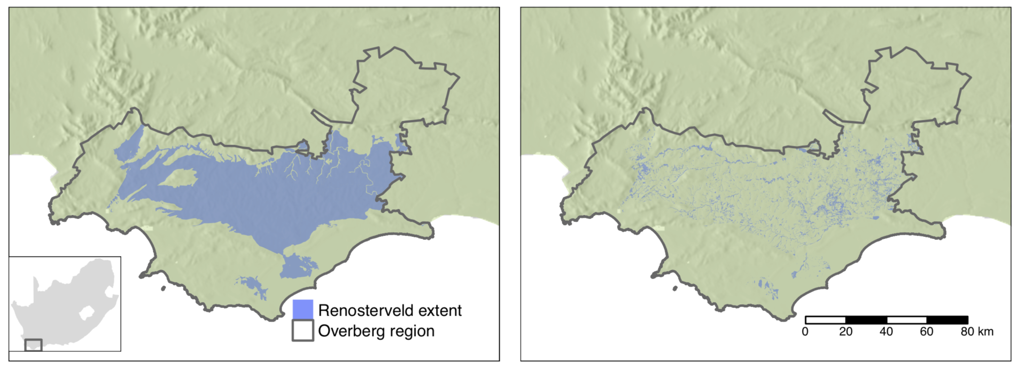
2.1. Study Region
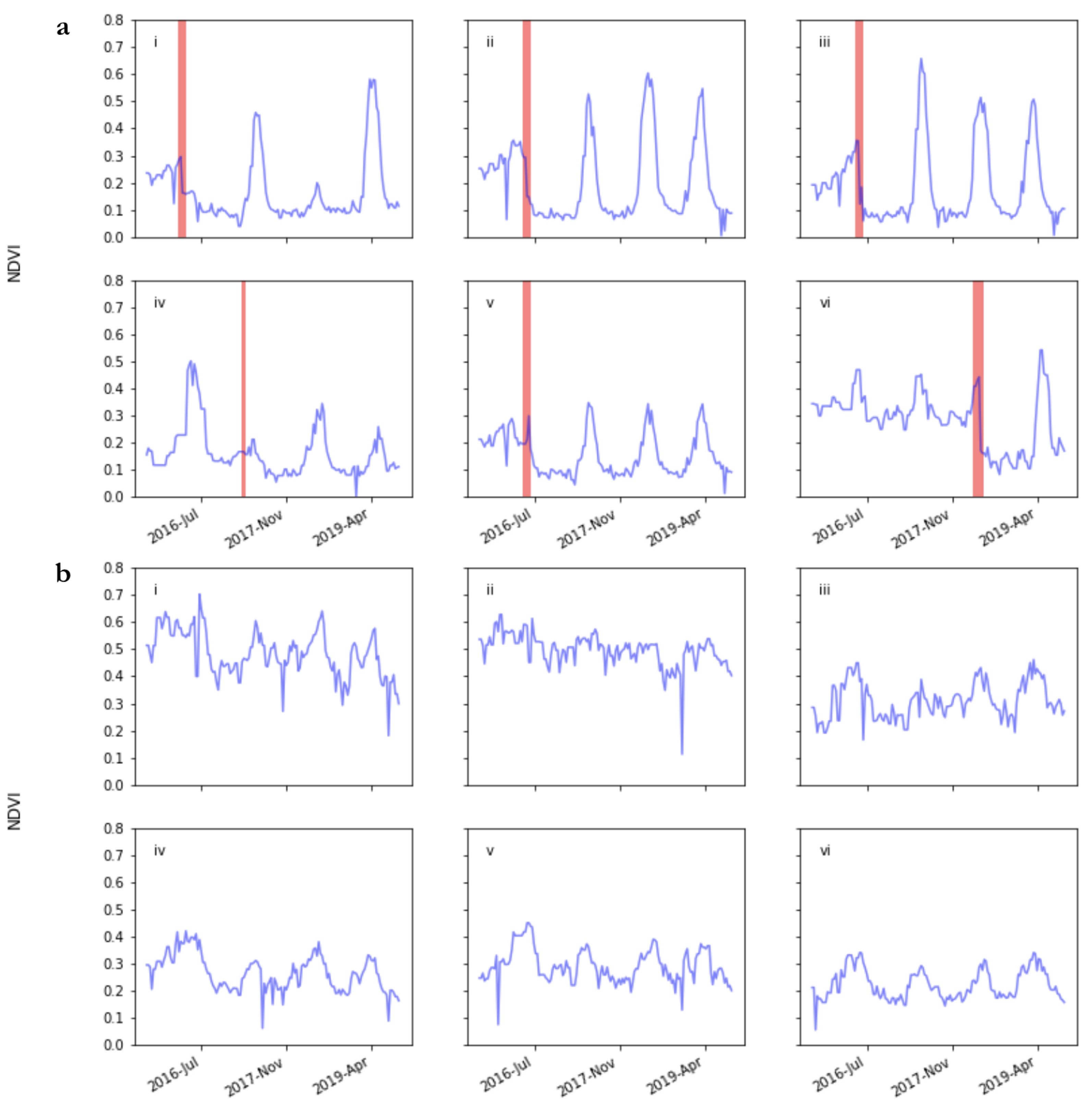
2.2. Land Cover Change Events
2.3. Sentinel 2 Time Series
2.4. Data Labelling
2.5. Models
2.5.1. TempCNN
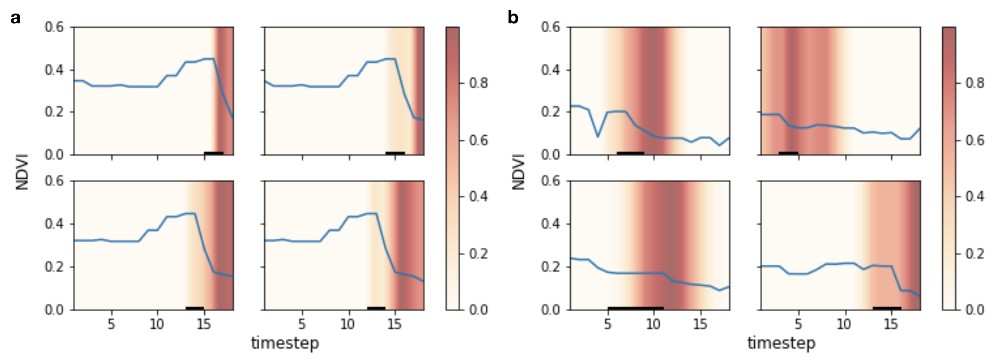
2.5.2. Transformer
2.6. Model Fitting
2.7. Trend Analysis Comparison
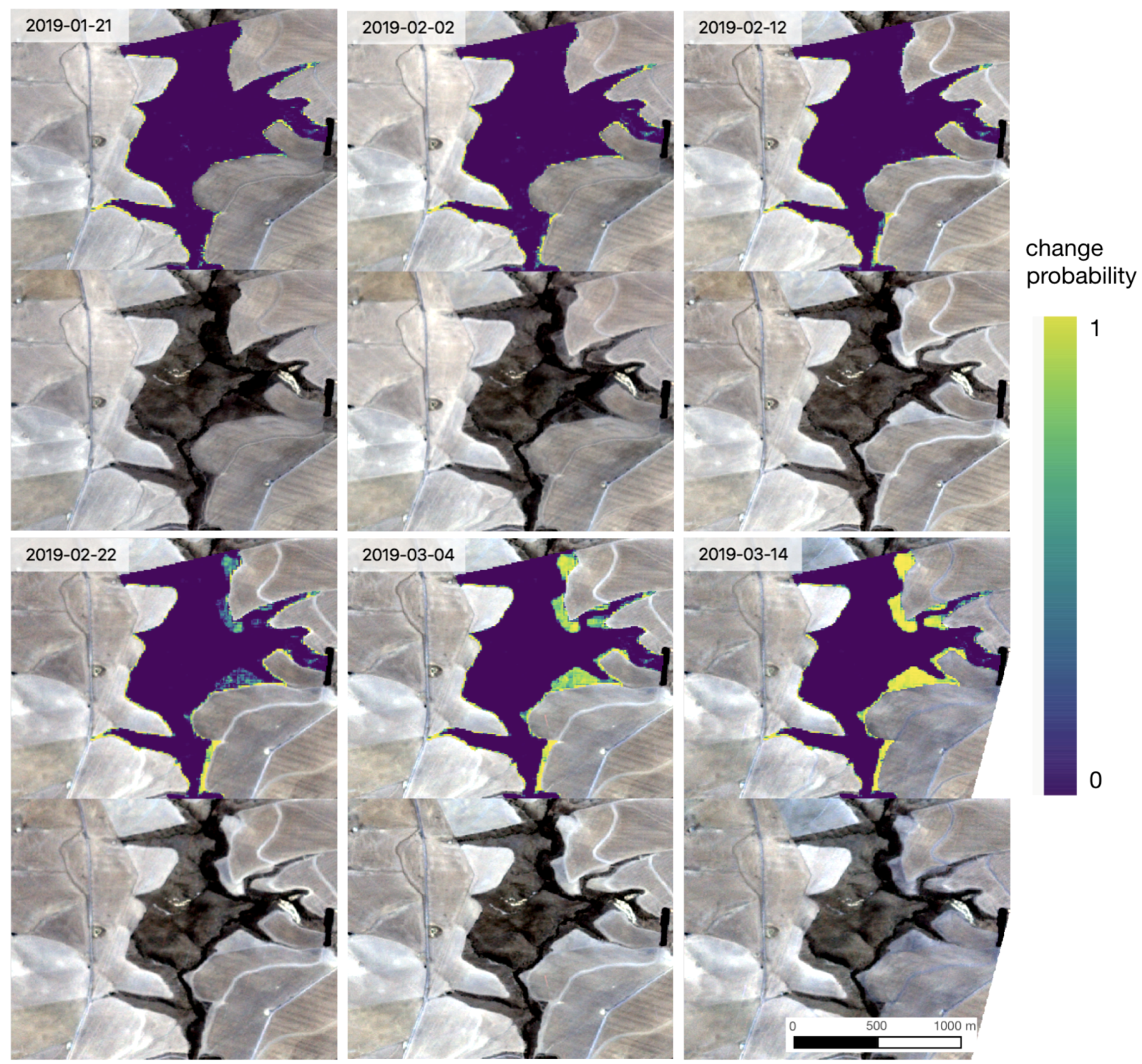
3. Results
4. Discussion
5. Conclusions
Funding
Data Availability Statement
Acknowledgments
Conflicts of Interest
References
- Brondizio, E.S.; Settele, J.; Díaz, S.; Ngo, H.T. Global Assessment Report on Biodiversity and Ecosystem Services of the Intergovernmental Science-Policy Platform on Biodiversity and Ecosystem Services; IPBES: Bonn, Germany, 2019. [Google Scholar]
- Le Roux, J.J.; Hui, C.; Castillo, M.L.; Iriondo, J.M.; Keet, J.H.; Khapugin, A.A.; Médail, F.; Rejmánek, M.; Theron, G.; Yannelli, F.A.; et al. Recent Anthropogenic Plant Extinctions Differ in Biodiversity Hotspots and Coldspots. Curr. Biol. 2019, 29, 2912–2918.e2. [Google Scholar] [CrossRef] [PubMed]
- Turner, W.; Spector, S.; Gardiner, N.; Fladeland, M.; Sterling, E.; Steininger, M. Remote sensing for biodiversity science and conservation. Trends Ecol. Evol. 2003, 18, 306–314. [Google Scholar] [CrossRef]
- Yang, J.; Gong, P.; Fu, R.; Zhang, M.; Chen, J.; Liang, S.; Xu, B.; Shi, J.; Dickinson, R. The role of satellite remote sensing in climate change studies. Nat. Clim. Chang. 2013, 3, 875–883. [Google Scholar] [CrossRef]
- Turner, W. Sensing biodiversity. Science 2014, 346, 301–302. [Google Scholar] [CrossRef]
- Tang, X.; Bullock, E.L.; Olofsson, P.; Estel, S.; Woodcock, C.E. Near real-time monitoring of tropical forest disturbance: New algorithms and assessment framework. Remote Sens. Environ. 2019, 224, 202–218. [Google Scholar] [CrossRef]
- Moffette, F.; Alix-Garcia, J.; Shea, K.; Pickens, A.H. The impact of near-real-time deforestation alerts across the tropics. Nat. Clim. Chang. 2021, 11, 172–178. [Google Scholar] [CrossRef]
- Bond, W.J. Open Ecosystems: Ecology and Evolution beyond the Forest Edge; Oxford University Press: Oxford, UK, 2019. [Google Scholar]
- Poulter, B.; Frank, D.; Ciais, P.; Myneni, R.B.; Andela, N.; Bi, J.; Broquet, G.; Canadell, J.G.; Chevallier, F.; Liu, Y.Y.; et al. Contribution of semi-arid ecosystems to interannual variability of the global carbon cycle. Nature 2014, 509, 600–603. [Google Scholar] [CrossRef] [Green Version]
- Slingsby, J.A.; Moncrieff, G.R.; Wilson, A.M. Near-real time forecasting and change detection for an open ecosystem with complex natural dynamics. ISPRS J. Photogramm. Remote Sens. 2020, 166, 15–25. [Google Scholar] [CrossRef]
- Wilson, A.M.; Latimer, A.M.; Silander, J.A.J. Climatic controls on ecosystem resilience: Postfire regeneration in the Cape Floristic Region of South Africa. Proc. Natl. Acad. Sci. USA 2015, 112, 9058–9063. [Google Scholar] [CrossRef] [Green Version]
- Myers, N.; Mittermeier, R.A.; Mittermeier, C.G.; da Fonseca, G.A.B.; Kent, J. Biodiversity hotspots for conservation priorities. Nature 2000, 403, 853–858. [Google Scholar] [CrossRef]
- Manning, J.; Goldblatt, P. Plants of the Greater Cape Floristic Region. 1: The Core Cape Flora; South African National Biodiversity Institute: Pretoria, South Africa, 2012. [Google Scholar]
- Skowno, A.J.; Poole, C.J.; Raimondo, D.C. National Biodiversity Assessment 2018: The Status of South Africa’s Ecosystems and Biodiversity. Synthesis Report; South African National Biodiversity Institute: Pretoria, South Africa, 2019. [Google Scholar]
- Skowno, A.L.; Jewitt, D.; Slingsby, J.A. Rates and patterns of habitat loss across South Africa’s vegetation biomes. S. Afr. J. Sci. 2021, 117. [Google Scholar] [CrossRef]
- Humphreys, A.M.; Govaerts, R.; Ficinski, S.Z.; Lughadha, E.N.; Vorontsova, M.S. Global dataset shows geography and life form predict modern plant extinction and rediscovery. Nat. Ecol. Evol. 2019, 3, 1043–1047. [Google Scholar] [CrossRef] [PubMed]
- Raimondo, D. The Red List of South African plants: A global first. S. Afr. J. Sci. 2011, 107, 1–2. [Google Scholar] [CrossRef]
- Brummitt, N.A.; Bachman, S.P.; Griffiths-Lee, J.; Lutz, M.; Moat, J.F.; Farjon, A.; Donaldson, J.S.; Hilton-Taylor, C.; Meagher, T.R.; Albuquerque, S.; et al. Green Plants in the Red: A Baseline Global Assessment for the IUCN Sampled Red List Index for Plants. PLoS ONE 2015, 10, e0135152. [Google Scholar] [CrossRef] [PubMed] [Green Version]
- Von Hase, A.; Rouget, M.; Maze, K.; Helme, N. A fine-scale conservation plan for Cape lowlands renosterveld: Technical report. Rep. CCU 2003, 2, 104. [Google Scholar]
- Moncrieff, G.R. Locating and Dating Land Cover Change Events in the Renosterveld, a Critically Endangered Shrubland Ecosystem. Remote Sens. 2021, 13, 834. [Google Scholar] [CrossRef]
- Verbesselt, J.; Zeileis, A.; Herold, M. Near real-time disturbance detection using satellite image time series. Remote Sens. Environ. 2012, 123, 98–108. [Google Scholar] [CrossRef]
- Zhu, Z.; Woodcock, C.E. Continuous change detection and classification of land cover using all available Landsat data. Remote Sens. Environ. 2014, 144, 152–171. [Google Scholar] [CrossRef] [Green Version]
- Ye, S.; Rogan, J.; Zhu, Z.; Eastman, J.R. A near-real-time approach for monitoring forest disturbance using Landsat time series: Stochastic continuous change detection. Remote Sens. Environ. 2021, 252, 112167. [Google Scholar] [CrossRef]
- Zhu, Z.; Zhang, J.; Yang, Z.; Aljaddani, A.H.; Cohen, W.B.; Qiu, S.; Zhou, C. Continuous monitoring of land disturbance based on Landsat time series. Remote Sens. Environ. 2020, 238, 111116. [Google Scholar] [CrossRef]
- Kennedy, R.E.; Townsend, P.A.; Gross, J.E.; Cohen, W.B.; Bolstad, P.; Wang, Y.Q.; Adams, P. Remote sensing change detection tools for natural resource managers: Understanding concepts and tradeoffs in the design of landscape monitoring projects. Remote Sens. Environ. 2009, 113, 1382–1396. [Google Scholar] [CrossRef]
- Hansen, M.C.; Potapov, P.V.; Moore, R.; Hancher, M.; Turubanova, S.A.; Tyukavina, A.; Thau, D.; Stehman, S.V.; Goetz, S.J.; Loveland, T.R. High-resolution global maps of 21st-century forest cover change. Science 2013, 342, 850–853. [Google Scholar] [CrossRef] [PubMed] [Green Version]
- Hansen, M.C.; Krylov, A.; Tyukavina, A.; Potapov, P.V.; Turubanova, S.; Zutta, B.; Ifo, S.; Margono, B.; Stolle, F.; Moore, R. Humid tropical forest disturbance alerts using Landsat data. Environ. Res. Lett. 2016, 11, 034008. [Google Scholar] [CrossRef]
- Kennedy, R.E.; Yang, Z.; Cohen, W.B. Detecting trends in forest disturbance and recovery using yearly Landsat time series: 1. LandTrendr — Temporal segmentation algorithms. Remote Sens. Environ. 2010, 114, 2897–2910. [Google Scholar] [CrossRef]
- Pacheco-Pascagaza, A.M.; Gou, Y.; Louis, V.; Roberts, J.F.; Rodríguez-Veiga, P.; da Conceição Bispo, P.; Espírito-Santo, F.D.B.; Robb, C.; Upton, C.; Galindo, G.; et al. Near Real-Time Change Detection System Using Sentinel-2 and Machine Learning: A Test for Mexican and Colombian Forests. Remote Sens. 2022, 14, 707. [Google Scholar] [CrossRef]
- Wessels, K.J.; Van den Bergh, F.; Roy, D.P.; Salmon, B.P.; Steenkamp, K.C.; MacAlister, B.; Swanepoel, D.; Jewitt, D. Rapid land cover map updates using change detection and robust random forest classifiers. Remote Sens. 2016, 8, 888. [Google Scholar] [CrossRef] [Green Version]
- Habib, T.; Inglada, J.; Mercier, G.; Chanussot, J. Support vector reduction in SVM algorithm for abrupt change detection in remote sensing. IEEE Geosci. Remote Sens. Lett. 2009, 6, 606–610. [Google Scholar] [CrossRef]
- Mas, J.F. Monitoring land-cover changes: A comparison of change detection techniques. Int. J. Remote Sens. 1999, 20, 139–152. [Google Scholar] [CrossRef]
- LeCun, Y.; Bengio, Y.; Hinton, G. Deep learning. Nature 2015, 521, 436–444. [Google Scholar] [CrossRef]
- Ismail Fawaz, H.; Forestier, G.; Weber, J.; Idoumghar, L.; Muller, P.A. Deep learning for time series classification: A review. Data Min. Knowl. Discov. 2019, 33, 917–963. [Google Scholar] [CrossRef] [Green Version]
- Kussul, N.; Lavreniuk, M.; Skakun, S.; Shelestov, A. Deep learning classification of land cover and crop types using remote sensing data. IEEE Geosci. Remote Sens. Lett. 2017, 14, 778–782. [Google Scholar] [CrossRef]
- Rußwurm, M.; Körner, M. Self-attention for raw optical satellite time series classification. arXiv 2019, arXiv:1910.10536. [Google Scholar] [CrossRef]
- Pelletier, C.; Webb, G.I.; Petitjean, F. Temporal Convolutional Neural Network for the Classification of Satellite Image Time Series. Remote Sens. 2019, 11, 523. [Google Scholar] [CrossRef] [Green Version]
- Sefrin, O.; Riese, F.M.; Keller, S. Deep learning for land cover change detection. Remote Sens. 2020, 13, 78. [Google Scholar] [CrossRef]
- Rußwurm, M.; Pelletier, C.; Zollner, M.; Lefèvre, S.; Körner, M. BreizhCrops: A Time Series Dataset for Crop Type Mapping. arXiv 2020, arXiv:1905.11893. [Google Scholar] [CrossRef]
- Zhu, X.X.; Tuia, D.; Mou, L.; Xia, G.S.; Zhang, L.; Xu, F.; Fraundorfer, F. Deep learning in remote sensing: A comprehensive review and list of resources. IEEE Geosci. Remote Sens. Mag. 2017, 5, 8–36. [Google Scholar] [CrossRef] [Green Version]
- Mucina, L.; Rutherford, M.C. (Eds.) The Vegetation of South Africa, Lesotho and Swaziland; Strelitzia 19; South African National Biodiversity Institute: Pretoria, South Africa, 2006. [Google Scholar]
- Douzas, G.; Bacao, F.; Fonseca, J.; Khudinyan, M. Imbalanced Learning in Land Cover Classification: Improving Minority Classes’ Prediction Accuracy Using the Geometric SMOTE Algorithm. Remote Sens. 2019, 11, 3040. [Google Scholar] [CrossRef] [Green Version]
- Johnson, J.M.; Khoshgoftaar, T.M. Survey on deep learning with class imbalance. J. Big Data 2019, 6, 27. [Google Scholar] [CrossRef]
- Simoes, R.; Camara, G.; Queiroz, G.; Souza, F.; Andrade, P.R.; Santos, L.; Carvalho, A.; Ferreira, K. Satellite Image Time Series Analysis for Big Earth Observation Data. Remote Sens. 2021, 13, 2428. [Google Scholar] [CrossRef]
- Vaswani, A.; Shazeer, N.; Parmar, N.; Uszkoreit, J.; Jones, L.; Gomez, A.N.; Kaiser, Ł.; Polosukhin, I. Attention is all you need. In Proceedings of the Annual Conference on Neural Information Processing Systems 2017, Long Beach, CA, USA, 4–9 December 2017; pp. 5998–6008. [Google Scholar]
- Bahdanau, D.; Cho, K.; Bengio, Y. Neural Machine Translation by Jointly Learning to Align and Translate. arXiv 2016, arXiv:1409.0473. [Google Scholar]
- Gorelick, N.; Hancher, M.; Dixon, M.; Ilyushchenko, S.; Thau, D.; Moore, R. Google Earth Engine: Planetary-scale geospatial analysis for everyone. Remote Sens. Environ. 2017, 202, 18–27. [Google Scholar] [CrossRef]
- Chattopadhay, A.; Sarkar, A.; Howlader, P.; Balasubramanian, V.N. Grad-cam++: Generalized gradient-based visual explanations for deep convolutional networks. In Proceedings of the 2018 IEEE winter conference on applications of computer vision (WACV), Lake Tahoe, NV, USA, 12–15 March 2018; pp. 839–847. [Google Scholar]
- Bullock, E.L.; Woodcock, C.E.; Holden, C.E. Improved change monitoring using an ensemble of time series algorithms. Remote Sens. Environ. 2020, 238, 111165. [Google Scholar] [CrossRef]
- Zhou, Q.; Rover, J.; Brown, J.; Worstell, B.; Howard, D.; Wu, Z.; Gallant, A.L.; Rundquist, B.; Burke, M. Monitoring Landscape Dynamics in Central U.S. Grasslands with Harmonized Landsat-8 and Sentinel-2 Time Series Data. Remote Sens. 2019, 11, 328. [Google Scholar] [CrossRef] [Green Version]
- Ye, S.; Rogan, J.; Zhu, Z.; Hawbaker, T.J.; Hart, S.J.; Andrus, R.A.; Meddens, A.J.H.; Hicke, J.A.; Eastman, J.R.; Kulakowski, D. Detecting subtle change from dense Landsat time series: Case studies of mountain pine beetle and spruce beetle disturbance. Remote Sens. Environ. 2021, 263, 112560. [Google Scholar] [CrossRef]
- Parr, C.L.; Lehmann, C.E.; Bond, W.J.; Hoffmann, W.A.; Andersen, A.N. Tropical grassy biomes: Misunderstood, neglected, and under threat. Trends Ecol. Evol. 2014, 29, 205–213. [Google Scholar] [CrossRef]
- Rußwurm, M.; Wang, S.; Korner, M.; Lobell, D. Meta-learning for few-shot land cover classification. In Proceedings of the IEEE/CVF Conference on Computer Vision and Pattern Recognition Workshops, Seattle, WA, USA, 14–19 June 2020; pp. 200–201. [Google Scholar]
- Sun, X.; Wang, B.; Wang, Z.; Li, H.; Li, H.; Fu, K. Research progress on few-shot learning for remote sensing image interpretation. IEEE J. Sel. Top. Appl. Earth Obs. Remote Sens. 2021, 14, 2387–2402. [Google Scholar] [CrossRef]
- Vanschoren, J. Meta-learning. In Automated Machine Learning; Springer: Cham, Switzerland, 2019; pp. 35–61. [Google Scholar]
- Finn, C.; Abbeel, P.; Levine, S. Model-agnostic meta-learning for fast adaptation of deep networks. In Proceedings of the International Conference on Machine Learning, Sydney, Australia, 6–11 August 2017; pp. 1126–1135. [Google Scholar]
- Maus, V.; Câmara, G.; Cartaxo, R.; Sanchez, A.; Ramos, F.M.; De Queiroz, G.R. A time-weighted dynamic time warping method for land-use and land-cover mapping. IEEE J. Sel. Top. Appl. Earth Obs. Remote Sens. 2016, 9, 3729–3739. [Google Scholar] [CrossRef]
- Dempster, A.; Petitjean, F.; Webb, G.I. ROCKET: Exceptionally fast and accurate time series classification using random convolutional kernels. Data Min. Knowl. Discov. 2020, 34, 1454–1495. [Google Scholar] [CrossRef]


| Accuracy | F1 | Recall-1 | Recall-0 | Precision-1 | Precision-0 | Recall-1-Short | |
|---|---|---|---|---|---|---|---|
| Random Forest | 0.98 | 0.88 | 0.79 | 0.99 | 0.98 | 0.98 | 0.50 |
| TempCNN | 0.99 | 0.93 | 0.89 | 0.99 | 0.96 | 0.99 | 0.64 |
| Transformer | 0.99 | 0.92 | 0.88 | 0.99 | 0.97 | 0.99 | 0.60 |
| CCDC | 0.90 | 0.52 | 0.49 | 0.95 | 0.54 | 0.94 | - |
Publisher’s Note: MDPI stays neutral with regard to jurisdictional claims in published maps and institutional affiliations. |
© 2022 by the author. Licensee MDPI, Basel, Switzerland. This article is an open access article distributed under the terms and conditions of the Creative Commons Attribution (CC BY) license (https://creativecommons.org/licenses/by/4.0/).
Share and Cite
Moncrieff, G.R. Continuous Land Cover Change Detection in a Critically Endangered Shrubland Ecosystem Using Neural Networks. Remote Sens. 2022, 14, 2766. https://doi.org/10.3390/rs14122766
Moncrieff GR. Continuous Land Cover Change Detection in a Critically Endangered Shrubland Ecosystem Using Neural Networks. Remote Sensing. 2022; 14(12):2766. https://doi.org/10.3390/rs14122766
Chicago/Turabian StyleMoncrieff, Glenn R. 2022. "Continuous Land Cover Change Detection in a Critically Endangered Shrubland Ecosystem Using Neural Networks" Remote Sensing 14, no. 12: 2766. https://doi.org/10.3390/rs14122766
APA StyleMoncrieff, G. R. (2022). Continuous Land Cover Change Detection in a Critically Endangered Shrubland Ecosystem Using Neural Networks. Remote Sensing, 14(12), 2766. https://doi.org/10.3390/rs14122766