
Using Remote Sensing to Estimate Understorey Biomass in Semi-Arid Woodlands of South-Eastern Australia


Abstract
:
1. Introduction
2. Materials and Methods
2.1. Study Area
2.2. Field Data
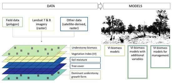
2.3. Satellite Data
2.4. Analysis and Modelling
2.5. Model Validation
3. Results
3.1. Understorey Biomass
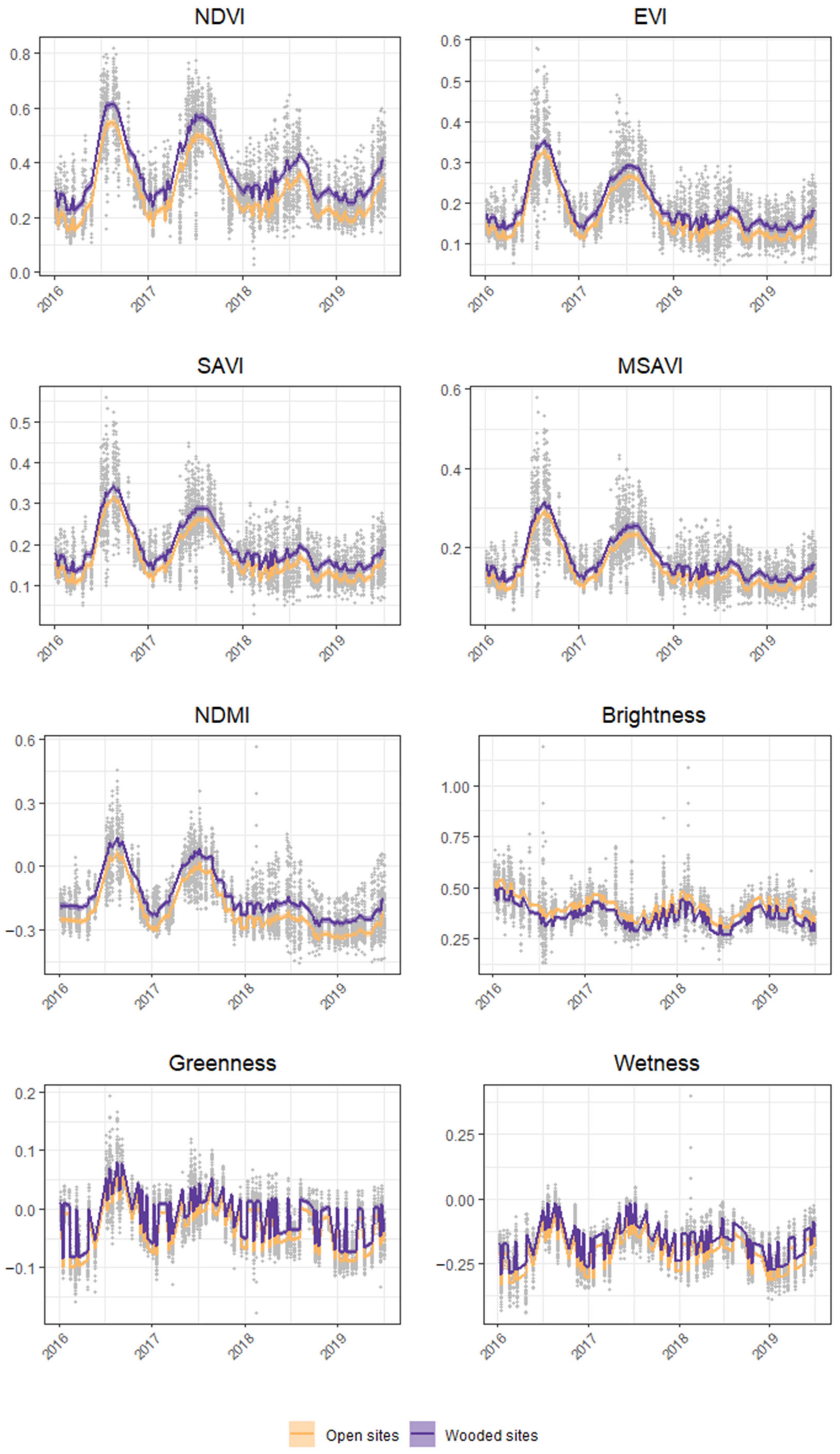
3.2. Vegetation Indices
3.3. Vegetation Index-Biomass Models
3.4. Vegetation Index-Biomass Models with Additional Variables
3.5. Vegetation Index-Biomass Models for Management
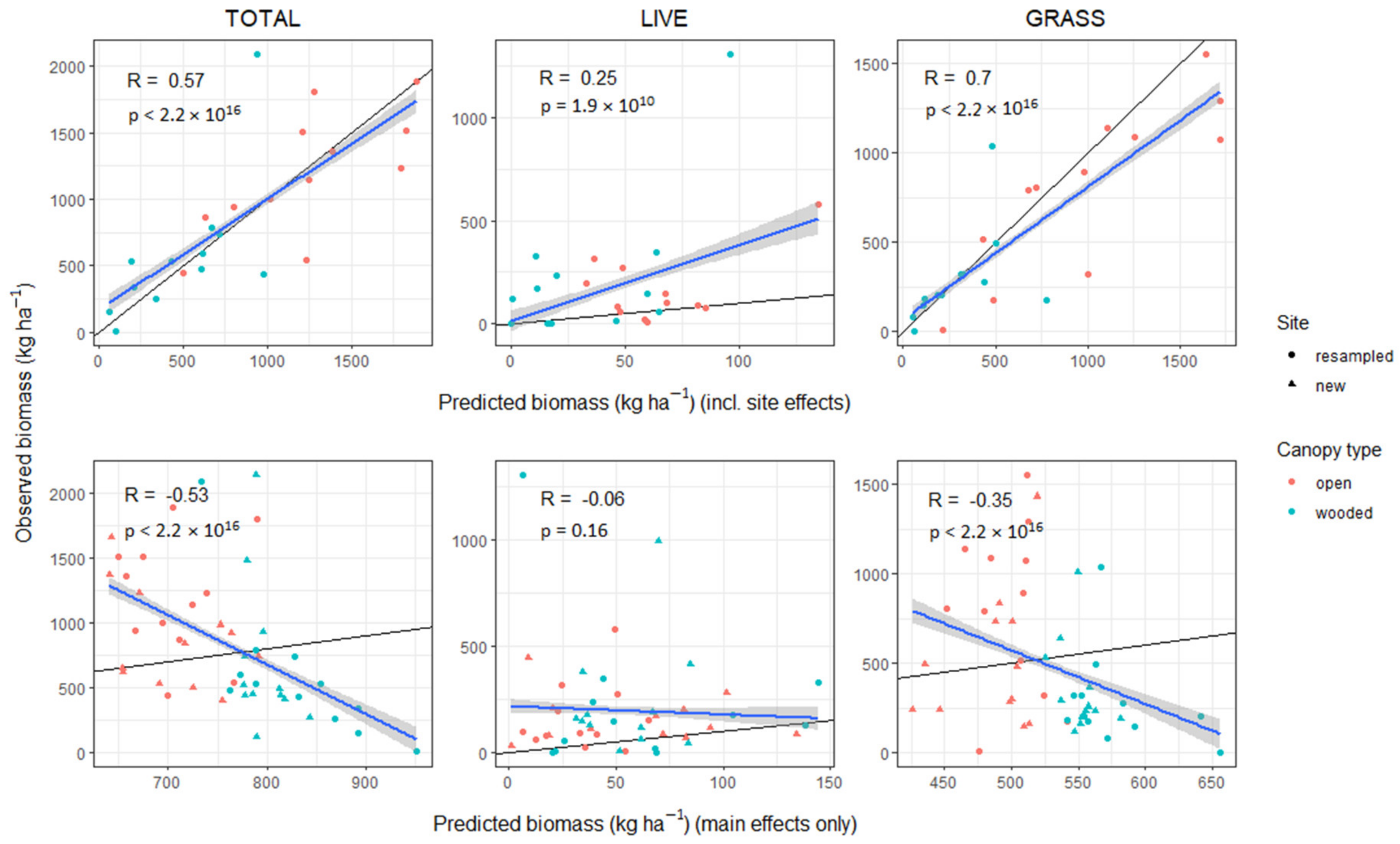
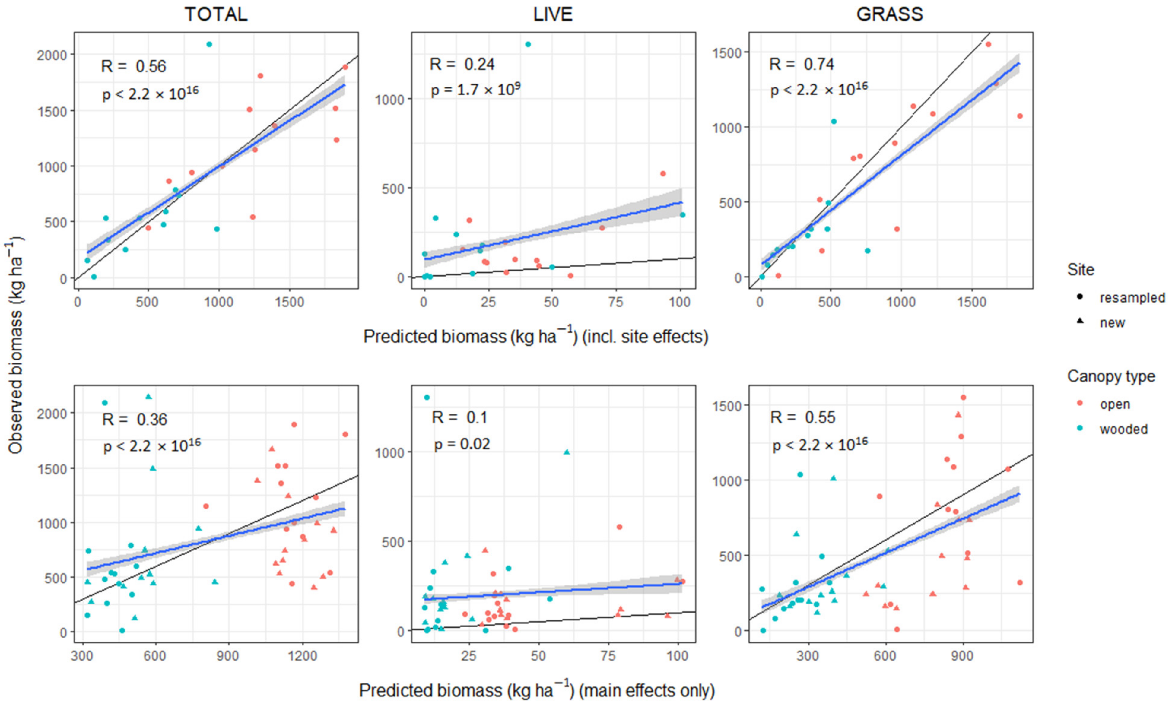
3.6. Model Validation
4. Discussion
4.1. Vegetation Index-Biomass Models
4.2. Vegetation Index-Biomass Models with Additional Variables
4.3. Vegetation Index-Biomass Models for Management
5. Conclusions
Supplementary Materials
Author Contributions
Funding
Data Availability Statement
Acknowledgments
Conflicts of Interest
References
- Keane, R.E.; Burgan, R.; van Wagtendonk, J. Mapping Wildland Fuels for Fire Management across Multiple Scales: Integrating Remote Sensing, GIS, and Biophysical Modeling. Int. J. Wildland Fire 2001, 10, 301–309. [Google Scholar] [CrossRef]
- Kerr, J.T.; Ostrovsky, M. From Space to Species: Ecological Applications for Remote Sensing. Trends Ecol. Evol. 2003, 18, 299–305. [Google Scholar] [CrossRef]
- Wingate, V.R.; Phinn, S.R.; Kuhn, N.; Scarth, P. Estimating Aboveground Woody Biomass Change in Kalahari Woodland: Combining Field, Radar, and Optical Data Sets. Int. J. Remote Sens. 2018, 39, 577–606. [Google Scholar] [CrossRef] [Green Version]
- Ballesteros, R.; Ortega, J.F.; Hernandez, D.; del Campo, A.; Moreno, M.A. Combined Use of Agro-Climatic and Very High-Resolution Remote Sensing Information for Crop Monitoring. Int. J. Appl. Earth Obs. Geoinf. 2018, 72, 66–75. [Google Scholar] [CrossRef]
- Flombaum, P.; Sala, O.E. A Non-Destructive and Rapid Method to Estimate Biomass and Aboveground Net Primary Production in Arid Environments. J. Arid Environ. 2007, 69, 352–358. [Google Scholar] [CrossRef]
- Michez, A.; Lejeune, P.; Bauwens, S.; Herinaina, A.; Blaise, Y.; Castro Muñoz, E.; Lebeau, F.; Bindelle, J. Mapping and Monitoring of Biomass and Grazing in Pasture with an Unmanned Aerial System. Remote Sens. 2019, 11, 473. [Google Scholar] [CrossRef] [Green Version]
- Sinde-González, I.; Gil-Docampo, M.; Arza-García, M.; Grefa-Sánchez, J.; Yánez-Simba, D.; Pérez-Guerrero, P.; Abril-Porras, V. Biomass Estimation of Pasture Plots with Multitemporal UAV-Based Photogrammetric Surveys. Int. J. Appl. Earth Obs. Geoinf. 2021, 101, 102355. [Google Scholar] [CrossRef]
- Walton, K.M.; Spalinger, D.E.; Harris, N.R.; Collins, W.B.; Willacker, J.J. High Spatial Resolution Vegetation Mapping for Assessment of Wildlife Habitat: Mapping for Assessment of Wildlife Habitat. Wildl. Soc. Bull. 2013, 37, 906–915. [Google Scholar] [CrossRef]
- Garroutte, E.; Hansen, A.; Lawrence, R. Using NDVI and EVI to Map Spatiotemporal Variation in the Biomass and Quality of Forage for Migratory Elk in the Greater Yellowstone Ecosystem. Remote Sens. 2016, 8, 404. [Google Scholar] [CrossRef] [Green Version]
- Palmer, A.R.; Samuels, I.; Cupido, C.; Finca, A.; Kangombe, W.F.; Yunusa, I.A.; Vetter, S.; Mapaure, I. Aboveground Biomass Production of a Semi-Arid Southern African Savanna: Towards a New Model. Afr. J. Range Forage Sci. 2016, 33, 43–51. [Google Scholar] [CrossRef]
- Doan, T.; Guo, X. Understanding Bison Carrying Capacity Estimation in Northern Great Plains Using Remote Sensing and GIS. Can. J. Remote Sens. 2019, 45, 139–162. [Google Scholar] [CrossRef]
- Raab, C.; Riesch, F.; Tonn, B.; Barrett, B.; Meißner, M.; Balkenhol, N.; Isselstein, J. Target-oriented Habitat and Wildlife Management: Estimating Forage Quantity and Quality of Semi-natural Grasslands with Sentinel-1 and Sentinel-2 Data. Remote Sens. Ecol. Conserv. 2020, 6, 381–398. [Google Scholar] [CrossRef]
- Baret, F.; Guyot, G.; Major, D.J. TSAVI: A Vegetation Index Which Minimizes Soil Brightness Effects On LAI And APAR Estimation. In Proceedings of the 12th Canadian Symposium on Remote Sensing Geoscience and Remote Sensing Symposium, Vancouver, BC, Canada, 10–14 July 1989; IEEE: Vancouver, Canada, 1989; Volume 3, pp. 1355–1358. [Google Scholar]
- Bannari, A.; Morin, D.; Bonn, F.; Huete, A.R. A Review of Vegetation Indices. Remote Sens. Rev. 1995, 13, 95–120. [Google Scholar] [CrossRef]
- Hardisky, M.A.; Klemas, V.; Smart, R.M. The Influence of Soil Salinity, Growth Form, and Leaf Moisture on the Spectral Radiance of Spartina Alterniflora Canopies. Photogramm. Eng. Remote Sens. 1983, 49, 77–83. [Google Scholar]
- Huete, A.R.; Liu, H.Q.; Batchily, K.; van Leeuwen, W. A Comparison of Vegetation Indices over a Global Set of TM Images for EOS-MODIS. Remote Sens. Environ. 1997, 59, 440–451. [Google Scholar] [CrossRef]
- Rouse, J.W.; Haas, R.H.; Schell, J.A.; Deering, D.W.; Harlan, J.C. Monitoring the Vernal Advancement and Retrogradation (Greenwave Effect) of Natural Vegetation; Texas A&M University Remote Sensing Center: College Station, TX, USA, 1974. [Google Scholar]
- Eisfelder, C.; Kuenzer, C.; Dech, S. Derivation of Biomass Information for Semi-Arid Areas Using Remote-Sensing Data. Int. J. Remote Sens. 2012, 33, 2937–2984. [Google Scholar] [CrossRef]
- Foody, G.M.; Boyd, D.S.; Cutler, M.E.J. Predictive Relations of Tropical Forest Biomass from Landsat TM Data and Their Transferability between Regions. Remote Sens. Environ. 2003, 85, 463–474. [Google Scholar] [CrossRef]
- Samimi, C.; Kraus, T. Biomass Estimation Using Landsat-TM and -ETM+. Towards a Regional Model for Southern Africa? GeoJournal 2004, 59, 177–187. [Google Scholar] [CrossRef]
- Wessels, K.J.; Prince, S.D.; Zambatis, N.; MacFadyen, S.; Frost, P.E.; Van Zyl, D. Relationship between Herbaceous Biomass and 1-km2 Advanced Very High Resolution Radiometer (AVHRR) NDVI in Kruger National Park, South Africa. Int. J. Remote Sens. 2006, 27, 951–973. [Google Scholar] [CrossRef]
- Cho, M.A.; Skidmore, A.K. Hyperspectral Predictors for Monitoring Biomass Production in Mediterranean Mountain Grasslands: Majella National Park, Italy. Int. J. Remote Sens. 2009, 30, 499–515. [Google Scholar] [CrossRef]
- Huete, A.R. A Soil-Adjusted Vegetation Index (SAVI). Remote Sens. Environ. 1988, 25, 295–309. [Google Scholar] [CrossRef]
- Lewis, M. Spectral Characterization of Australian Arid Zone Plants. Can. J. Remote Sens. 2002, 28, 219–230. [Google Scholar] [CrossRef]
- Kaufman, Y.J.; Tanre, D. Atmospherically Resistant Vegetation Index (ARVI) for EOS-MODIS. IEEE Trans. Geosci. Remote Sens. 1992, 30, 261–270. [Google Scholar] [CrossRef]
- Silleos, N.G.; Alexandridis, T.K.; Gitas, I.Z.; Perakis, K. Vegetation Indices: Advances Made in Biomass Estimation and Vegetation Monitoring in the Last 30 Years. Geocarto Int. 2006, 21, 21–28. [Google Scholar] [CrossRef]
- Huete, A.; Didan, K.; Miura, T.; Rodriguez, E.P.; Gao, X.; Ferreira, L.G. Overview of the Radiometric and Biophysical Performance of the MODIS Vegetation Indices. Remote Sens. Environ. 2002, 83, 195–213. [Google Scholar] [CrossRef]
- Chen, Y.; Gillieson, D. Evaluation of Landsat TM Vegetation Indices for Estimating Vegetation Cover on Semi-Arid Rangelands: A Case Study from Australia. Can. J. Remote Sens. 2009, 35, 435–446. [Google Scholar] [CrossRef]
- Qi, J.; Kerr, Y.; Chehbouni, A. External Factor Consideration in Vegetation Index Development. In Proceedings of the CNES, Proceedings of 6th International Symposium on Physical Measurements and Signatures in Remote Sensing, Val D’Isere, France, 17–22 January 1994. [Google Scholar]
- Kauth, R.J.; Thomas, G.S. The Tasselled Cap—A Graphic Description of the Spectral-Temporal Development of Agricultural Crops as Seen by LANDSAT. In Proceedings of the Symposium on Machine Processing of Remotely Sensed Data; Purdue University: West Lafayette, IN, USA, 1976; p. 13. [Google Scholar]
- Huete, A.R.; Jackson, R.D.; Post, D.F. Spectral Response of a Plant Canopy with Different Soil Backgrounds. Remote Sens. Environ. 1985, 17, 37–53. [Google Scholar] [CrossRef]
- Qi, J.; Marsett, R.C.; Heilman, P. Rangeland Vegetation Cover Estimation from Remotely Sensed Data. In Proceedings of the 2nd International Conference on Geospatial Information in Agriculture and Forestry, Lake Buena Vista, FL, USA, 10–12 January 2000. [Google Scholar]
- Jacques, D.C.; Kergoat, L.; Hiernaux, P.; Mougin, E.; Defourny, P. Monitoring Dry Vegetation Masses in Semi-Arid Areas with MODIS SWIR Bands. Remote Sens. Environ. 2014, 153, 40–49. [Google Scholar] [CrossRef]
- Cheal, D. A Park with a Kangaroo Problem. Oryx 1986, 20, 95–99. [Google Scholar] [CrossRef] [Green Version]
- Taylor, L.; Pegler, P. Total Grazing Management Plan for the Restoration of Semi-Arid Woodland and Floodplain Vegetation Communities in North-Western (Mallee) Parks 2016-2021; State Government of Victoria: Melbourne, VIC, Australia, 2016. [Google Scholar]
- Norbury, G.L. Diet Selection and Demography of the Western Grey Kangaroo: Macropus Fuliginosus Melanops Desmarest in Hattah-Kulkyne National Park, Victoria. Ph.D. Thesis, Monash University, Clayton, VIC, Australia, 1987. [Google Scholar]
- Riquelme, L.; Rumpff, L.; Duncan, D.H.; Vesk, P.A. Understanding the Spatiotemporal Dynamics of Understorey Biomass in Semi-Arid Woodlands of South-Eastern Australia. Rangel. J. 2022, 44, 47–59. [Google Scholar] [CrossRef]
- Bureau of Meteorology Monthly Rainfall–076065–Bureau of Meteorology. Available online: http://www.bom.gov.au/jsp/ncc/cdio/weatherData/av?p_nccObsCode=139&p_display_type=dataFile&p_startYear=&p_c=&p_stn_num=076065 (accessed on 27 March 2022).
- Miller, J.; Gibson, M.; Westbrooke, M.; Wilcock, P.; Brown, G. Condition of Vegetation in the Riverine Woodlands of Wyperfeld National Park; Centre for Environmental Management, University of Ballarat: Ballarat, VIC, Australia, 1998. [Google Scholar]
- Reinke, K.; Jones, S. Integrating Vegetation Field Surveys with Remotely Sensed Data. Ecol. Manag. Restor. 2006, 7, S18–S23. [Google Scholar] [CrossRef]
- ’t Mannetje, L.; Haydock, K.P. The Dry-Weight-Rank Method for the Botanical Analysis of Pasture. Grass Forage Sci. 1963, 18, 268–275. [Google Scholar] [CrossRef]
- Riquelme, L.; Rumpff, L.; Duncan, D.H.; Vesk, P.A. OSF|Biom_data.csv. Available online: https://osf.io/4kg6d/ (accessed on 25 November 2021).
- United States Geological Survey ESPA—LSRD. Available online: https://espa.cr.usgs.gov/ (accessed on 27 March 2022).
- Baig, M.H.A.; Zhang, L.; Shuai, T.; Tong, Q. Derivation of a Tasselled Cap Transformation Based on Landsat 8 At-Satellite Reflectance. Remote Sens. Lett. 2014, 5, 423–431. [Google Scholar] [CrossRef]
- Flood, N. Continuity of Reflectance Data between Landsat-7 ETM+ and Landsat-8 OLI, for Both Top-of-Atmosphere and Surface Reflectance: A Study in the Australian Landscape. Remote Sens. 2014, 6, 7952–7970. [Google Scholar] [CrossRef] [Green Version]
- Hastie, T.; Tibshirani, R. Generalized Additive Models. Stat. Sci. 1986, 1, 297–318. [Google Scholar] [CrossRef]
- Wood, S.N. Fast Stable Restricted Maximum Likelihood and Marginal Likelihood Estimation of Semiparametric Generalized Linear Models: Estimation of Semiparametric Generalized Linear Models. J. R. Stat. Soc. Ser. B 2011, 73, 3–36. [Google Scholar] [CrossRef] [Green Version]
- R Core Team. R: A Language and Environment for Statistical Computing; R Foundation for Statistical Computing: Vienna, Austria, 2020. [Google Scholar]
- White, M.; Griffioen, P.; Newell, G. Multi-Temporal Land Cover and Native Vegetation Extent for Victoria; Technical Report No. 311; Department of Environment, Land, Water and Planning, Arthur Rylah Institute for Environmental Research: Heidelberg, VIC, Australia, 2020; p. 29. [Google Scholar]
- Leutner, B.; Horning, N.; Schwalb-Willman, J. RStoolbox: Tools for Remote Sensing Data Analysis. R package version 0.2.6. 2019. Available online: https://CRAN.R-project.org/package=RStoolbox (accessed on 25 November 2021).
- Asuero, A.G.; Sayago, A.; González, A.G. The Correlation Coefficient: An Overview. Crit. Rev. Anal. Chem. 2006, 36, 41–59. [Google Scholar] [CrossRef]
- Dormann, C.F.; Elith, J.; Bacher, S.; Buchmann, C.; Carl, G.; Carré, G.; Marquéz, J.R.G.; Gruber, B.; Lafourcade, B.; Leitão, P.J.; et al. Collinearity: A Review of Methods to Deal with It and a Simulation Study Evaluating Their Performance. Ecography 2013, 36, 27–46. [Google Scholar] [CrossRef]
- Bates, D.; Mächler, M.; Bolker, B.; Walker, S. Fitting Linear Mixed-Effects Models Using Lme4. J. Stat. Softw. 2015, 67, 1–48. [Google Scholar] [CrossRef]
- Logan, M. Biostatistical Design and Analysis Using R: A Practical Guide, 1st ed.; Wiley: Hoboken, NJ, USA, 2010; ISBN 9781405190084. [Google Scholar]
- Akaike, H. Information Theory and an Extension of the Maximum Likelihood Principle. In Proceeding of the Second International Symposium on Information Theory, Tsahkadsor, Armenia, 2–8 September 1971; Akademiai Kiado: Budapest, Hungary, 1973; pp. 267–281. [Google Scholar]
- Burnham, K.P.; Anderson, D.R. Model Selection and Multimodel Inference: A Practical Information-Theoretic Approach, 2nd ed.; Springer-Verlag: New York, NY, USA, 2002; ISBN 9780387953649. [Google Scholar]
- Nakagawa, S.; Schielzeth, H. A General and Simple Method for Obtaining R2 from Generalized Linear Mixed-Effects Models. Methods Ecol. Evol. 2013, 4, 133–142. [Google Scholar] [CrossRef]
- Bureau of Meteorology Australian Landscape Water Balance. Available online: http://www.bom.gov.au/water/landscape/#/sm/Actual/day/ (accessed on 5 February 2020).
- Diouf, A.; Lambin, E.F. Monitoring Land-Cover Changes in Semi-Arid Regions: Remote Sensing Data and Field Observations in the Ferlo, Senegal. J. Arid Environ. 2001, 48, 129–148. [Google Scholar] [CrossRef]
- Nano, C.E.M.; Pavey, C.R. Refining the ‘Pulse-Reserve’ Model for Arid Central Australia: Seasonal Rainfall, Soil Moisture and Plant Productivity in Sand Ridge and Stony Plain Habitats of the Simpson Desert. Austral Ecol. 2013, 38, 741–753. [Google Scholar] [CrossRef]
- Ustin, S.L.; Gamon, J.A. Remote Sensing of Plant Functional Types. New Phytol. 2010, 186, 795–816. [Google Scholar] [CrossRef]
- Wehlage, D.; Gamon, J.; Thayer, D.; Hildebrand, D. Interannual Variability in Dry Mixed-Grass Prairie Yield: A Comparison of MODIS, SPOT, and Field Measurements. Remote Sens. 2016, 8, 872. [Google Scholar] [CrossRef] [Green Version]
- Mbow, C.; Fensholt, R.; Rasmussen, K.; Diop, D. Can Vegetation Productivity Be Derived from Greenness in a Semi-Arid Environment? Evidence from Ground-Based Measurements. J. Arid Environ. 2013, 97, 56–65. [Google Scholar] [CrossRef]
- Huete, A.; Justice, C.; Liu, H. Development of Vegetation and Soil Indices for MODIS-EOS. Remote Sens. Environ. 1994, 49, 224–234. [Google Scholar] [CrossRef]
- Tongway, D.J.; Ludwig, J.A. Small-Scale Resource Heterogeneity in Semi-Arid Landscapes. Pac. Conserv. Biol. 1994, 1, 201–208. [Google Scholar] [CrossRef]
- Graetz, R.D. Satellite Remote Sensing of Australian Rangelands. Remote Sens. Environ. 1987, 23, 313–331. [Google Scholar] [CrossRef]
- Moleele, N.; Ringrose, S.; Arnberg, W.; Lunden, B.; Vanderpost, C. Assessment of Vegetation Indexes Useful for Browse (Forage) Prediction in Semi-Arid Rangelands. Int. J. Remote Sens. 2001, 22, 741–756. [Google Scholar] [CrossRef]
- Vermote, E.; Justice, C.; Claverie, M.; Franch, B. Preliminary Analysis of the Performance of the Landsat 8/OLI Land Surface Reflectance Product. Remote Sens. Environ. 2016, 185, 46–56. [Google Scholar] [CrossRef]
- Todd, S.W.; Hoffer, R.M.; Milchunas, D.G. Biomass Estimation on Grazed and Ungrazed Rangelands Using Spectral Indices. Int. J. Remote Sens. 1998, 19, 427–438. [Google Scholar] [CrossRef]
- Svoray, T.; Shoshany, M. SAR-Based Estimation of Areal Aboveground Biomass (AAB) of Herbaceous Vegetation in the Semi-Arid Zone: A Modification of the Water-Cloud Model. Int. J. Remote Sens. 2002, 23, 4089–4100. [Google Scholar] [CrossRef]
- Li, A.; Dhakal, S.; Glenn, N.; Spaete, L.; Shinneman, D.; Pilliod, D.; Arkle, R.; McIlroy, S. Lidar Aboveground Vegetation Biomass Estimates in Shrublands: Prediction, Uncertainties and Application to Coarser Scales. Remote Sens. 2017, 9, 903. [Google Scholar] [CrossRef] [Green Version]
- Anderson, K.E.; Glenn, N.F.; Spaete, L.P.; Shinneman, D.J.; Pilliod, D.S.; Arkle, R.S.; McIlroy, S.K.; Derryberry, D.R. Estimating Vegetation Biomass and Cover across Large Plots in Shrub and Grass Dominated Drylands Using Terrestrial Lidar and Machine Learning. Ecol. Indic. 2018, 84, 793–802. [Google Scholar] [CrossRef]


| Vegetation Index | Formula | References |
|---|---|---|
| Normalised Difference Vegetation Index (NDVI) | (NIR−Red)/(NIR + Red) | [17] |
| Enhanced Vegetation Index (EVI) | 2.5 × ((NIR − Red)/(NIR + 6 × Red − 7.5 × Blue + 1)) | [27] |
| Soil Adjusted Vegetation Index (SAVI) | ((NIR − Red)/(NIR + Red + L)) × (1 + 0.5) | [23] |
| Modified Soil Adjusted Vegetation Index (MSAVI) | (2 × NIR + 1 − √ ((2 × NIR + 1)2 – 8 × (NIR - Red)))/2 | [29] |
| Normalised Difference Moisture Index (NDMI) | (NIR − SWIR1)/(NIR + SWIR1) | [15] |
| Tasselled Cap Brightness | 0.3029(Blue) + 0.2786(Green) + 0.4733(Red) + 0.5599(NIR) + 0.508(SWIR1) + 0.1872(SWIR2) | [30,44] |
| Tasselled Cap Greenness | −0.2941(Blue) + −0.243(Green) + −0.5424(Red) + 0.7276(NIR) + 0.0713(SWIR1) + −0.1608(SWIR2) | [30,44] |
| Tasselled Cap Wetness | 0.1511(Blue) + 0.1973(Green) + 0.3283(Red) + 0.3407(NIR) + −0.7117(SWIR1) + −0.4559(SWIR2) | [30,44] |
| Variable | Resolution | Summary |
|---|---|---|
| Soil moisture | 5 km × 5 km; Daily. | Root zone (top 1 m of soil profile) soil moisture obtained from the BoM Australian Landscape Water Balance (AWRA-L model) [58]. A mean soil moisture window of the previous month, with 2-week lag from clipping date, was chosen as it was most influential for understorey biomass in this study area [37]. |
| Tree cover | 22 m × 27 m approx. | Remotely sensed estimates of the probability of native tree cover [49]. |
| Dominant understorey growth form | 90 m × 90 m; Seasonal. | Growth forms were classified into annual graminoids, perennial graminoids, forbs, and shrubs. Dominant growth form was estimated at each site following the dry-weight-rank method [41]. |
| Model | R2m | R2c | t Value of Predictors |
|---|---|---|---|
| TOTAL ~ Greenness + εi | 0.026 | 0.897 | 14.26 |
| LIVE ~ Brightness + MSAVI + εi | 0.441 | 0.715 | 14.16, 35.43 |
| GRASS ~ Brightness + Greenness + εi | 0.016 | 0.878 | −7.64, 3.33 |
| Model | R2m | R2c | t Value of Predictors |
|---|---|---|---|
| TOTAL ~ Greenness + S.M. + Tree C. + Dom. G.F. + εi | 0.428 | 0.881 | 12.78, −0.25, −6.89, 40.07, 38.66, 40.87, 39.61 |
| LIVE ~ EVI + S.M. + Tree C. + Dom. G.F. + εi | 0.602 | 0.746 | 3.34, 25.49, −3.40, 34.17, 33.67, 41.33, 37.15 |
| GRASS ~ Brightness + Greenness + S.M. + Tree C. + Dom. G.F. + εi | 0.483 | 0.890 | −5.49, 5.03, −1.53, −7.01, 35.21, 26.26, 34.16, 29.73 |
| Model | R2m | R2c | t Value of Predictors |
|---|---|---|---|
| TOTAL ~ Greenness + S.M. + Tree C. + εi | 0.321 | 0.870 | 15.33, 0.44, −6.49 |
| LIVE ~ EVI + S.M. + Tree C. + εi | 0.443 | 0.726 | 2.70, 19.73, −1.30 |
| GRASS ~ Brightness + Greenness + S.M. + Tree C. + εi | 0.312 | 0.844 | −4.65, 9.08, −0.16, −6.76 |
Publisher’s Note: MDPI stays neutral with regard to jurisdictional claims in published maps and institutional affiliations. |
© 2022 by the authors. Licensee MDPI, Basel, Switzerland. This article is an open access article distributed under the terms and conditions of the Creative Commons Attribution (CC BY) license (https://creativecommons.org/licenses/by/4.0/).
Share and Cite
Riquelme, L.; Duncan, D.H.; Rumpff, L.; Vesk, P.A. Using Remote Sensing to Estimate Understorey Biomass in Semi-Arid Woodlands of South-Eastern Australia. Remote Sens. 2022, 14, 2358. https://doi.org/10.3390/rs14102358
Riquelme L, Duncan DH, Rumpff L, Vesk PA. Using Remote Sensing to Estimate Understorey Biomass in Semi-Arid Woodlands of South-Eastern Australia. Remote Sensing. 2022; 14(10):2358. https://doi.org/10.3390/rs14102358
Chicago/Turabian StyleRiquelme, Linda, David H. Duncan, Libby Rumpff, and Peter Anton Vesk. 2022. "Using Remote Sensing to Estimate Understorey Biomass in Semi-Arid Woodlands of South-Eastern Australia" Remote Sensing 14, no. 10: 2358. https://doi.org/10.3390/rs14102358
APA StyleRiquelme, L., Duncan, D. H., Rumpff, L., & Vesk, P. A. (2022). Using Remote Sensing to Estimate Understorey Biomass in Semi-Arid Woodlands of South-Eastern Australia. Remote Sensing, 14(10), 2358. https://doi.org/10.3390/rs14102358