Article

Online Sequential Extreme Learning Machine-Based Active Interference Activity Prediction for Cognitive Radar

National Laboratory of Radar Signal Processing, Xidian University, Xi’an 710071, China
*
Author to whom correspondence should be addressed.
Remote Sens. 2022, 14(12), 2737; https://doi.org/10.3390/rs14122737
Submission received: 27 April 2022 / Revised: 31 May 2022 / Accepted: 6 June 2022 / Published: 7 June 2022
(This article belongs to the Special Issue Radar High-Speed Target Detection, Tracking, Imaging and Recognition)

Abstract

:
For anti-active-interference-oriented cognitive radar systems, the mismatch between the acquired and actual interference information may result in serious degradation of cognitive anti-active-interference performance. To yield more effective knowledge of the electromagnetic environment and eliminate the mismatch effect, the electromagnetic activity prediction technique, which deduces future electromagnetic behaviors based on current observations, has received increasing attention. However, high computational complexities limit the application of conventional electromagnetic activity prediction methods in dynamic active interference prediction with high real-time requirements. In this paper, the online sequential extreme learning machine (OS-ELM)-based method, which is dedicated to high-efficiency active interference activity prediction, is proposed. The advancement includes two aspects. First, benefiting from the single-hidden-layer network structure and recursive-formula-based output weight updating, the proposed OS-ELM-based frequency prediction (OS-ELM-FP) and OS-ELM-based angle prediction (OS-ELM-AP) models can predict the interference state and update the prediction model parameters with much higher computational efficiency. Second, the better generalization performance enables the proposed method to achieve smaller interference activity prediction errors compared with conventional methods. Numerical examples and prediction results based on measured jamming data demonstrate the advantages of the proposed method.

Graphical Abstract

1. Introduction

With the rapid development of jammer technology and the increasing demand for wireless services, active interference has seriously deteriorated the working electromagnetic environment of radar and has become a major obstacle to radar functionality. To counter active interference, passive processing technology performed at the radar receiver has been well developed [1,2,3]. It improves the purity of the target echo by identifying and eliminating the active interference in received signals. Such methods usually work for certain interference types and have anti-interference capabilities limited by the degree of freedom (DOF) of the radar receiver. Therefore, an advanced anti-active interference technique has been regarded as a core requirement for modern radar.
The cognitive radar technique, which improves radar performance via environment sensing and transmitted waveform design, has received increasing attention in the radar community due to its excellent effect and considerable application prospects [4,5,6,7,8,9,10]. For countering active interference by cognitive radar systems, the dynamic changes in active interference, and the delays caused by radar processing, will result in a mismatch between the observed interference information and the actual information. With outdated interference information, the cognitive anti-interference method cannot achieve the maximum anti-interference gain. To mitigate this problem, some robust cognitive anti-interference methods have been proposed to reduce the sensitivity of interference suppression to interference sensing errors to maintain the anti-interference performance [11,12]. However, these methods often come at the cost of the interference cancellation ratio and cannot fundamentally solve the mismatch loss problem. Since improving the effectiveness of active interference information can mitigate the mismatch effect and suppress other processing losses while countering active interference, it has become an urgent issue for the anti-interference of cognitive radar.
Activity prediction can deduce future environmental states based on observations to improve the accuracy of environmental knowledge, which has been extensively studied in the communication field [13,14,15], and a few research results have been extended to radar applications [8,9,16,17,18,19,20,21,22]. These prediction methods can be divided into model-based and model-independent methods, and the main techniques involve Markov process-based prediction [8,9,10,16,18], stochastic process-based prediction [19,20] and machine learning-based prediction [21,22]. Stinco et al. [18] presented a single-channel hidden Markov model (HMM)-based prediction method. This method can effectively model dynamic spectrum access but cannot handle a prediction problem with a large state space. In [9,10], the Markov decision process and partially observable Markov decision process were introduced to model dynamic active interference behavior, and the deep Q network was introduced to solve the model and to overcome the large state space problem. However, these methods require considerable amounts of memory storage space and computing time to converge to the optimal solution. In [20], researchers proposed an angle prediction method based on Gaussian process regression (GPR). GPR is a nonparametric regression model driven by training data but the computational complexity of this method increases significantly with increasing training sizes, which makes it difficult for it to handle large datasets or dynamically updated datasets. In addition, GPR-based prediction methods need to properly set the kernel function, mean function and hyperparameter distribution. In contrast, deep learning methods reduce the impact of manually setting parameters and can extract training sample features in a more automatic way. Among these deep learning methods, long short-term memory (LSTM) is a recurrent neural network (RNN) used for modeling stochastic processes that can learn the short-term and long-term dependencies of time series [21,22] to obtain better forecasting results. However, LSTM-based prediction algorithms have high computational complexities and are also not capable of handling dynamic updated datasets with real-time requirements. Moreover, the generalization ability of LSTM cannot be guaranteed in small sample scenarios.
In a noncooperative active interference environment, the obtained effective interference dataset is limited and dynamically updated by the interaction between radar and active interference. To ensure the interference activity prediction performance, it is necessary to update the prediction model online based on the limited new data. In addition, from the perspective of anti-interference, dynamic countermeasure scenarios require real-time anti-interference operations. Therefore, it is of great significance to construct a real-time online updated active interference prediction model. An extreme learning machine (ELM) adopts a single-layer feedforward neural network (SLFN) structure, which includes an input layer, a hidden layer and an output layer [23,24]. The weight and bias between the input and hidden layers are randomized in advance, and only the weight of the output layer is calculated by the l2 loss function in the training phase. Studies have shown that, through such a network structure and training rules, the model has a higher generalization performance and learning speed [25,26]. Based on these advantages, Liang et al. proposed the online sequential-ELM (OS-ELM) incremental learning algorithm [27,28]. This algorithm updates the output weights of the ELM network based on newly obtained data to enhance the original training model to adapt to the dynamic environment.
In this paper, an OS-ELM-based method, which has a high learning speed and strong generalization ability, is proposed for predicting active interference behavior. Specifically, the OS-ELM-based interference frequency prediction (OS-ELM-FP) model and the OS-ELM-based interference angle prediction (OS-ELM-AP) model are proposed for learning interference activity in the frequency and spatial domains, respectively. As the model parameters are updated efficiently, based on dynamically obtained active interference data, the proposed methods effectively predict interference behavior. The research contributions of this paper are summarized as follows:
(1)
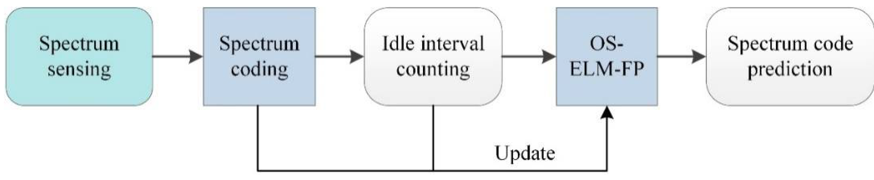
The OS-ELM-FP algorithm is proposed to predict the active interference activity in the frequency domain. Frequency state encoding is first performed on the perceived active interference spectrum to reduce the computational complexity of the prediction. Then, the OS-ELM-FP network architecture is constructed based on the interference state code to predict multichannel interference states in parallel, and the corresponding updating method for the OS-ELM-FP is given. With the single OS-ELM-FP network prediction model, the interference state in multiple frequency channels can be simultaneously predicted efficiently and accurately.
(2)
By constructing the single-input single-output OS-ELM-AP network model and deducing the corresponding updating formula, the OS-ELM-AP algorithm is proposed to predict active interference activity in the spatial domain. Based on the current interference direction estimates, the future interference angle can be efficiently predicted by the proposed method, and the cognitive anti-interference performance in the spatial domain is, thus, improved.
(3)
The prediction performance comparisons of various typical interference frequency schemes (including the two-state Markov process, the triangular sweep mode, the barrage interference and the stochastic interference with a certain probability) are presented in the analysis stage. Both the ballistic simulation data and the measured jamming data are accessed in the analysis stage of the interference state prediction in the spatial domain, which provides a detailed performance analysis of the proposed OS-ELM-AP model.
The rest of the paper is organized as follows. Section 2 presents the anti-interference model for cognitive radar. Section 3 provides the active interference activity prediction method. Section 4 presents the results and corresponding analyses. Finally, the conclusion is drawn in Section 5.

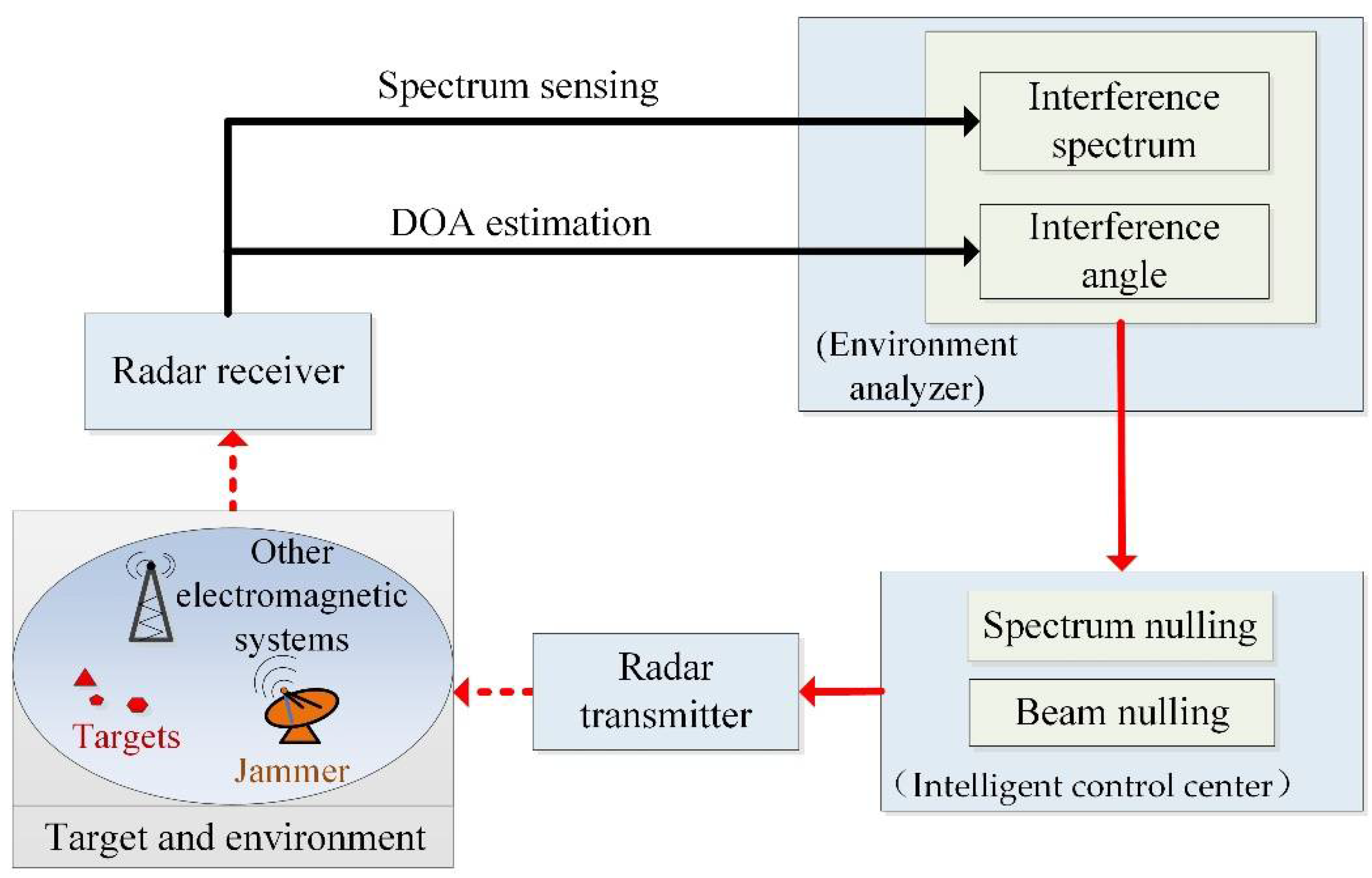
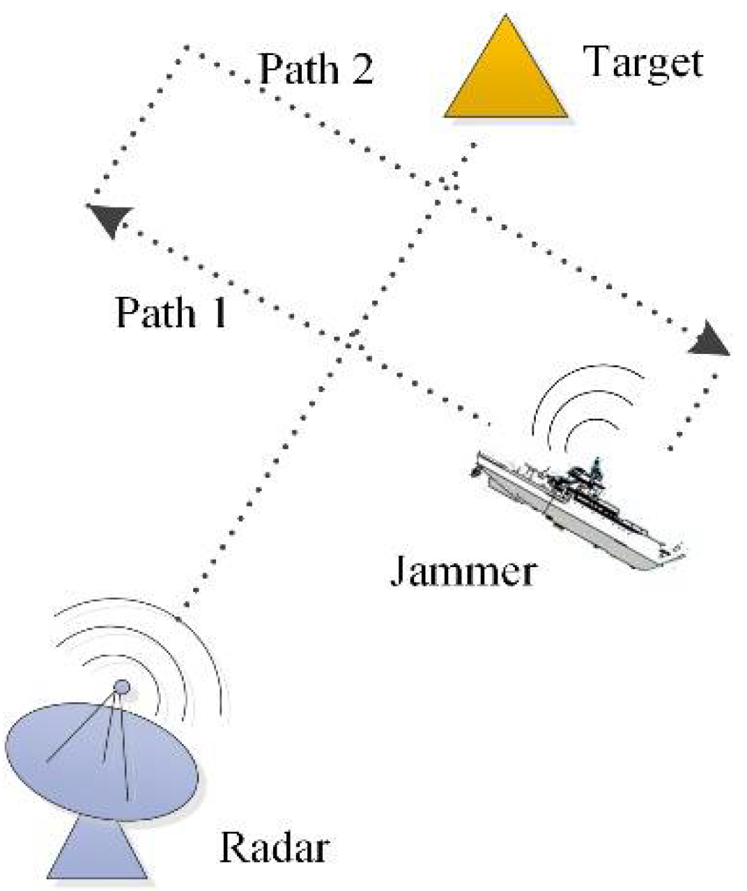
2. Anti-Active Interference Model for Cognitive Radar

We consider cognitive radar with spectrum sensing, direction of arrival (DOA) estimation, target detection and transmit design functions, the anti-interference framework of which is presented in Figure 1. Based on the radar environment analyzer, the perception of active interference can be completed, and the interference spectrum and angle information can be obtained [29,30,31,32]. Based on this information, the intelligent control center designs the transmit waveform to realize the transmit spectrum and beam nulling to avoid co-frequency active interference and reduce the probability of being intercepted by a hostile jammer. According to the transmit waveform provided by the intelligent control center, the radar transmitter transmits a waveform suitable for the environment. Then, the cognitive anti-interference framework is circulated until the target detection performance meets the requirements.
Specifically, consider a uniform linear array with Q elements separated by distance d . The emission steering vector is
a ( θ ) = [ 1 , e j 2 π d λ sin ( θ ) , , e j 2 π ( Q 1 ) d λ sin ( θ ) ]
Assuming that the estimated interference azimuth is θ j , the transmit beam with the notch formed in the interference direction can be synthesized by
ψ : , n = ψ : , n K n a H ( θ j ) , n = 1 , , N p
where ψ is the Q × NP-dimensional transmit matrix, ( ) : , n is the nth column of the matrix, ( ) H is the transpose conjugate operation and K n is the beam amplitude in θ j :
K n = 1 Q q = 1 Q ( ψ : , n a T ( θ j ) ) q , n = 1 , , N p
where ( ) T refers to the transposition operation. Similarly, with the obtained interference frequency f j , the transmit waveform with the notch at f j to avoid active interference can be formed by
ψ q , : = ψ q , : K q e j 2 π f j t , q = 1 , , Q
where ( ) q , : is the qth row of the matrix, t = [ 0 , t s , , t s ( N p 1 ) ] , t s is the sampling interval, and K q  is the amplitude of the transmitted spectrum at fj:
K q = 1 N p n = 1 N p ( ψ q , : e j 2 π f j t ) n , q = 1 , , Q
Equations (2) and (4) give the methods for forming a single notch at the transmit beam and spectrum, respectively, which can easily be extended to the case of forming multiple notches to counter multiple interference, that is,
ψ : , n = ψ : , n K n j 1 a H ( θ j 1 ) K n j η a H ( θ j η ) , n = 1 , , N p
ψ q , : = ψ q , : K q j 1 e j 2 π f j 1 t K q j γ e j 2 π f j γ t , q = 1 , , Q
where η is the number of different directions occupied by active interference, and γ is the number of frequency points occupied by active interference.
Anti-active interference is a perception-reaction process. For the cognitive anti-interference technology designed for the transmitter, as described in (2) and (4), the interference information is sensed, based on the previously received signal. Due to the flexibility of active interference and the time delays caused by the sensing and anti-interference methods, there may be a mismatch between the acquired interference information and the real interference state at the anti-interference moment. In this case, the interference information [ θ j , f j ] is outdated and, hence, greatly reduces the anti-interference performance of cognitive radar.

3. Active Interference Activity Prediction Method

To solve the problem created by outdated active interference knowledge, research on interference behavior prediction was conducted in this section. Based on the observed interference data, the interference state prediction model was constructed to deduce the future interference state to improve the effectiveness of the interference information, thereby maximizing the cognitive radar anti-interference performance.

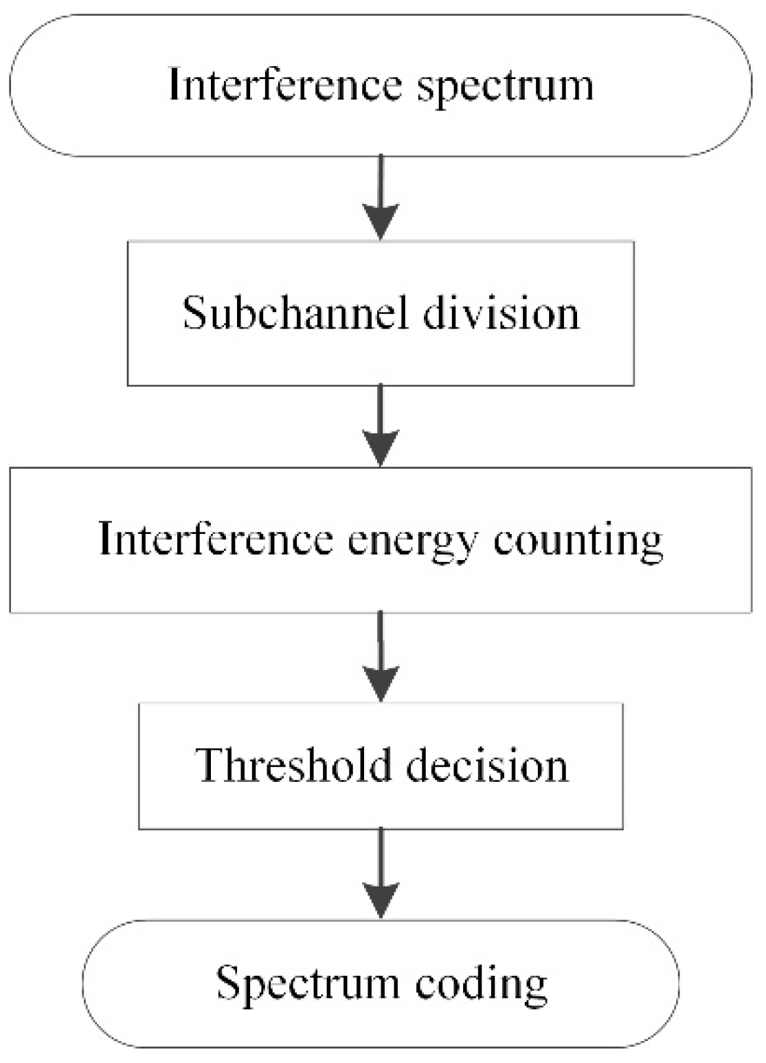
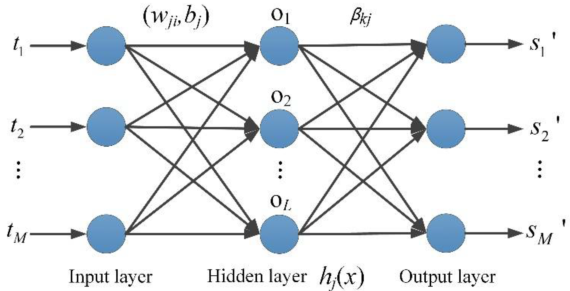
3.1. OS-ELM-FP-Based Active Interference State Prediction in the Frequency Domain

The frequency domain is a major electronic warfare domain. There are many cognitive methods for countering active interference in the frequency domain, such as transmit spectrum nulling and frequency agility. However, the performance of these cognitive anti-interference methods is not stable. The main reason is that the active interference spectrum is flexibly changeable, which leads to a lack of timeliness of the estimated interference frequency information. In this subsection, we propose the OS-ELM-FP method for predicting active interference activity in the frequency domain to obtain effective interference frequency knowledge in real time.
The block diagram of the active interference state prediction in the frequency domain is shown in Figure 2. If the prediction is directly performed on the interference spectrum amplitudes at all frequency points, the computational complexity will be very high. To avoid this, the interference spectrum was first encoded. Then, based on the interference spectrum code, the idle intervals of multiple frequency channels were calculated. Finally, the OS-ELM-FP network model was constructed to predict the interference spectrum code in the next time based on the input idle intervals. In the online prediction stage, the parameters of the OS-ELM-FP network model were updated, based on the dynamically updated interference spectrum and idle interval, to improve the adaptability of the OS-ELM-FP to the dynamically changing active interference environment.
In the spectrum coding stage, the spectrum sensing range of the radar system was divided into multiple subchannels, and a binary vector s was used to represent the active interference spectrum state. When a subchannel was encoded as 0, the active interference in the subchannel was considered negligible, and when the code was 1, the subchannel was considered to be occupied by active interference with sufficient energy. A block diagram of interference spectrum coding is shown in Figure 3. First, the spectrum sensing bandwidth was divided into M frequency subchannels with the minimum working bandwidth of the radar system as an interval. Then, the received interference signal energy in each subchannel was counted, and the channel code was determined based on a threshold decision. If the counted interference energy was less than the decision threshold, the corresponding subchannel was coded as 0, while the subchannel was coded as 1 if the interference energy was greater than the decision threshold.
An example of interference spectrum coding is given in Figure 4. The spectrum sensing bandwidth and the minimum working bandwidth were set to 100 MHz and 20 MHz, respectively, so a total of 5 subchannels were divided. The noise level in the subchannel was counted, based on signals received from angle-range bins without active interference sources. With the obtained noise level, the decision threshold could be determined by using the Neyman-Pearson criterion. Then, the state code s = [ 1   0   0   1   0 ] T could be obtained for the interference spectrum in Figure 4. The coding result indicated that the first and fourth subchannels were occupied by active interference. In addition to the threshold determination method, based on the Neyman-Pearson criterion, the posterior probability of active interference identification, which does not require environmental knowledge, is also suitable for the decision in a noncooperative interference environment. Related details can be obtained by referring to [10].
Based on the interference spectrum code s , the continuous idle interval of each subchannel could be accumulated. Then, the idle interval vector t = [ t 1 , t 2 , , t M ] T could be obtained. Taking t as the input of the OS-ELM-FP network, the interference state binary vector s = [ s 1 , s 2 , , s M ] T at the next moment could be predicted. Therefore, the OS-ELM-FP network model with M-dimensional input and M-dimensional output was constructed, as shown in Figure 5. The weight and bias used to connect the input and hidden layers of the OS-ELM-FP network were expressed as
( w j i , b j ) , j = 1 , , L ; i = 1 , , M
In OS-ELM-FP, the value of ( w , b ) was set randomly, or based on offline training data, and would not be updated during the online test phase. Let h j be the output of the hidden layer. h j was expressed as
h j = g ( w j , : t + b j )
where g ( x ) was the transfer function of the hidden layer of the OS-ELM-FP network. The weight of the output layer of the OS-ELM-FP network was expressed as
β k j , k = 1 , , M ; j = 1 , , L
Hence, the output of the OS-ELM-FP network was defined as
s = β h = β g ( w t + b )
During the training phase, the OS-ELM-FP determined the weight of the output layer by minimizing the squared difference between the prediction results and the sensed interference states. The computing formula was given by
β ^ = s T H
where s T was the frequency state of active interference perceived at the next time, and ( ) was the pseudoinverse operation.
H = [ h 1 , h 2 , , h N ]
where N was the number of offline training samples. In the online test phase, state coding was performed on the newly obtained active interference spectrum, and the idle interval vector t was updated according to the new spectrum code. Then, based on the updated idle interval vector t and interference spectrum code s T , the output weight of the OS-ELM-FP network was updated by
β v + 1 = β v + ( s T v + 1 β v H v + 1 ) H v + 1
where v was the number of updates.
The prediction and updating steps of the OS-ELM-FP network model are summarized in Algorithm 1.
Algorithm 1 OS-ELM-FP-based interference frequency prediction
Perform the following in the offline training phase.
(1) Encode the active interference frequency state based on the radar system settings (spectrum sensing bandwidth and minimum working bandwidth), and count the idle interval vector t based on the state codes.
(2) Determine the OS-ELM-FP network structure according to the dimension of the interference spectrum code, and randomly set the weight and bias connecting the input and hidden layers of the OS-ELM-FP network.
(3) Compute the weight of the output layer by (12).
Perform the following in the online training phase.
(4) Update the idle interval vector t based on the updated interference spectrum code, and update the output weight of the OS-ELM-FP network by (14).

3.2. OS-ELM-AP-Based Active Interference State Prediction in the Spatial Domain

Although the variation in the interference in the spatial domain is not as flexible as that in the frequency domain, a small deviation in the estimated interference direction can greatly degrade the anti-interference performance in the spatial domain. Therefore, an active interference angle prediction method was investigated in this subsection.
The prediction of the active interference state in the spatial domain refers to predicting the interference angle θ at the next moment with the previous estimated interference angle θ . Therefore, the single-input and single-output OS-ELM-AP network was constructed as shown in Figure 6.
The weight and bias used to connect the input and hidden layers of the OS-ELM-AP network were expressed as
( w j s , b j s ) , j = 1 , , L
The output h j s of the hidden layer of the OS-ELM-AP was defined as
h j s = g s ( w j s θ + b j s ) , j = 1 , , L
where g s ( x ) was the transfer function of the hidden layer of the OS-ELM-AP network. The output weight of the OS-ELM-AP network was denoted as β j s , j = 1 , , L . The output of the OS-ELM-AP network was defined as
θ = β s h s = β s g s ( w s θ + b s )
Similarly, the values of the weight and bias used to connect the input and hidden layers of the OS-ELM-AP network were randomly generated in the offline phase. During the online learning phase, the weight and bias were not updated, and only the weight β s between the hidden and output layers was updated, based on the newly obtained interference DOA estimation data. Specifically, in the training phase, the calculation formula of the output weight was
β ^ s = θ T H s
where θ T was the training label, and
H s = [ h 1 s , h 2 s , , h N s ]
In the online testing phase, the update formula for the weight of the output layer of the OS-ELM-AP network was
β v 1 + 1 s = β v 1 s + ( θ T v 1 + 1 β v 1 s h v 1 + 1 s ) H v 1 + 1 s
where v 1 was the number of updates.
The prediction and learning steps of the OS-ELM-AP network model are summarized in Algorithm 2.
Algorithm 2 OS-ELM-AP-based interference angle prediction
Perform the following in the offline training phase.
(1) Set the dimension of the input and output layers of the OS-ELM-AP network to 1, and randomly set the weight and bias connecting the input and hidden layers of the OS-ELM-AP network.
(2) Determine the weight connecting the hidden layer and the output layer by (18).
Perform the following in the online training phase:
(3) Update the output weight of the OS-ELM-AP network by (20) based on the updated interference DOA estimation.

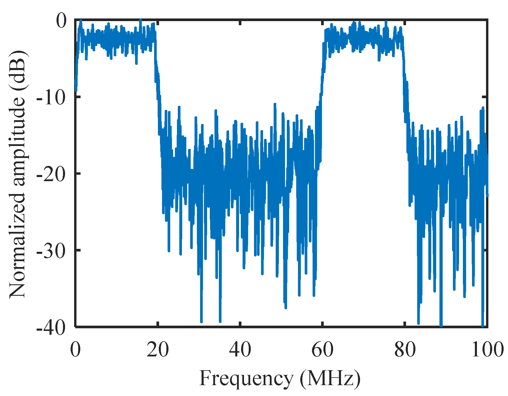
4. Results and Analyses

In this section, simulation experiments performed in MATLAB, and measured active interference data, were used to analyze and verify the interference behavior prediction performance of the proposed algorithm. To present the optimal performance of the proposed method, the noise in the interference parameter estimation results was ignored in the following numerical experiments. In practice, the influence of noise on prediction results could be mitigated by training in the presence of noise or introducing advanced training technology that could enhance the robustness of the prediction model [33,34].
For the analysis of the interference behavior prediction in the frequency domain, the available maximum bandwidth and the minimum working bandwidth of the radar system were assumed to be 100 MHz and 20 MHz, respectively, so 5 subchannels were divided in the frequency domain. Four active interference schemes were used to verify the interference frequency state prediction performance of the OS-ELM-FP algorithm. The specific active interference schemes in the frequency domain are shown in Table 1.
For the analysis of the interference behavior prediction in the spatial domain, both simulation data and measured data were used to verify the performance of the OS-ELM-AP algorithm. Specifically, the simulated interference angle data were generated based on the simulated missile trajectory. A ship target was assumed to move in the horizontal plane with the initial geodetic coordinate (6000, 7504, 0) m, a speed of 15 m/s and a direction of −120°. The active interference was inboard, so its movement was consistent with that of the ship target. The starting point of the missile was at the geodetic coordinate of (0, 0, 1500) m, the flight speed of the missile was vm = 300 m/s, the initial azimuth angle of the missile was o h x = 30 , and the initial pitch angle was o f y = 0 . The radar sensor was turned on to obtain the interference angle data when the missile-target distance was 10 km. The measured angle data of active interference were obtained by multichannel array radar in a sea-surface target detection experiment. The specific experimental settings are given in Section 4.3.
The comparison algorithms used in this section included GRP-based [19] interference behavior prediction and LSTM-based [21] interference behavior prediction. The two comparison algorithms were implemented based on MATLAB’s toolkit. The parameter settings of the prediction methods are given in Table 2, Table 3 and Table 4.
Based on the prediction models described in the above tables, the performance of the algorithms was verified from four aspects: online single-time interference behavior prediction performance, continuous multi-time interference behavior prediction performance, computational complexity and cognitive anti-interference performance based on the prediction results.

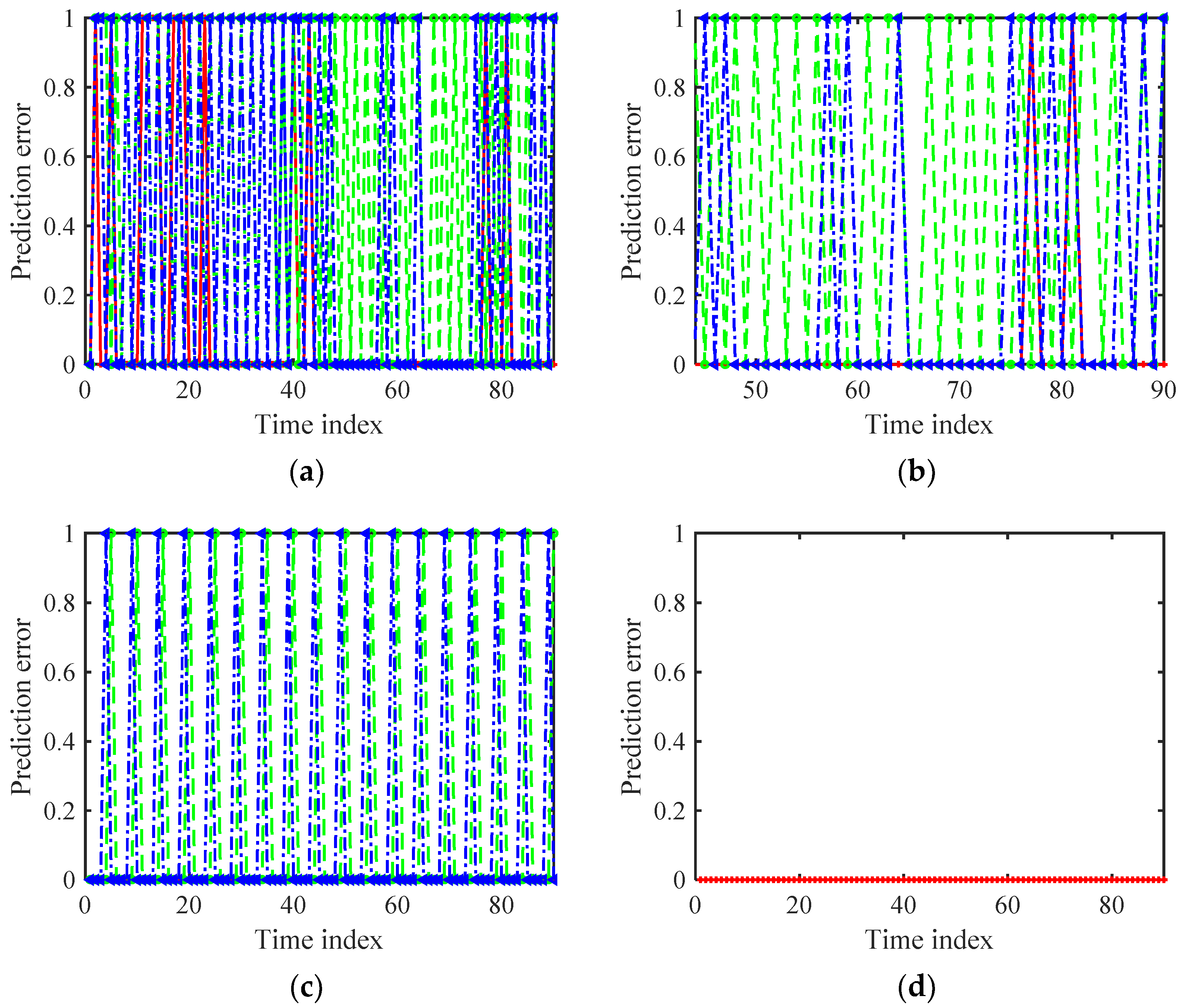
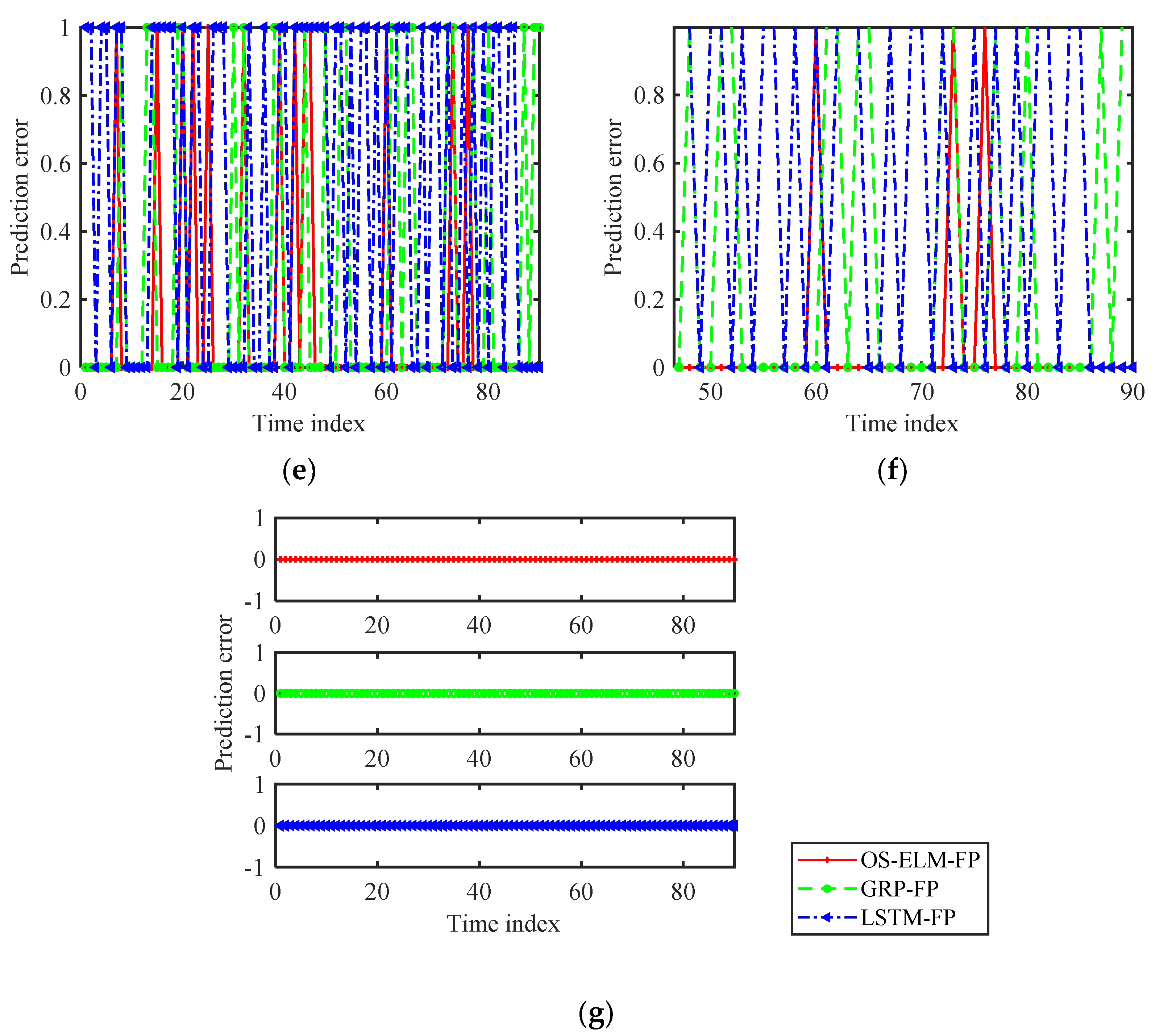
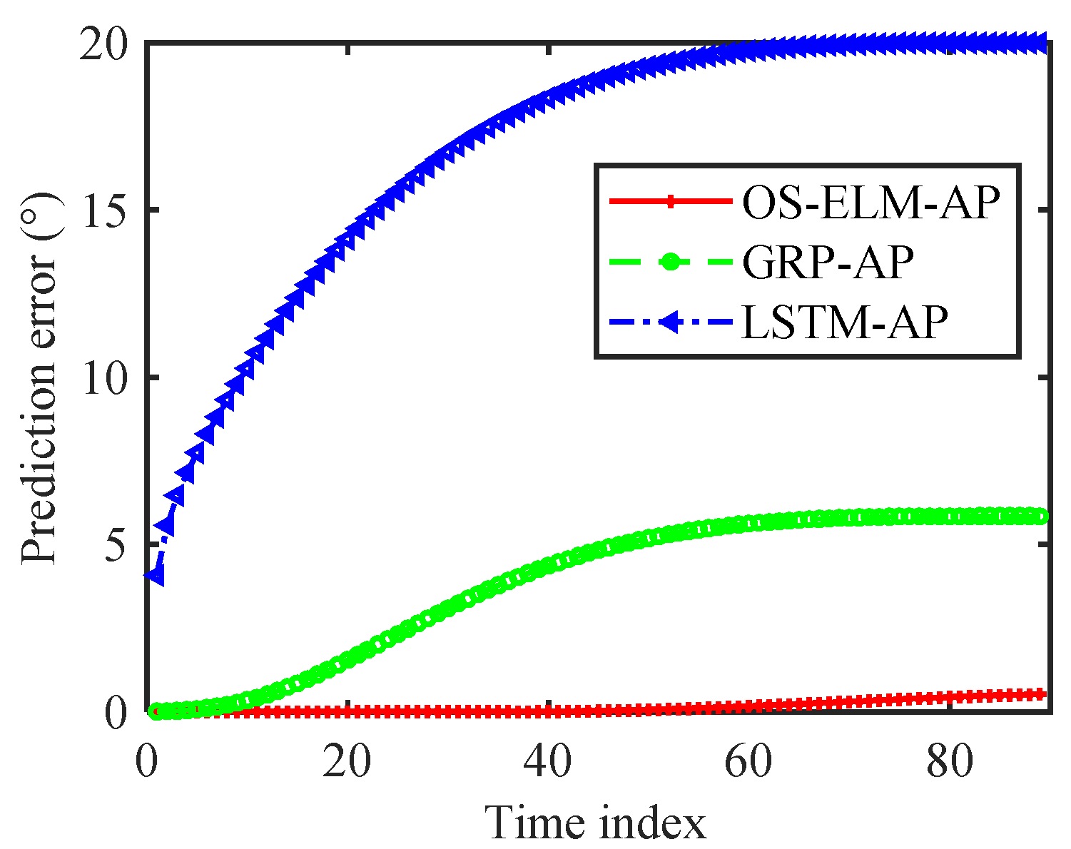
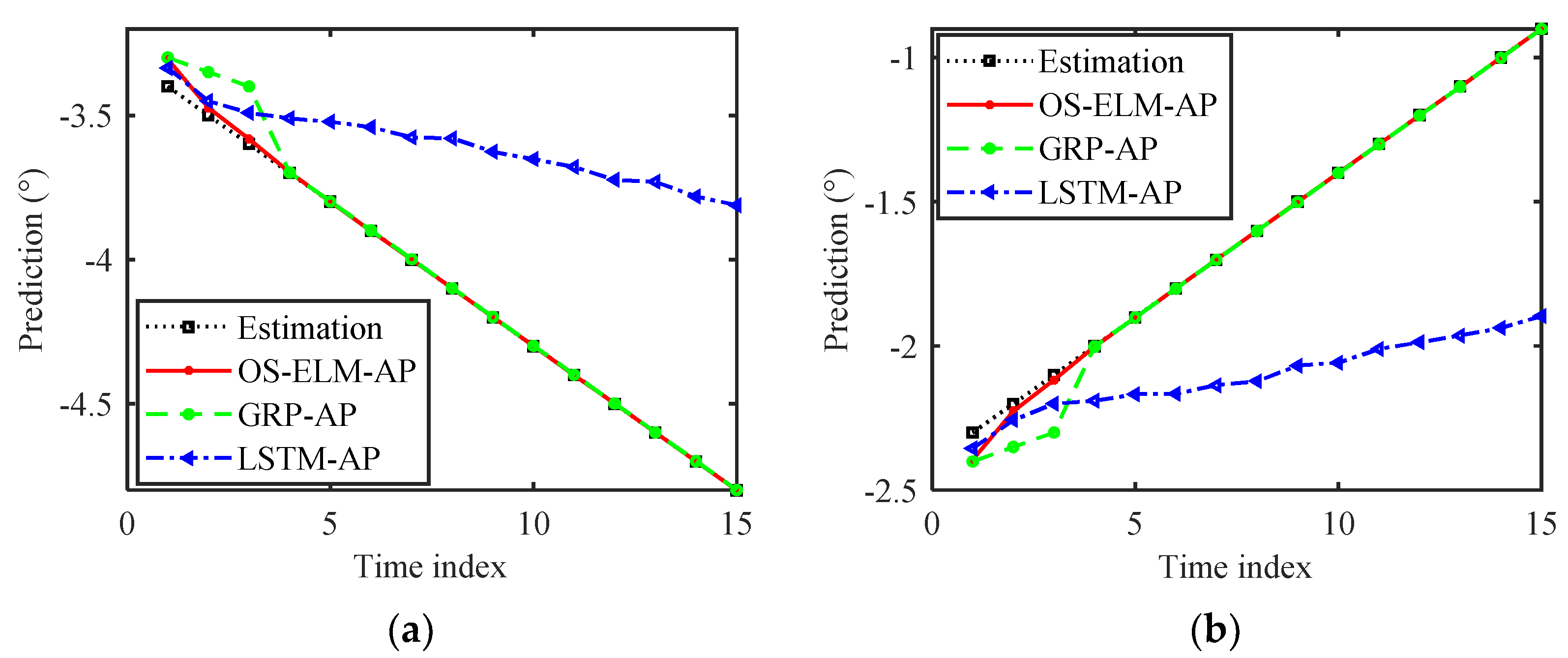
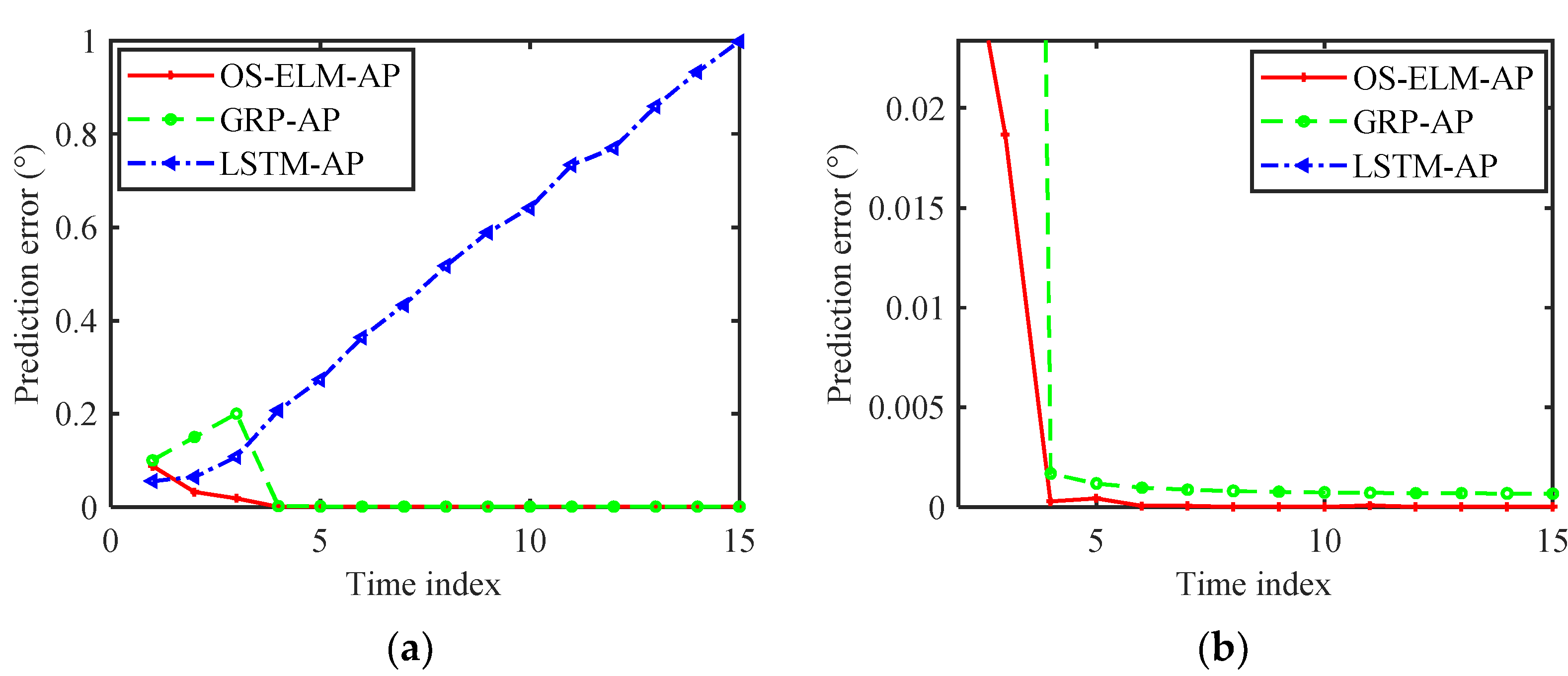
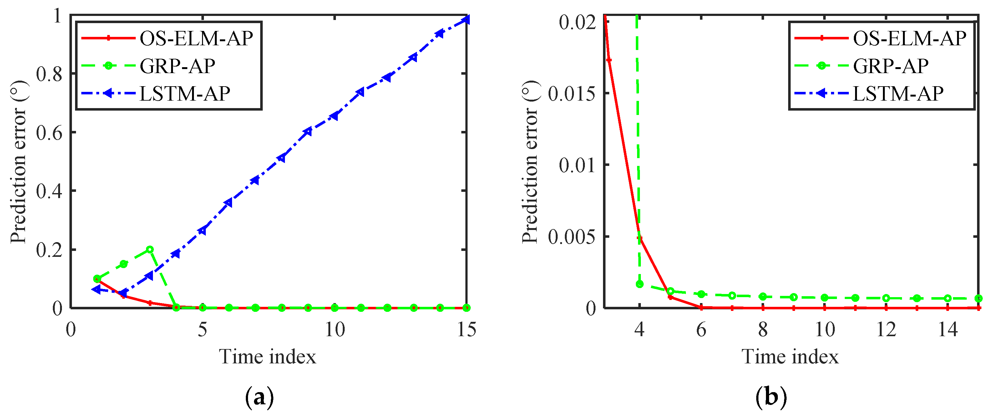
4.1. Analysis of the Single-Time Prediction Performance

Based on the time series of the interference angle obtained by the simulated ballistic trajectory, the single-time online prediction results obtained by different angle prediction algorithms are shown in Figure 7. The OS-ELM-AP and GRP-AP algorithms had significantly smaller prediction errors than the LSTM-AP algorithm. This was because only the time series of length 10 was used for prediction model training in the offline training phase, and the training dataset was only updated by one sample at an updating time in the online test phase. As a deep learning algorithm, small samples cannot guarantee the performance of LSTM-AP. For noncooperative active interference countermeasure applications with high real-time requirements, it is obvious that the available effective training data are limited. Therefore, as a single-layer feedforward neural network, OS-ELM-AP was more suitable for predicting noncooperative active interference activity than the LSTM-AP method. In addition, Figure 7b shows that the OS-ELM-AP algorithm achieved a better prediction performance than the GRP-AP algorithm.
In Figure 8, the active interference frequency state prediction results are given. Since the interference spectrum was represented by a binary vector, the prediction error was zero or one. The results show that for the interference frequency scheme generated by the two-state Markov process, the prediction errors obtained by the LSTM-FP algorithm and the OS-ELM-FP algorithm decreased with the updating model during the online test process, compared with those obtained by the GRP-FP algorithm. Specifically, for the 45 predictions starting from the 45th test, the LSTM-FP algorithm generated a total of 11 prediction errors, and the OS-ELM-FP algorithm had a total of 2 prediction errors. For the triangular sweep interference mode, the OS-ELM-FP algorithm had zero prediction errors in the test phase. This means that, based on a small number of offline training samples, the OS-ELM-FP algorithm successfully learned the scheme of the triangular sweep interference. In contrast, the GRP-FP algorithm and the LSTM-FP algorithm did not fully learn the interference behavior during the offline training process and could not accurately predict the interference state in the frequency domain based on online updating. In fact, the incorrect prediction results in Figure 8c appeared in the idle-busy transition state. Therefore, compared with the GRP-FP algorithm and the LSTM-FP algorithm, the proposed OS-ELM-FP algorithm could maintain a higher prediction accuracy for the interference state at the turning point. For stochastic interference, Figure 8e shows that the prediction performance of the GRP-FP algorithm and the LSTM-FP algorithm decreased with the increasing time delay of the online test data. In contrast, the proposed OS-ELM-FP algorithm could effectively improve the prediction performance by updating the prediction model parameters online. Specifically, for the 45 subsequent predictions, starting from the 45th test, the GRP-FP algorithm obtained a total of 13 prediction errors, the LSTM-FP algorithm made a total of 23 prediction errors and the OS-ELM-FP algorithm generated a total of 3 prediction errors. Finally, the prediction results of the three prediction algorithms in the barrage interference environment are given in Figure 8g. The three prediction algorithms could successfully learn the interference frequency behavior in this constant frequency scheme.
Then, we analyzed the cost time of the numerical examples in Figure 7 and Figure 8. The online update time of the prediction models is given in Table 5. As shown, the online update time of the OS-ELM-based method was much smaller than the online update times of the GRP and LSTM algorithms in both interference angle and frequency predictions. The main calculation complexity of the OS-ELM-based algorithm came from the pseudoinversion operation in the updating formula. Since the OS-ELM-based prediction model was updated based on a single sample in the online test phase, its computational complexity depended mainly on the hidden layer dimension L , i.e., o ( L 3 ) . The GRP-based prediction algorithm updated the model parameters with accumulated samples and could not achieve multichannel predictions in parallel. Therefore, with the increase in the number of samples N and the number of channels M , the computational complexity of the GRP-based method would increase greatly. Specifically, the computational complexity of the GRP-based method was o ( M N 3 ) . For the LSTM-based method, the computational complexity was o ( N I ( K N H + K C S + N H I + C S I ) ) , where N I , K , N H and C were the numbers of training iterations, output units, hidden layer units, and memory element blocks, respectively, S was the size of memory element blocks, and I was the number of units connecting the memory elements, gate units, and hidden layer. Compared with the OS-ELM with a single hidden layer, the LSTM structure was more complex and, hence, resulted in greater calculation complexity in the updating process.

4.2. Analysis of the Continuous Multitime Prediction Performance

In the active interference countermeasure scenario, due to the noncooperative property of active interference and the uncertainty of other environmental factors in the perception process, the sensed effective active interference data might be interrupted. Therefore, it was of great significance to design a prediction algorithm with good continuous multi-time prediction performance. The multi-time prediction results of the active interference angle with different algorithms are shown in Figure 9. The later the time of the sample to be predicted, the larger the prediction error would be. This was because the prediction error accumulated in the continuous multi-time prediction. Nevertheless, Figure 9 shows that the OS-ELM-AP algorithm could keep the interference angle prediction errors within 0.01° in the first 41 consecutive predictions. This was much better than the GRP algorithm and the LSTM algorithm.
In Figure 10, the continuous multi-time prediction results of the active interference frequency state are given. Since there was no online update process in the continuous multi-time prediction, for the triangular sweep frequency mode, the OS-ELM-FP algorithm made prediction errors at the idle-busy transition points similar to the other two prediction algorithms. In the barrage interference environment, the three algorithms could accurately predict the interference state in the continuous multi-time prediction. For the stochastic interference case, the multi-time prediction performance of the OS-ELM-FP algorithm was better than that of the other two methods.
The average multi-time prediction errors of different algorithms are given in Table 6 by counting the interference behavior prediction results at 90 consecutive moments. The interference azimuth prediction error of OS-ELM-AP was much smaller than that of the other two methods. For the interference frequency state prediction, the average continuous multi-time prediction error of the OS-ELM-FP was consistent with that of the other two methods in the cases of the Markov-process-based interference mode, the triangular sweep interference mode, and the barrage interference mode. For stochastic interference, the average prediction error of the OS-ELM-FP method was smaller than that of the other methods. The results in the table further highlight the superiority of the OS-ELM-based active interference activity prediction method in multi-time prediction scenarios.

4.3. Analysis of Interference Activity Prediction Performance Based on Measured Data

This subsection analyzes and verifies the performance of the OS-ELM-AP based on the measured data. The experimental scenario is shown in Figure 11. The target used for calibration was within the range of the radar transmit beam, and the ship carrying an active jammer entered the irradiation range of the radar system along Path 1 from the right side of the beam. After reaching the designated position, the ship returned along Path 2.
Under the above experimental conditions, the interference azimuth data in Path 1 and Path 2 were measured. Based on this collected interference azimuth data, the prediction results of different methods are shown in Figure 12, and the prediction errors are given in Figure 13 and Figure 14. As shown, the prediction performance of the LSTM-AP algorithm was poor due to the small number of samples. Both the OS-ELM-AP algorithm and GRP-AP algorithm could achieve better prediction performance with online updating. Specifically, after four online updates, the prediction errors of the OS-ELM-AP algorithm and the GRP-AP algorithm were less than 0.005°. In addition, Figure 13b and Figure 14b show that starting from the fifth online test, the jammer angle prediction error generated by the OS-ELM-AP algorithm was smaller than that generated by the GRP-AP algorithm.

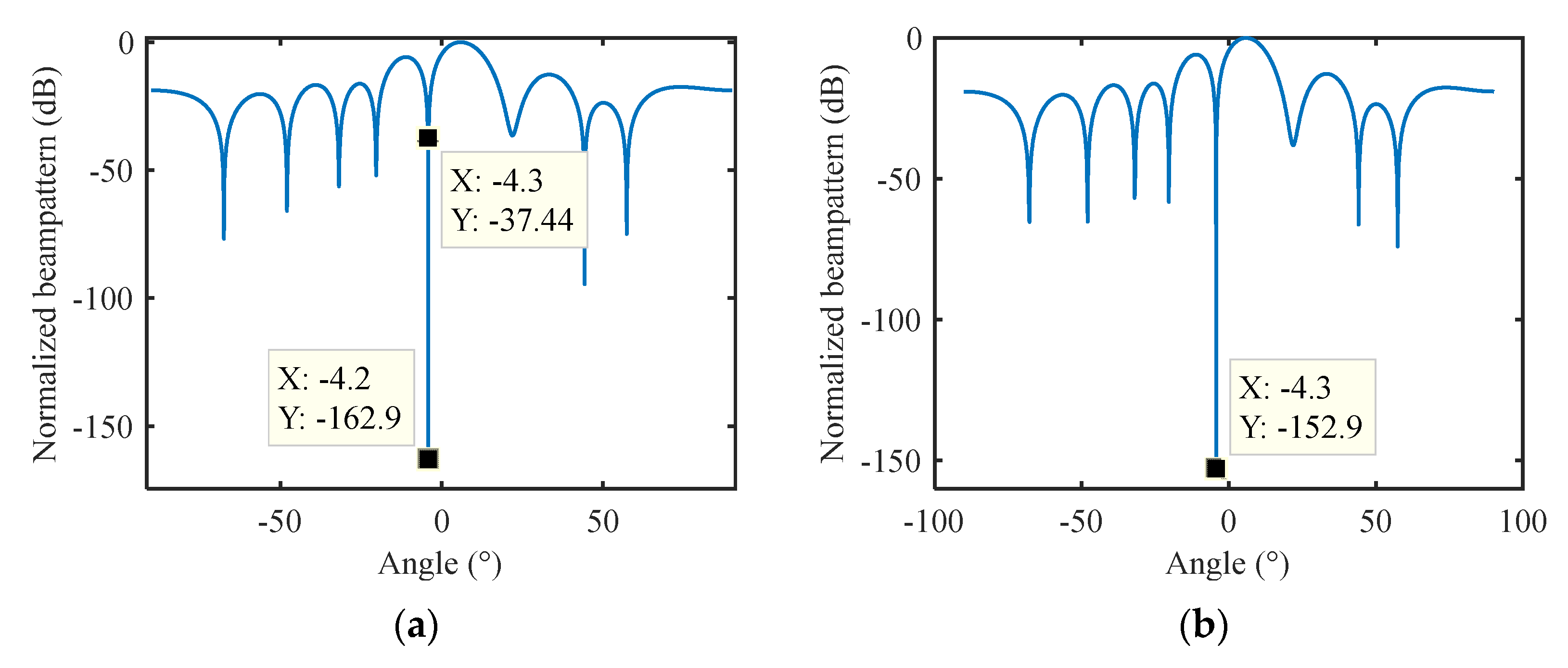
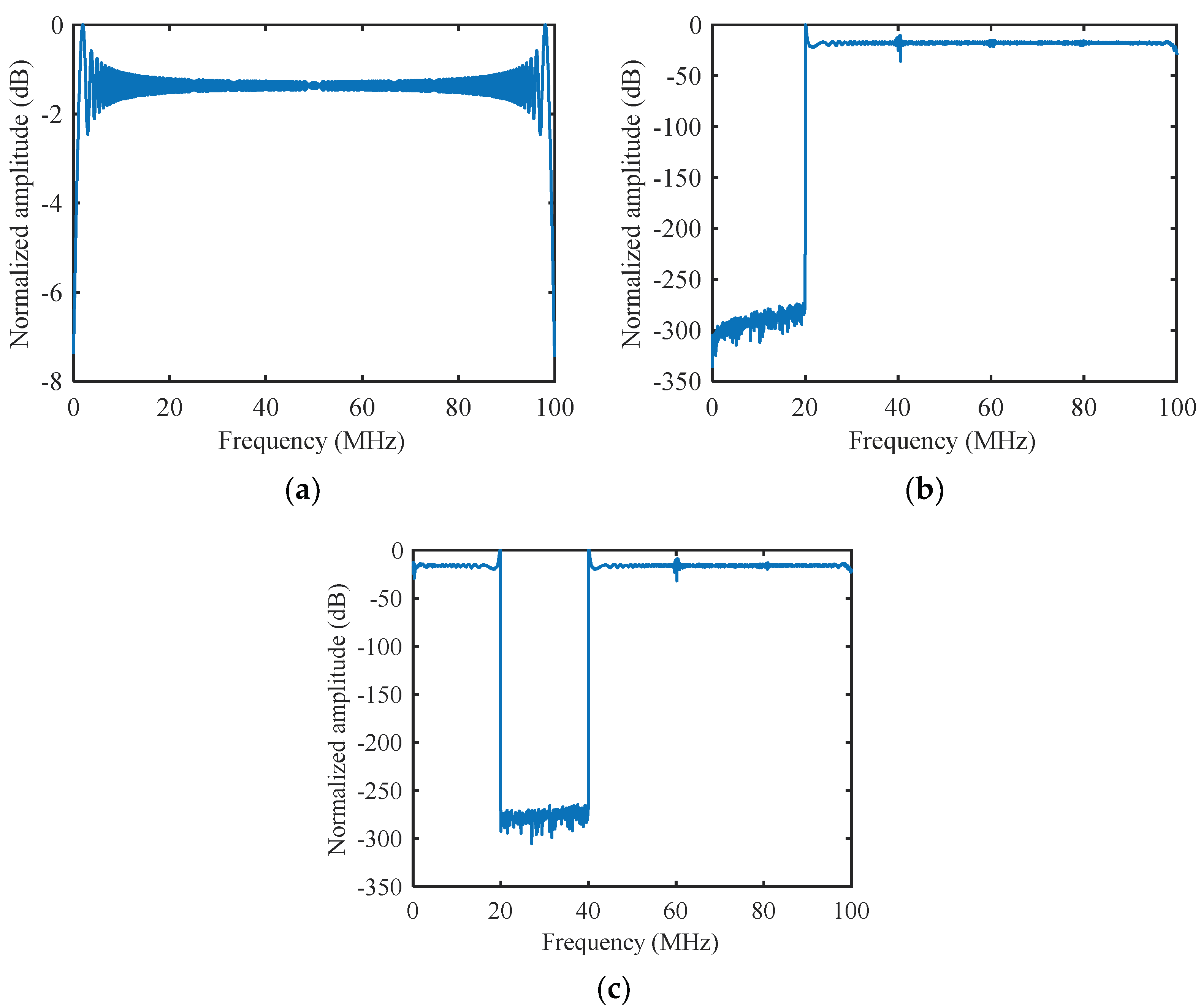
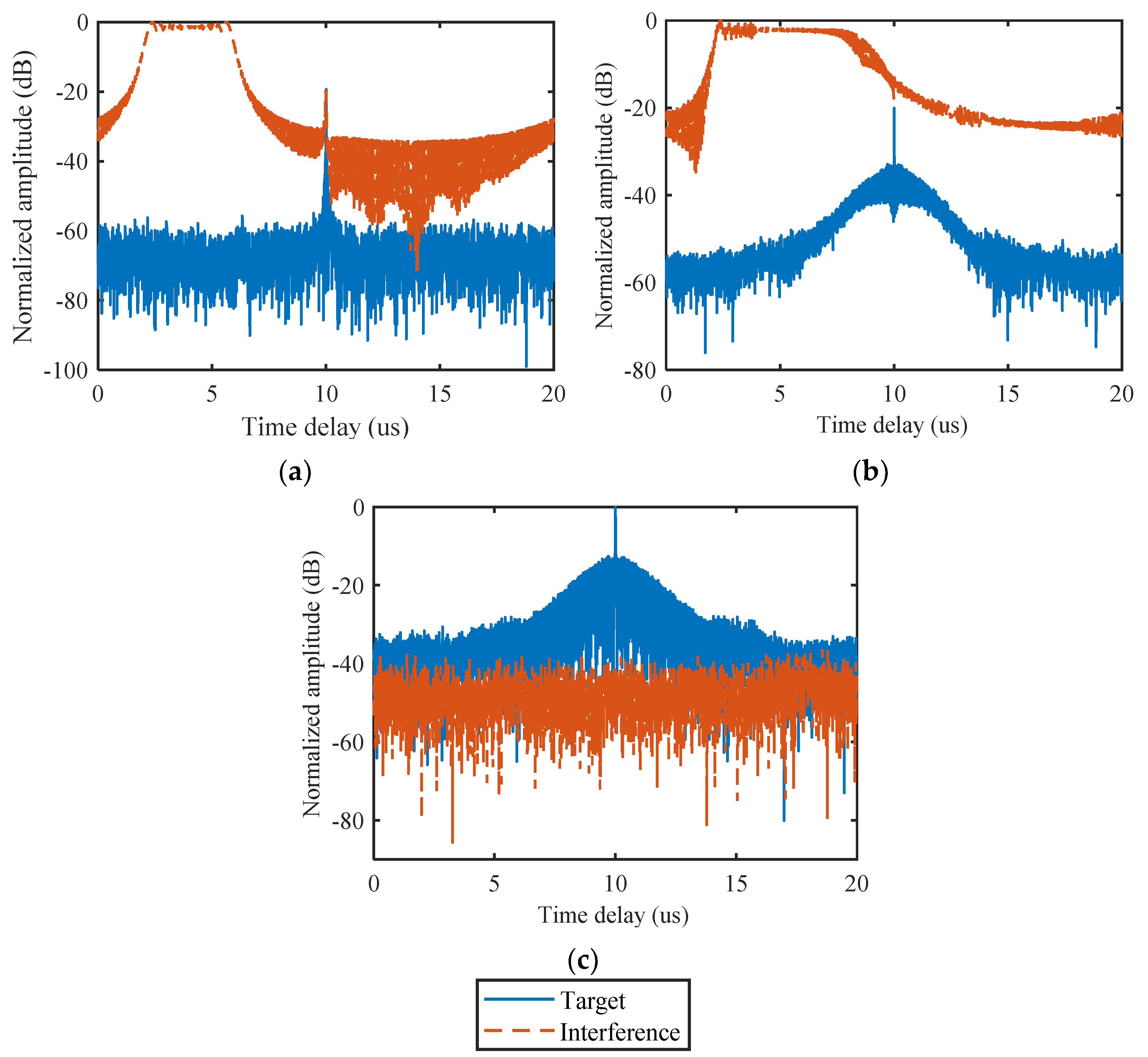
4.4. Analysis of the Anti-Active Interference Performance Based on Interference Activity Predictions

This subsection illustrates the boosting effect of the proposed interference behavior prediction method on the cognitive anti-interference performance. For cognitive anti-interference in the spatial domain, the radar system designs the transmitting beam with notches formed in the interference direction to reduce the probability of the radar signal being intercepted by enemy jammers and suppresses the electromagnetic interference to other equipment. Therefore, we measured the spatial cognitive anti-interference performance by the transmit beam nulling level in the interference azimuth. For cognitive anti-interference in the frequency domain, the transmit waveform design is usually combined with the receiver filter to counter active interference. Therefore, we assessed the cognitive anti-interference performance in the frequency domain by the output signal-to-interference ratio (SIR) of the receiver filter.
The transmit beams synthesized using the sensed and predicted results of the 10th sample in Figure 12a are shown in Figure 15a,b, respectively. The actual interference angle corresponding to the 10th sample was −4.3°, the sensed result was −4.2°, and the prediction result was −4.3°. The nulling level of the transmitted beam at the true interference azimuth was −37.44 dB, based on the sensed interference information, while the formed nulling level was −152.9 dB with the predicted interference angle. Obviously, the interference behavior prediction based on OS-ELM-AP could effectively improve the cognitive anti-interference performance in the spatial domain.
The spectrum of the traditional chirp signal with a bandwidth of 100 MHz is given in Figure 16a. The active interference was composed of multicarrier signals, and the signal-to-noise ratio (SNR) and the interference-to-noise ratio (INR) of the received signal were 10 dB and 50 dB, respectively. By using the perception and prediction frequency results of the triangular sweep interference in Figure 8c, the spectra of the designed cognitive transmit waveforms are shown in Figure 16b,c. Corresponding to the interference frequency perception results, the designed transmit waveform was null at 0-20 MHz. Through OS-ELM-FP-based interference frequency prediction, it could be learned that interference occupied the second frequency subchannel. With the prediction result, the cognitive radar system designed a transmit waveform with a notch at 20-40 MHz.
Following the transmit waveforms in Figure 16, the corresponding output results of the matched filter are shown in Figure 17. In the two cases of transmitting the chirp signal and transmitting the cognitive anti-interference signal designed, based on the sensed interference frequency state, the output target echo was completely suppressed by the active interference signal. In contrast, using the interference frequency information predicted based on OS-ELM-FP to design the anti-interference waveform could effectively improve the output SIR. Specifically, the SIRs obtained by the chirp signal, the waveform designed based on the sensed interference frequency state and the waveform designed according to the OS-ELM-FP-based prediction result were −19.4 dB, −20 dB and 36.8 dB, respectively. Therefore, the proposed OS-ELM-FP could effectively optimize the cognitive anti-interference capability by improving the effectiveness of the active interference information.

5. Conclusions

In this paper, an OS-ELM-based method that contains interference frequency and angle prediction models, i.e., OS-ELM-AP and OS-ELM-FP, is proposed for active interference activity prediction in cognitive radar. Due to the flexible single-hidden-layer network structure and recursive-formula-based output weight updating, the interference state in multiple frequency channels can be simultaneously predicted efficiently and accurately by the proposed OS-ELM-FP method. Furthermore, based on the current interference direction estimates, the future interference angle can be efficiently predicted by the proposed OS-ELM-AP model, and the cognitive anti-interference performance is, thus, improved. The proposed method can achieve smaller prediction errors with a low computational complexity than state-of-the-art methods, which has been verified by simulation and measured interference data.
Considering the intelligence of active interference and extending the method to a multiagent application are future research directions of this work.

Author Contributions

Conceptualization, S.W.; methodology, Z.L. and S.W.; software, S.W.; validation, S.W., L.R. and R.X.; formal analysis, S.W.; investigation, S.W., L.R.; writing—original draft preparation, S.W.; writing—review and editing, L.R.; supervision, Z.L. All authors have read and agreed to the published version of the manuscript.

Funding

This research was funded by the National Natural Science Foundation of China, grant number 62001346.

Conflicts of Interest

The authors declare no conflict of interest.

References

  1. Ding, L.; Li, R.; Wang, Y.; Dai, L.; Chen, F. Discrimination and identification between mainlobe repeater jamming and target echo by basis pursuit. IET Radar Sonar Navig. 2017, 11, 11–20. [Google Scholar] [CrossRef]
  2. Chen, X.; Shu, T.; Yu, K.-B.; Zhang, Y.; Lei, Z.; He, J.; Yu, W. Implementation of an adaptive wideband digital array radar processor using subbanding for enhanced jamming cancellation. IEEE Trans. Aerosp. Electron. Syst. 2021, 57, 762–775. [Google Scholar] [CrossRef]
  3. Yu, H.; Liu, N.; Zhang, L.; Li, Q.; Zhang, J.; Tang, S.; Zhao, S. An Interference suppression method for multistatic radar based on noise subspace projection. IEEE Sens. J. 2020, 20, 8797–8805. [Google Scholar] [CrossRef]
  4. Govoni, M.A.; Li, H.; Kosinski, J.A. Low probability of interception of an advanced noise radar waveform with Linear-FM. IEEE Trans. Aerosp. Electron. Syst. 2013, 49, 1351–1356. [Google Scholar]
  5. Tang, B.; Naghsh, M.M.; Tang, J. Relative entropy-based waveform design for MIMO radar detection in the presence of clutter and interference. IEEE Trans. Signal Process. 2015, 63, 3783–3796. [Google Scholar] [CrossRef]
  6. Wang, S.; Liu, Z.; Xie, R.; Ran, L.; Wang, J. MIMO radar waveform design for target detection in the presence of interference. Digit. Signal Process. 2021, 114, 103060. [Google Scholar] [CrossRef]
  7. Aubry, A.; Carotenuto, V.; De Maio, A.; Farina, A.; Pallotta, L. Optimization theory-based radar waveform design for spectrally dense environments. IEEE Aerosp. Electron. Syst. Mag. 2016, 31, 14–25. [Google Scholar] [CrossRef]
  8. Li, K.; Jiu, B.; Liu, H.; Pu, W. Robust antijamming strategy design for frequency-agile radar against main lobe jamming. Remote Sens. 2021, 13, 3043. [Google Scholar] [CrossRef]
  9. Thornton, C.E.; Kozy, M.A.; Buehrer, R.M.; Martone, A.F.; Sherbondy, K.D. Deep reinforcement learning control for radar detection and tracking in congested spectral environments. IEEE Trans. Cogn. Commun. Netw. 2020, 6, 1335–1349. [Google Scholar] [CrossRef]
  10. Wang, S.; Liu, Z.; Xie, R.; Ran, L. Reinforcement learning for compressed-sensing based frequency agile radar in the presence of active interference. Remote Sens. 2022, 14, 968. [Google Scholar] [CrossRef]
  11. Chung, H.; Kang, J.; Kim, H.; Park, Y.M.; Kim, S. Adaptive beamwidth control for mmwave beam tracking. IEEE Commun. Lett. 2021, 25, 137–141. [Google Scholar] [CrossRef]
  12. Blandino, S.; Bertrand, T.; Desset, C.; Bourdoux, A.; Pollin, S.; Louveaux, J. A blind beam tracking scheme for millimeter wave systems. In Proceedings of the IEEE 91st Vehicular Technology Conference (VTC2020-Spring), Antwerp, Belgium, 25–28 May 2020; pp. 1–6. [Google Scholar] [CrossRef]
  13. Agarwal, A.; Gangopadhyay, R.; Dubey, S.; Debnath, S.; Khan, M.A. Learning-based predictive dynamic spectrum access framework: A practical perspective for enhanced QoE of secondary users. IET Commun. 2018, 12, 2243–2252. [Google Scholar] [CrossRef]
  14. Eltom, H.; Kandeepan, S.; Moran, B.; Evans, R.J. Spectrum occupancy prediction using a hidden Markov model. In Proceedings of the International Conference on Signal Processing and Communication Systems (ICSPCS), Cairns, QLD, Australia, 14–16 December 2015. [Google Scholar]
  15. Sharma, M.; Sahoo, A. Stochastic model based opportunistic channel access in dynamic spectrum access networks. IEEE Trans. Mob. Comput. 2014, 13, 1625–1639. [Google Scholar] [CrossRef]
  16. Kovarskiy, J.A. Comparing stochastic and Markov decision process approaches for predicting radio frequency interference. In Proceedings of the Radar Sensor Technol. XXIII, Baltimore, MD, USA, 15–17 April 2019. [Google Scholar]
  17. Martone, A.F. Metacognition for radar coexistence. In Proceedings of the IEEE International Radar Conference, Washington, DC, USA, 28–30 April 2020; pp. 55–66. [Google Scholar] [CrossRef]
  18. Stinco, P.; Greco, M.; Gini, F.; Himed, B. Cognitive radars in spectrally dense environments. IEEE Aerosp. Electron. Syst. Mag. 2016, 31, 20–27. [Google Scholar] [CrossRef]
  19. Kovarskiy, J.A.; Kirk, B.H.; Martone, A.F.; Narayanan, R.M.; Sherbondy, K.D. Evaluation of real-time predictive spectrum sharing for cognitive radar. IEEE Trans. Aerosp. Electron. Syst. 2021, 57, 690–705. [Google Scholar] [CrossRef]
  20. Song, H.-L.; Ko, Y.-C. Beam alignment for high-speed UAV via angle prediction and adaptive beam coverage. IEEE Trans. Veh. Technol. 2021, 70, 10185–10192. [Google Scholar] [CrossRef]
  21. Shawel, B.S.; Woldegebreal, D.H.; Pollin, S. Convolutional LSTM-based long-term spectrum prediction for dynamic spectrum access. In Proceedings of the 27th European Signal Processing Conference (EUSIPCO), A Coruna, Spain, 2–6 September 2019; pp. 1–5. [Google Scholar]
  22. Radhakrishnan, N.; Kandeepan, S. An improved initialization method for fast learning in long short-term memory-based markovian spectrum prediction. IEEE Trans. Cogn. Commun. Netw. 2021, 7, 729–738. [Google Scholar] [CrossRef]
  23. Huang, G.; Huang, G.B.; Song, S.; You, K. Trends in extreme learning machines: A review. Neural Netw. 2015, 61, 32–48. [Google Scholar] [CrossRef]
  24. Huang, G.-B.; Zhu, Q.-Y.; Siew, C.-K. Extreme learning machine: Theory and applications. Neurocomputing 2006, 70, 489–501. [Google Scholar] [CrossRef]
  25. Huang, G.; Song, S.; Gupta, J.N.D.; Wu, C. Semi-supervised and unsupervised extreme learning machines. IEEE Trans. Cybern. 2014, 44, 2405–2417. [Google Scholar] [CrossRef]
  26. Benoît, F.; van Heeswijk, M.; Miche, Y.; Verleysen, M.; Lendasse, A. Feature selection for nonlinear models with extreme learning machines. Neurocomputing 2013, 102, 111–124. [Google Scholar] [CrossRef]
  27. Li, Y.; Gu, X.P. Application of online SVR in very short-term load forecasting. Int. Rev. Electr. Eng. 2013, 8, 277–282. [Google Scholar]
  28. Liang, N.-Y.; Huang, G.-B.; Saratchandran, P.; Sundararajan, N. A fast and accurate online sequential learning algorithm for feedforward networks. IEEE Trans. Neural Netw. 2006, 17, 1411–1423. [Google Scholar] [CrossRef]
  29. Zheng, J.; Yang, T.; Liu, H.; Su, T. Efficient data transmission strategy for IIoTs with arbitrary geometrical array. IEEE Trans. Ind. Informatics 2021, 17, 3460–3468. [Google Scholar] [CrossRef]
  30. Martone, A.F.; Ranney, K.I.; Sherbondy, K.; Gallagher, K.A.; Blunt, S.D. Spectrum allocation for noncooperative radar coexistence. IEEE Trans. Aerosp. Electron. Syst. 2018, 54, 90–105. [Google Scholar] [CrossRef]
  31. Zheng, J.; Yang, T.; Liu, H.; Su, T.; Wan, L. Accurate detection and localization of unmanned aerial vehicle swarms-enabled mobile edge computing system. IEEE Trans. Ind. Inform. 2021, 17, 5059–5067. [Google Scholar] [CrossRef]
  32. Zheng, J.; Chen, R.; Yang, T.; Liu, X.; Liu, H.; Su, T.; Wan, L. An efficient strategy for accurate detection and localization of UAV swarms. IEEE Internet Things J. 2021, 8, 15372–15381. [Google Scholar] [CrossRef]
  33. Zhang, M.; Qu, H.; Xie, X.; Kurths, J. Supervised learning in spiking neural networks with noise-threshold. Neurocomputing 2017, 219, 333–349. [Google Scholar] [CrossRef] [Green Version]
  34. Yang, Y.; Xiang, W. Robust optimization framework for training shallow neural networks using reachability method. In Proceedings of the 60th IEEE Conference on Decision and Control (CDC), Austin, TX, USA, 14–17 December 2021; pp. 3857–3862. [Google Scholar] [CrossRef]
Figure 1. Anti-interference framework of cognitive radar.
Remotesensing 14 02737 g001
Figure 2. Block diagram of the active interference activity prediction in the frequency domain.
Remotesensing 14 02737 g002
Figure 3. Block diagram of interference spectrum coding.
Remotesensing 14 02737 g003
Figure 4. Interference spectrum coding example.
Remotesensing 14 02737 g004
Figure 5. OS-ELM-FP-based interference frequency prediction network.
Remotesensing 14 02737 g005
Figure 6. OS-ELM-AP-based interference angle prediction network.
Remotesensing 14 02737 g006
Figure 7. Online single-time interference angle prediction results. (a) Angle prediction error. (b) Magnified view of (a).
Remotesensing 14 02737 g007
Figure 8. Online single-time interference frequency prediction results. (a) Prediction error for the Markov case. (b) Magnified view of (a). (c) Prediction error for the triangular sweep case. (d) Magnified view of (c). (e) Prediction error for the stochastic case. (f) Magnified view of (e). (g) Prediction error for the barrage case.
Remotesensing 14 02737 g008aRemotesensing 14 02737 g008b
Figure 9. Online continuous multi-time angle prediction results.
Remotesensing 14 02737 g009
Figure 10. Online continuous multi-time frequency prediction results for the (a) Markov, (b) triangular sweep, (c) stochastic and (d) barrage interference schemes.
Remotesensing 14 02737 g010
Figure 11. Experimental scenario.
Remotesensing 14 02737 g011
Figure 12. Online angle prediction results for (a) Path 1 and (b) Path 2.
Remotesensing 14 02737 g012
Figure 13. Online angle prediction errors for Path 1. (a) Prediction errors. (b) Magnified view of (a).
Remotesensing 14 02737 g013
Figure 14. Online angle prediction errors for Path 2. (a) Prediction errors. (b) Magnified view of (a).
Remotesensing 14 02737 g014
Figure 15. Transmit beampattern synthesized using (a) sensed and (b) predicted interference knowledge.
Remotesensing 14 02737 g015
Figure 16. Normalized spectra of the (a) LFM waveform, (b) waveform designed using sensed interference information and (c) waveform designed using the OS-ELM-FP-based interference frequency prediction.
Remotesensing 14 02737 g016
Figure 17. Outputs of the matched filter for the (a) LFM waveform, (b) waveform designed using sensed interference information, and (c) waveform designed using the OS-ELM-FP-based interference frequency prediction result.
Remotesensing 14 02737 g017
Table 1. Active interference activity schemes in the frequency domain.
InterferenceScheme
MarkovOccupies each frequency subchannel according to the two-state Markov process defined as:
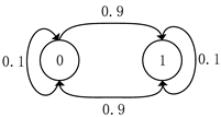
 Remotesensing 14 02737 i001.
Triangular sweepSweeps over the available frequency bands with triangular behavior.
BarrageOccupies all the frequency channels.
StochasticOccupies the 5 frequency subchannels with probabilities [0.5 0.3 0.1 0.1 0].
Table 2. Parameter setting of the GRP-based interference activity prediction model.
Signal DomainOffline Training Set SizeInput/Output SizeKernel FunctionInitial Noise Standard DeviationSignal Standard DeviationFeature Length Scale
Space101square exponential0.23.56.2
Frequency101square exponential0.23.56.2
Table 3. Parameter setting of the LSTM-based interference activity prediction model.
Signal DomainOffline Training Set SizeInput/Output SizeHidden Layer SizeSolution MachineIterationsInitial Learning RateReduction Factor of Learning Rate
Space10110‘adam’2500.0050.2
Frequency10510‘adam’2500.0050.2
Table 4. Parameter setting of the OS-ELM-based interference activity prediction model.
Signal DomainOffline Training Set SizeInput/Output SizeTransfer FunctionHidden Layer Size
Space101Sigmoid10
Frequency105Sigmoid10
Table 5. Numerical examples of the cost time.
AlgorithmOnline Update Time of Angle Prediction (s)Online Update Time of Frequency Prediction (s)
OS-ELM-AP/FP0.00160.0017
GRP-AP/FP0.10380.9510
LSTM-AP/FP3.78353.8407
Table 6. Average continuous multi-time prediction error.
AlgorithmAngle Prediction ErrorFrequency Prediction Error
MarkovTriangular SweepStochasticBarrage Interference
OS-ELM-AP/FP0.1340°0.51110.20000.14440
GRP-AP/FP3.8678°0.51110.20000.24440
LSTM-AP/FP16.8456°0.51110.20000.50000
Publisher’s Note: MDPI stays neutral with regard to jurisdictional claims in published maps and institutional affiliations.

