Article

Attribution of NDVI Dynamics over the Globe from 1982 to 2015

1
Laboratory of Critical Zone Evolution, School of Geography and Information Engineering, China University of Geosciences, Wuhan 430074, China
2
State Key Laboratory of Hydrology-Water Resources and Hydraulic Engineering, Nanjing Hydraulic Research Institute, Nanjing 210098, China
3
Key Laboratory of Environmental Change and Natural Disaster, Ministry of Education, Beijing Normal University, Beijing 100875, China
4
State Key Laboratory of Earth Surface Processes and Resource Ecology, Beijing Normal University, Beijing 100875, China
5
Faculty of Geographical Science, Academy of Disaster Reduction and Emergency Management, Beijing Normal University, Beijing 100875, China
6
School of Urban, Resource and Environmental Sciences, Jiangsu Second Normal University, Nanjing 211200, China
7
Department of Atmospheric Science, School of Environmental Studies, China University of Geosciences, Wuhan 430074, China
8
Research Center of Ecology and Environment in Central Asia, Xinjiang Institute of Ecology and Geography, Chinese Academy of Sciences, Urumqi 830011, China
9
Institute of Water Problems, Hydropower and Ecology of the National Academy of Sciences of Tajikistan, Dushanbe 734042, Tajikistan
*
Author to whom correspondence should be addressed.
Remote Sens. 2022, 14(11), 2706; https://doi.org/10.3390/rs14112706
Submission received: 28 April 2022 / Revised: 28 May 2022 / Accepted: 2 June 2022 / Published: 4 June 2022
(This article belongs to the Special Issue Vegetation Biophysical Variables and Remote Sensing Applications)

Abstract

:
Satellite remote sensing has witnessed a global widespread vegetation greening since the 1980s. However, reliable observation-based quantitative knowledge on global greening remains obscure due to uncertainties in model simulations and the contribution of natural variability is largely unknown. Here, we revisit the attribution of global vegetation changes using the Time Series Segment and Residual Trend (TSS-RESTREND) method. Results showed global vegetation significantly greening over 40.6% of the vegetated grids, whereas vegetation significantly browning over 11.6% of the vegetated grids. The attribution results based on the TSS-RESTREND method show that CO2 fertilization (CO2) plays an influential role in vegetation changes over 61.4% of the global vegetated areas, followed by land use (LU, 23.5%), climate change (CC, 7.3%), and climate variability (CV, 1.5%). The vegetation greening can be largely attributed to CO2 fertilization while the vegetation browning is mainly caused by LU. Meanwhile, we also identify positive impacts of LU and CC on vegetation change in arid regions but negative impacts in humid regions. Our findings indicate spatial heterogeneity in causes behind global vegetation changes, providing more detailed references for global vegetation modeling.

1. Introduction

Vegetation plays a prominent role in the global hydrological and energy cycle via land-atmosphere interaction [1,2]. Global greening, defined as significantly increased vegetation, has been widely reported in recent years [3,4]. Vegetation change is a critical factor that profoundly affects global land carbon sink, global warming, the water cycle, and water resources [4]. In this context, a better quantitative understanding of the driving mechanism of global greening is requisite to achieve sustainable ecological management.
Currently, there is a widespread perception in the scientific literature and media coverage that the globe is becoming greener. Finding an explanation for this greening has attracted wide interest in recent years [4,5,6]. It has been theorized that anthropogenic climate change (CC) has profound impacts on vegetation greening over northern extratropical latitudes [7]. Based on the ecosystem models, Zhu et al. [3] found that CO2 fertilization (CO2) had the most significant effects on the observed greenness. However, the model-simulation based attributions in previous studies provided variable estimates, due to both spatiotemporal inaccuracies in driving data and simplified descriptions of human land use activities [4,8]. Chen et al. [5] pointed out that previous studies usually overestimate the CO2 fertilization effects and underestimate the direct influence of land use (LU) on vegetation greening. This limits our ability to develop a generic and unifying physically based understanding of global greening and predicting future vegetation change. Specifically, Song et al. [9] found that LU is the dominant factor of changes in the global woody and herbaceous vegetation coverage. All these papers pointed out the greening trends of global vegetation, yet the consensus has not been reached on the causes behind global greening.
Generally, vegetation changes can be affected by the complex interactions of atmospheric CO2 concentration, human LU, and climate [3,10]. However, due to the complex and nonlinear interactions among these factors and the weaknesses of current vegetation models, the fractional contribution of each factor to vegetation changes is still rather uncertain and yet to be quantified in a robust manner. Especially, climate variability (CV) can potentially drive vegetation changes [3,11]. Chen et al. [11] attributed interannual variability of greenness over 45% of global vegetated areas to CV. Burrell et al. [10] found that CV influenced vegetation greening over ~13% of global drylands areas. However, it is not well understood yet to what extent the global greenness change can be attributed to CV. In this case, we need more attempts to fully quantify the global greening drivers. Burrell et al. [12] proposed an observation-based attribution method for dryland degradation, i.e., Time Series Segment and Residual Trends (TSS-RESTREND). Observation-based attribution of global greening is theoretically critical in the mechanistic understanding of vegetation variations and ecological conservation in a changing climate. Different from model-based approaches which regulated LU [3] and relevant uncertainties [8], the TSS-RESTREND highlights the implications of CC and LU. Hence, this method has been widely used in attribution analysis [13,14,15]. Here, we apply the modified TSS-RESTREND method to perform an observation-based attribution of the vegetation greening across the globe. This research deeply analyzes the indispensable role of LU on global greenness change, considers the contribution of CV, and reveals fresh information about the potential drivers of vegetation change. Besides, this study provides spatially more comprehensive information about the regional difference in driving factors and the contribution of diverse land cover types on global vegetation change, compared to previous similar studies (i.e., Burrell et al. [10]) which mainly focused on the global and/or continental scale.
Overall, the scientific objectives of this study are to (1) estimate the trends of global vegetation greenness from 1982 to 2015; (2) quantify the detailed roles of CO2, LU, CC, and CV on greenness change; and (3) investigate the dominant factor controlling global vegetation changes. Altogether, we expect our analysis to add significant value in the ongoing discussion about the changing mechanisms of the terrestrial ecosystem and global vegetation modeling because it provides novel results that heavily rely on observations.

2. Materials and Methods

2.1. GIMMSv3.1g NDVI Data

Here we used the Global Inventory Monitoring and Modeling System Version 3 (GIMMSv3.1g) Normalized Difference Vegetation Index (NDVI) dataset [16] to investigate vegetation changes. NDVI is a widely used index to reflect vegetation change [17,18]. The mean valid NDVI values were also used to aggregate the semi-monthly dataset into monthly data. Moreover, we used the bilinear interpolation method to resample the NDVI dataset from 1/12° to 0.5°, keeping consistent the resolution of temperature and precipitation data. Although several datasets such as Moderate Resolution Imaging Spectroradiometer (MODIS) with shorter temporal but higher spatial resolution have advantages, the shorter temporal record makes it perform poorer than GIMMS NDVI datasets in capturing climate variability events [10]. As a result, we chose the GIMMS dataset for vegetation trend detection and attribution.

2.2. Meteorological Data

The Climatic Research Unit (CRU) of the University of East Anglia (UEA) provides global temperature (T), precipitation (P), and potential evapotranspiration (PET) datasets covering a period of 1901–2017 [19]. Precipitation and temperature have hysteresis effects on vegetation. Forest soil can delay the impacts of climate change since it can store large amounts of water and be released over a long period [20]. Besides, no precipitation or less precipitation for a long period would have a crucial influence on vegetation growth, for example, large numbers of trees developed health problems due to less precipitation for 10 years in the Lower Murray region [21]. Therefore, following the previous studies, we used two more years of meteorological data than that of NDVI to explain the vegetation change. In this study, we used long-term mean P and PET from 1982 to 2015 to calculate the aridity index (AI; P/PET) and obtained the spatial distribution of global dry and wet regions (Figure S1). Following international uniform terminology, AI ≥ 0.65, 0.5 ≤ AI < 0.65, 0.2 ≤ AI < 0.5, 0.05 ≤ AI < 0.2, and AI < 0.05 were used to identify humid, sub-humid, semi-arid, arid, and hyper-arid regions, respectively [22]. Here, we excluded hyper-arid regions from our current analyses. Besides, atmospheric CO2 concentration data was taken from the Intergovernmental Panel on Climate Change (IPCC) historical forcing data [23].

2.3. Global Land Cover Data

Here, we used the global land cover dataset presented by Song et al. [9], which is an annual vegetation continuous fields (VCF) product including tree canopy (TC, ≥5 m in height), short vegetation (SV), and bare ground (BG) at 0.05° × 0.05° spatial resolution. The time span of this dataset is from 1982 to 2015 [9]. Regional land cover area data, including forest land area, agricultural land area, cropland, and arable land area, are sourced from the FAOSTAT database [24]. To remove the grid cells without vegetation cover, we also used a global land cover dataset from the Department of Geography, University of Maryland (UMD) [25].

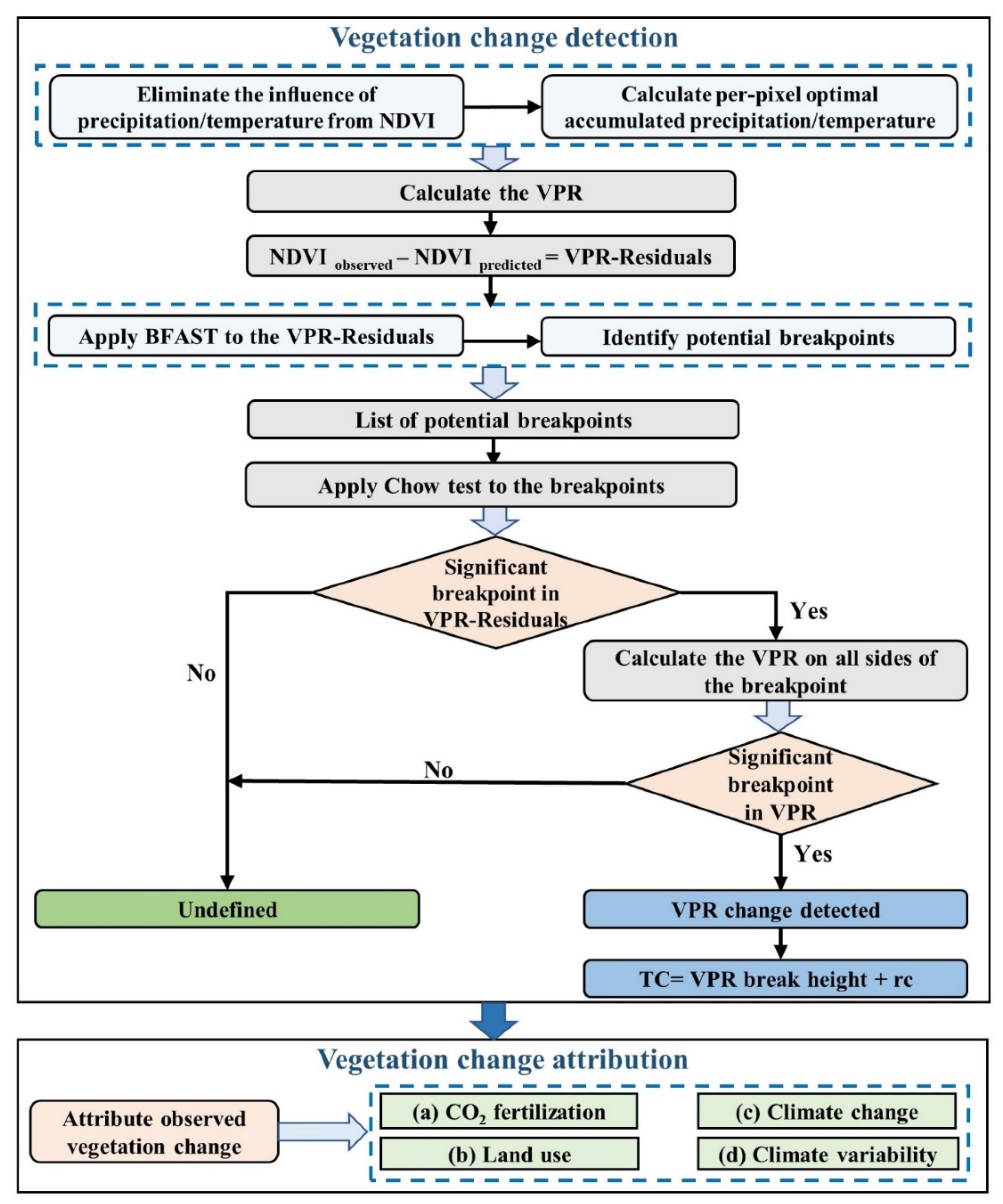
2.4. TSS-RESTREND Method

We performed the revised TSS-RESTREND v3.0 method to differentiate driving factors behind vegetation changes, including CO2, LU, CC, and CV. The TSS-RESTREND method includes two sections. The first used the complete NDVI time series to develop a list of potential breakpoints and assess the significance of these breakpoints and the second attributed the observed vegetation change. TSS-RESTREND can be sourced from an R package of ‘TSS.RESTREND’ (Available online: https://cran.r-project.org/web/packages/TSS.RESTREND/index.html accessed on 10 October 2020) [10]. The analysis procedure is illustrated in Figure 1:

2.4.1. The procedures of the TSS-RESTREND

The specific processing details of the method are summarized as follows:
  • Calculating the per-pixel optimal accumulated precipitation and temperature to eliminate the influence of precipitation and temperature from NDVI. They are obtained based on the optimal combination of the accumulation period (1–12 months) and offset period (0–4 months) with the annual peak growing season NDVI (NDVImax) [12]. In general, the peak growing season NDVI is equal to the annual max NDVI. The offset period describes the time between the end of the precipitation accumulation period and the occurrence of the NDVImax [26]. In this study, we defined the max accumulation period and offset period as 12 and 4 months, respectively.
  • Evaluating the vegetation-precipitation relationship (VPR) by calculating a pixel-based Ordinary Least Squares Regression between NDVImax and the optimal accumulated precipitation and temperature [27]. The VPR-Residuals were defined as the difference between the observed NDVI and NDVI predicted by the VPR at each period [12].

2.4.2. Breaks for Additive Seasonal and Trend and the Chow Test

Apply the Breaks for Additive Seasonal and Trend (BFAST) to the complete time-series VPR-Residuals to identify potential breakpoints [12,28]. The BFAST method is a widely used method for assessing variable trends in time series data in ecosystem assessment, which detects the phenological cycles that vegetation skipped without influencing ecological health as breakpoints [29]. A Chow test was used to check the breakpoints in VPR and residual trends, and then to assess whether these breakpoints have a significant impact [12,30]. The Chow test was applied to test the equality between coefficients in two linear regressions [30]. The null hypothesis of the Chow test is that no change exists in the regression coefficients across potential breakpoints. When the F-statistic reaches the critical threshold (α = 0.05), the null hypothesis is rejected [12].

2.4.3. Total Change and Attribution

If a significant breakpoint was detected in the VPR-Residuals, we then recalculate the VPR on all sides of the breakpoints and reapply a Chow test to assess the significance of these breakpoints in the VPR. Then, the total change (TC) of a pixel was calculated by adding the significant VPR break height to the residual change (rc) [12]. If no significant breakpoint was detected, the total change of vegetation was calculated by multiplying the observed trend by the length of the study period, and the magnitude of the trend was identified as significant when the p-value is less than 0.05.
Both precipitation and temperature data were used to attribute the observed vegetation change when using the TSSRattribution function in the R package of ‘TSS.RESTREND’, which requires both temperature and precipitation data to work. The observed vegetation change can be attributed to CO2, LU, CC, and CV. To differentiate the impacts of each contributor, we applied a 10-year moving window. We applied the method grid-by-grid at the global scale, and then visualized the results.

3. Results

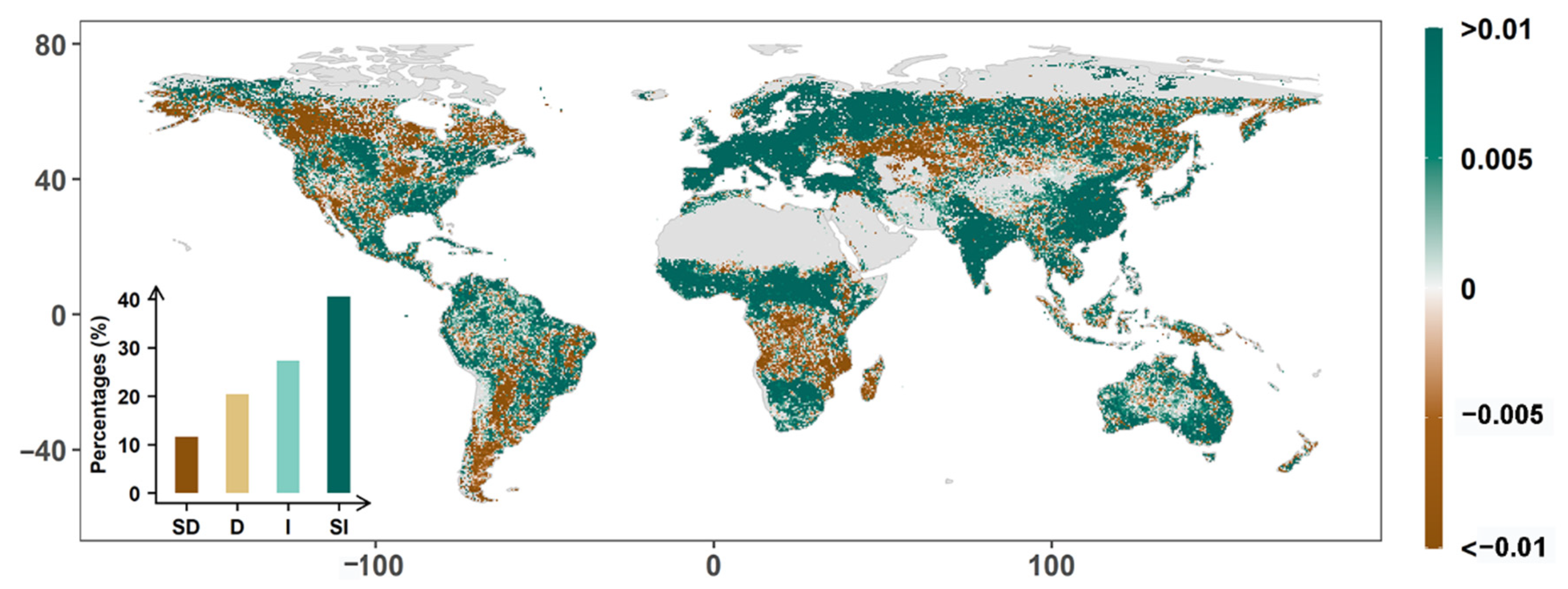
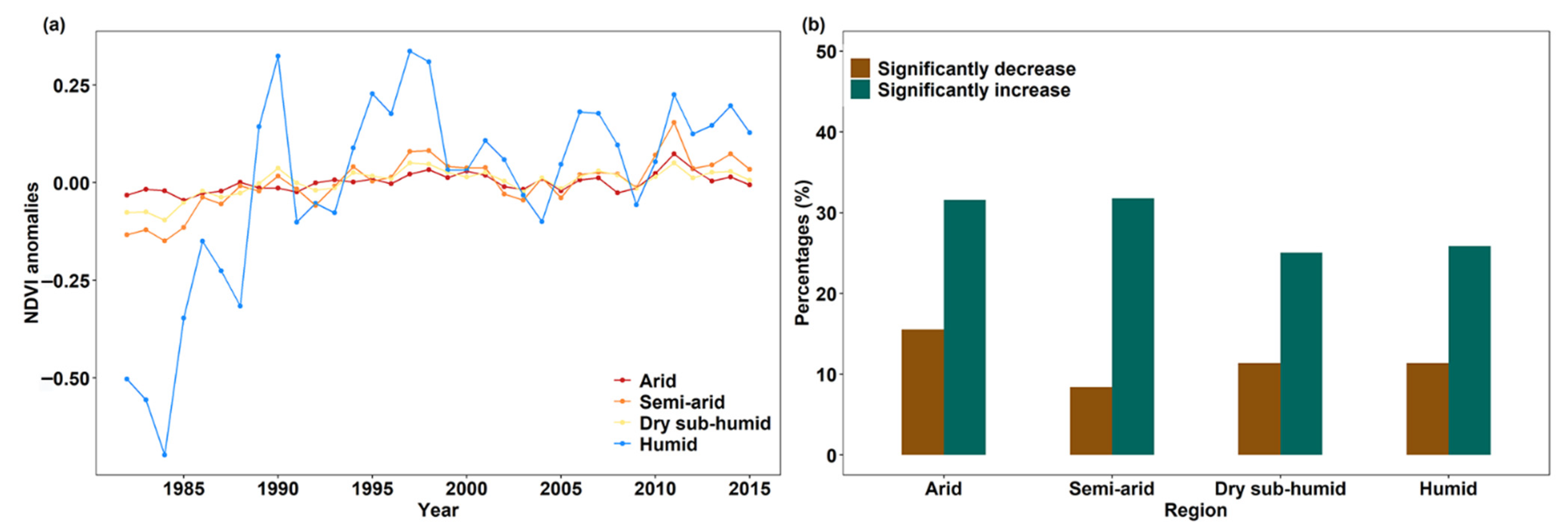
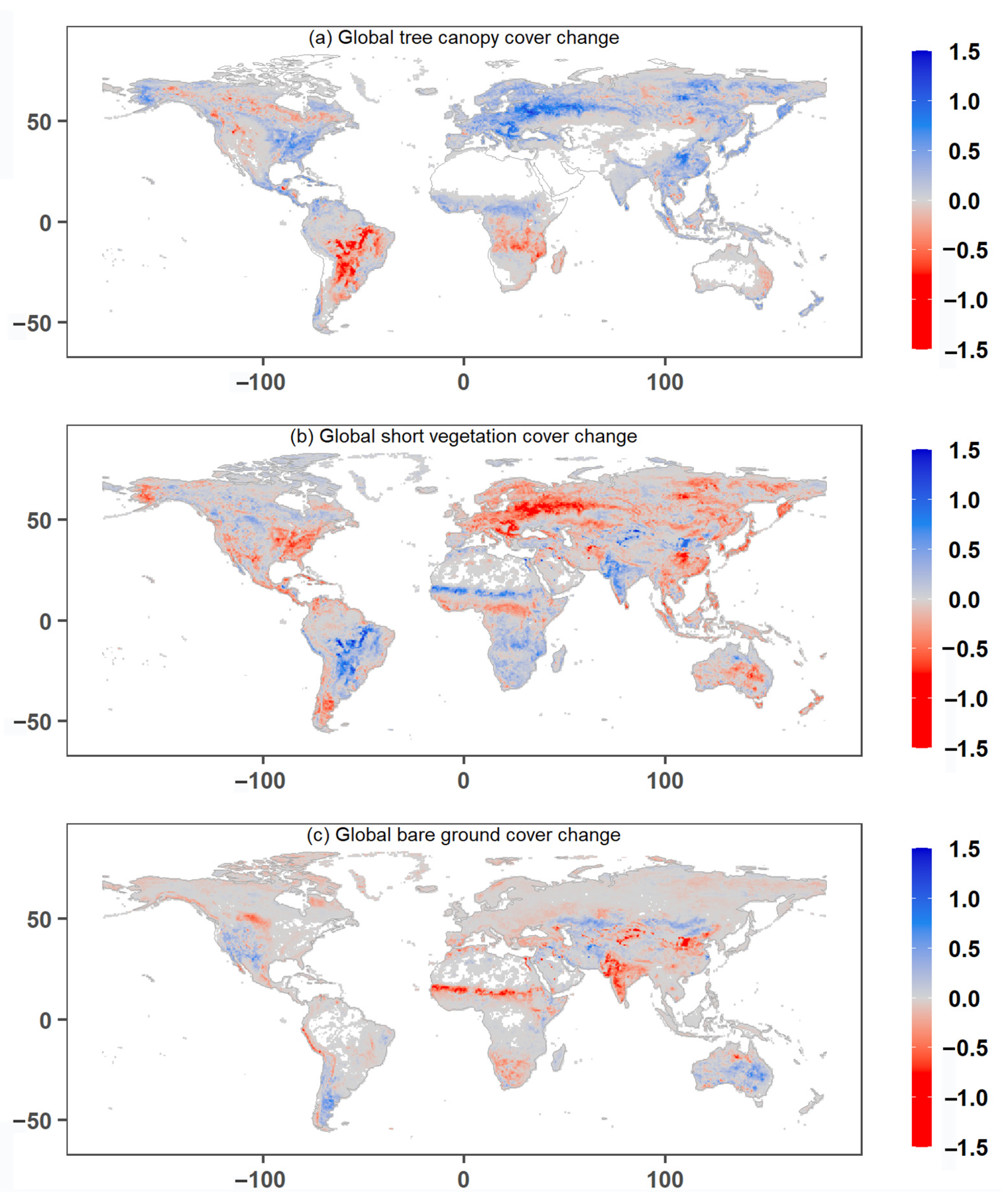
3.1. Global Greenness Changes from 1982–2015

The results of breakpoint detection indicate that there is no breakpoint in the global NDVI changes (Figures S4 and S5). Hence, we do not consider the breakpoint but calculate the vegetation dynamics using Sen’s slope estimator directly. The spatial pattern of trends in global annual NDVI from 1982 to 2015 indicates that 67.9% of global vegetated areas have seen an increase in annual NDVI since the 1980s (Figure 2), suggesting that widespread vegetation greening occurs globally. Overall, a significant increase in vegetation greenness is observed over 40.6% of the global vegetated grid cells. However, vegetation greenness changes vary considerably between regions. South Asia, Europe, East Asia, Sahel, and Australia are the regions with the most significant greening trends. In contrast, only 11.6% of the vegetated grid cells show significant decreasing trends (i.e., vegetation browning). The key places where vegetation is browning are central Asia, northern North America, southern South America, and central Africa. To figure out the regional vegetation change, we further examined the anomalies in NDVI for different dry and wet regions over the globe (Figure 3). NDVI anomalies represent the deviation of annual NDVI data from the multi-year average for each region. In general, NDVI values show an increasing trend during 1982–2015, but the interannual distribution of NDVI varied among different climatic zones. Specifically, the NDVI changes in arid, semi-arid, and dry sub-humid regions are relatively small, whereas NDVI changes in humid regions are noticeable with several mutation points (Figure 3a). In addition, we calculated the percentage of grids with a substantial change in NDVI to the total grids for each region (Figure 3b). Specifically, we notice that the regions with a high interannual variation in NDVI, such as in humid regions, do not necessarily have a significant upward trend. In other regions, however, the pattern was characterized by lower interannual variance but an upward trend in mean NDVI. We also found that the semi-arid regions are dominated by the most significant increase.

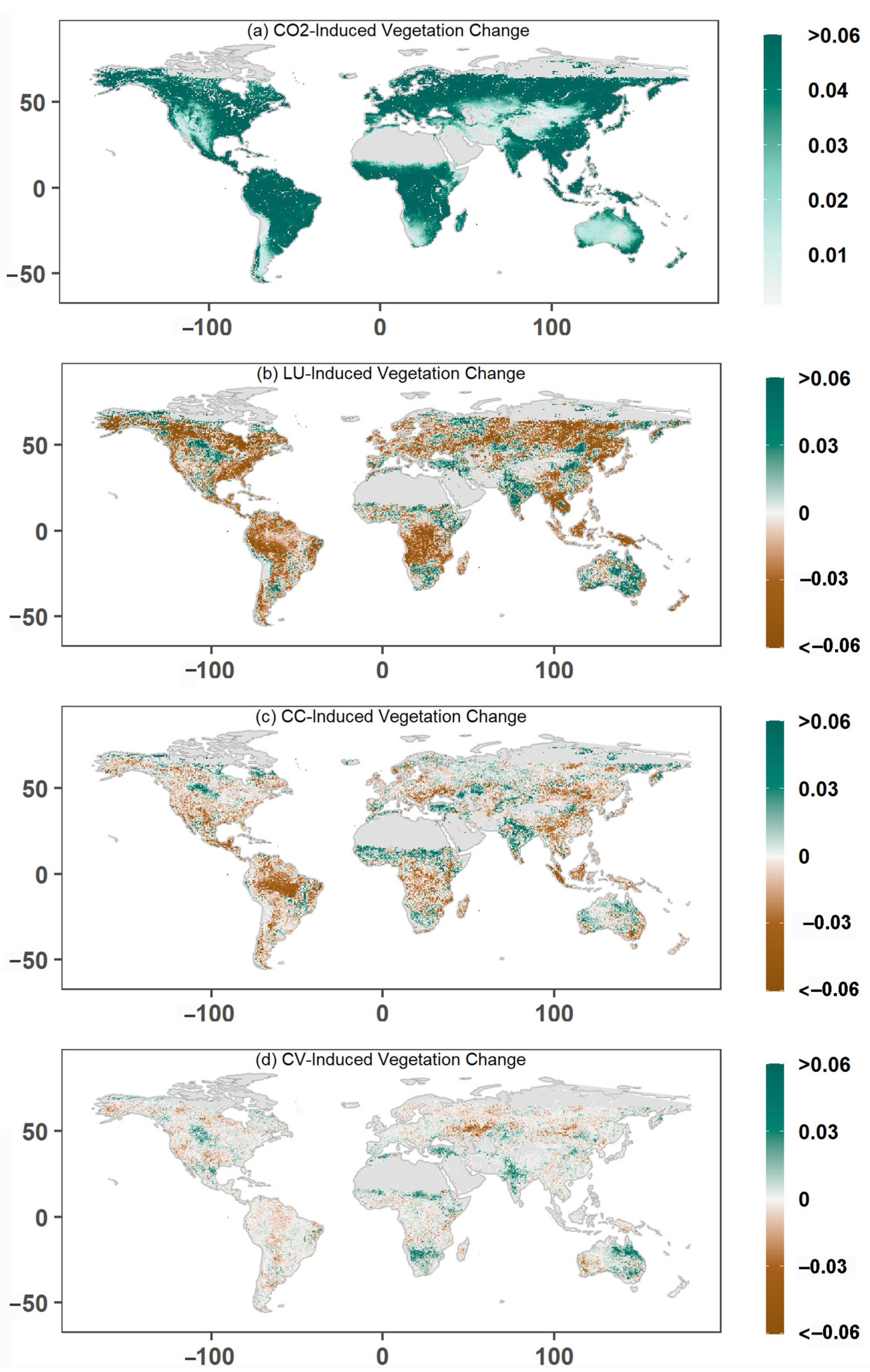
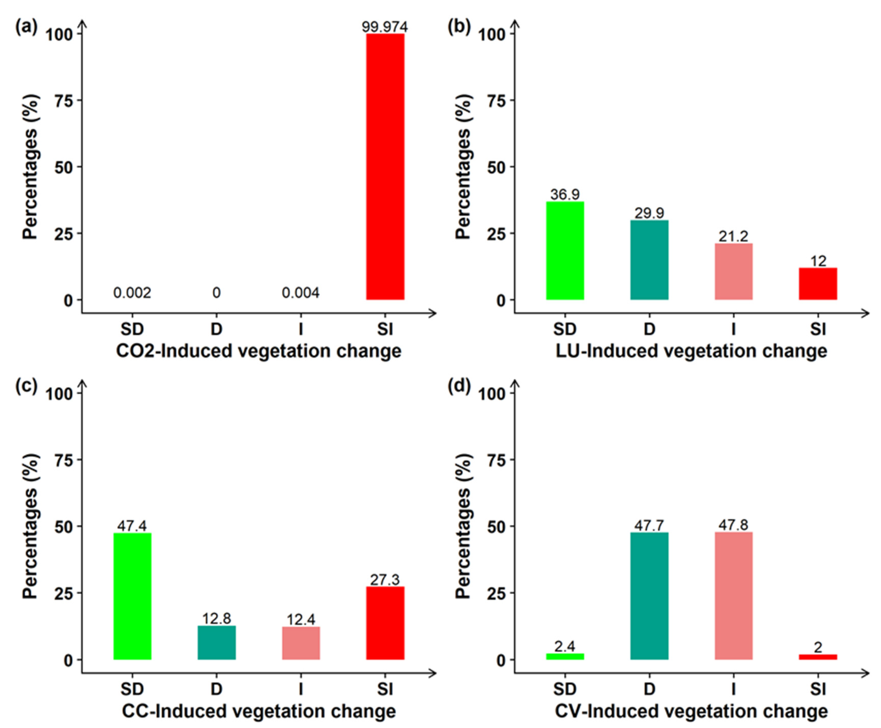
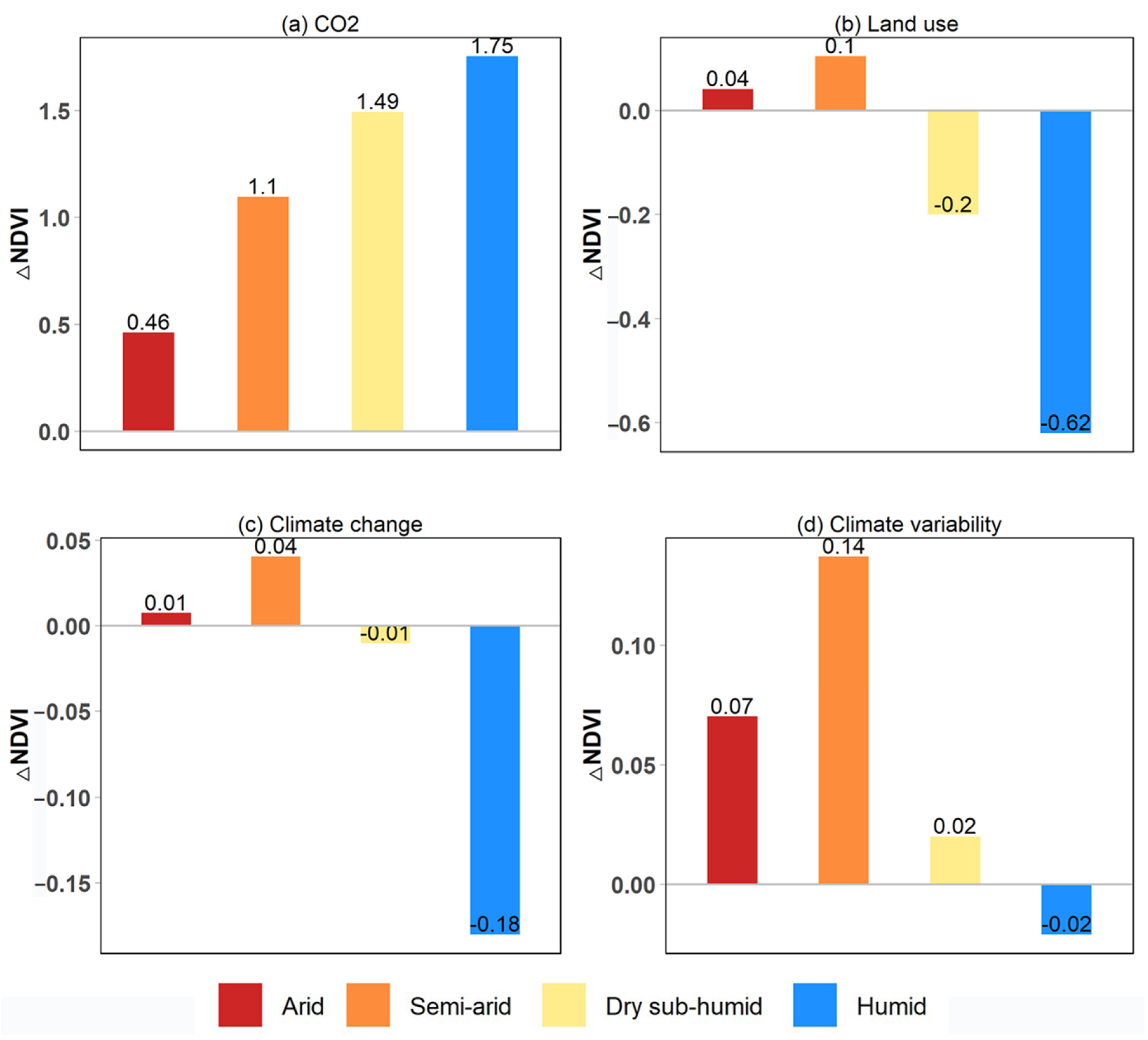
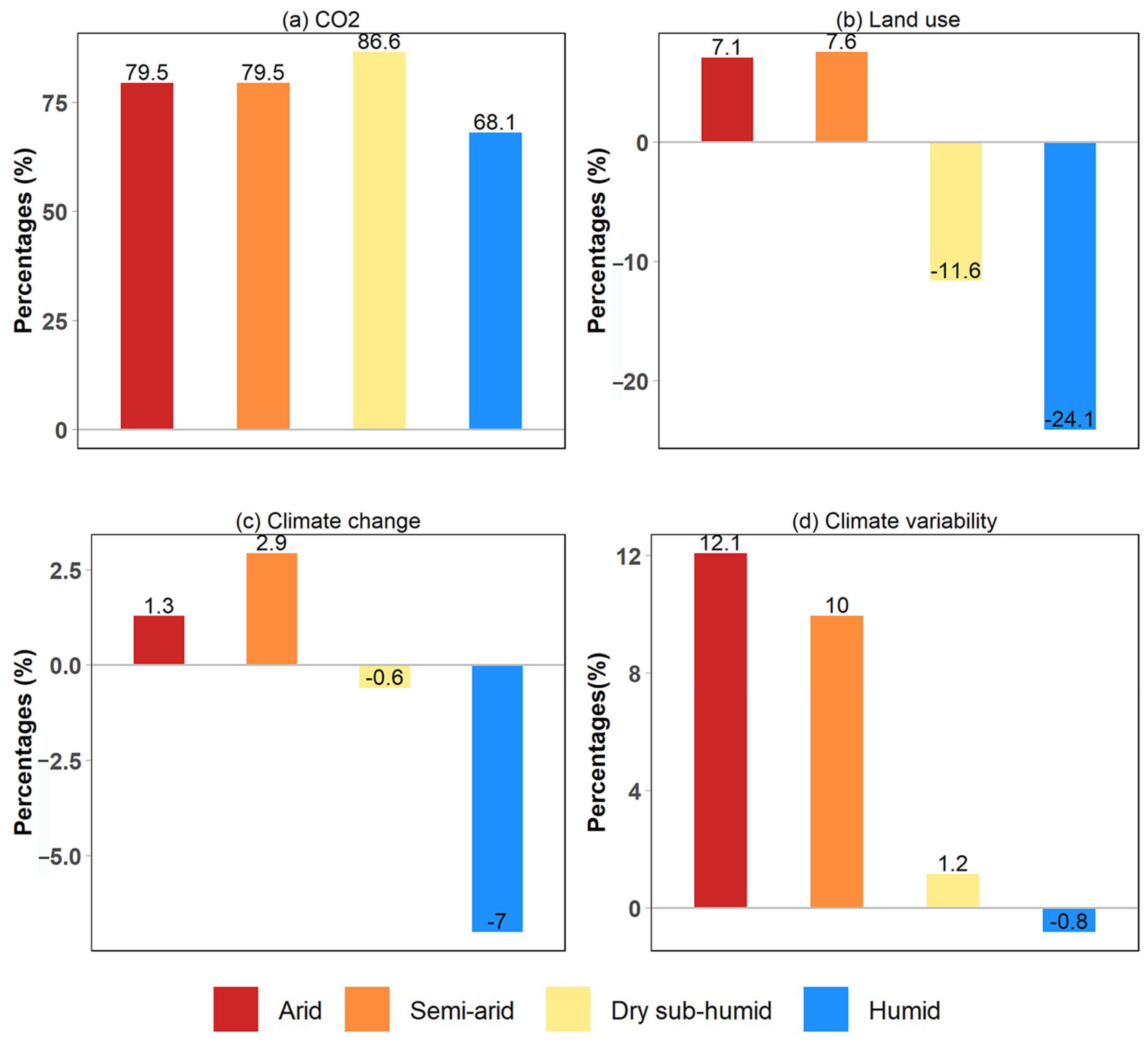
3.2. Drivers of Global Greening

We quantified the fractional contribution of CO2, LU, CC, and CV to the observed greening trends based on the TSS-RESTREND method (Figure 4).
CO2 positively impacts vegetation change (Figure 4a and Figure 5a), resulting in a 0.035 increase in global NDVI since the 1980s (Figure S6). Furthermore, CO2 has the largest absolute contribution to global vegetation greenness change in 61.4% of vegetated lands, followed by LU (23.5%), CC (7.3%), and then CV (1.5%) (Figure 6). To better understand the regional differences in the causes of vegetation change, we further investigated the impacts of four key driving factors on observed NDVI changes (ΔNDVI) in distinct dry and wet regions (Figure 7 and Figure S1). CO2 contributes most to the observed NDVI change in all regions, and its influence grows as humidity rises (Figure 7). In humid regions, CO2 fertilization has the smallest relative impact to observed NDVI change with a contribution of 68.1% (Figure 8).
LU negatively influenced global greening during 1982–2015, causing the global vegetation to change by −0.005 (Figure S6). The negative effects of LU can be found in 66.8% of global vegetated areas (Figure 5b). Hotspots, where LU has a negative impact, are Europe, northern Asia, central Africa, northern North America, and southern South America (Figure 4b). Furthermore, the impacts of LU have distinct dry-wet differences. Generally, LU reduces the vegetation greenness over dry sub-humid and humid regions by 11.6% and 24.1%, respectively (Figure 7b and Figure 8b). On the contrary, LU enhances the vegetation greenness in arid and semi-arid regions by an increase of 7.1% and 7.6%, respectively (Figure 7b and Figure 8b).
CC is thought to be an important driver of global greening. Overall, CC influences vegetation change across 7.3% of the global vegetated lands. Specifically, CC contributes the most to the vegetation greening across 2.8% of vegetated lands, whereas it dominates vegetation browning in 4.5% of vegetated lands (Figure 6). Besides, CC has significant positive impacts on vegetation greenness change across 27.3% of global vegetated areas, while the significant negative effects of CC on vegetation change are detected over 47.4% of the global vegetated areas (Figure 5c). The CC-related impacts on vegetation greenness are subject to evident regional heterogeneity, specifically, positive impacts in arid and semi-arid regions but negative impacts in dry sub-humid and humid regions. (Figure 7c and Figure 8c). Particularly, CC has distinct impacts on greenness change across humid areas, resulting in a 7% reduction in vegetation change in humid regions during 1982–2015 (Figure 8c).
Furthermore, the contribution of CV to global greenness change is also spatially heterogeneous. Specifically, CV has a fractional contribution of 12.1% and 10.0% to greenness in arid and semi-arid regions, respectively. However, its impacts are limited in the dry sub-humid and humid regions, which contribute just 1.2% and −0.8% to greenness change, respectively (Figure 7d and Figure 8d).

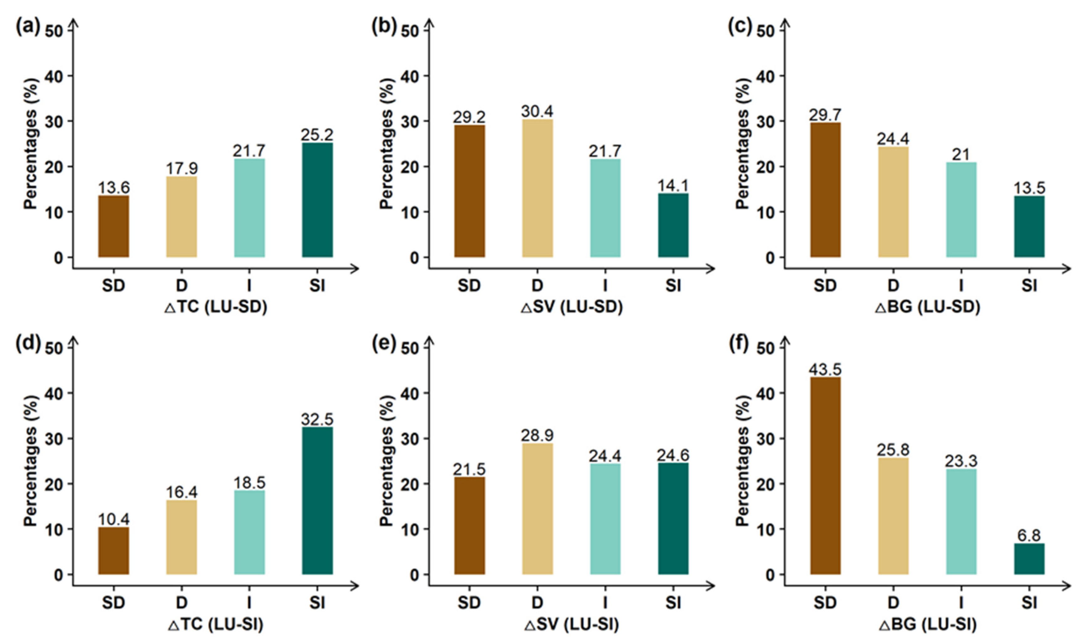
3.3. Impacts of Land Use Changes on Global Greening

LU, which has been continually modified by human activities, is intrinsically linked to the confluence of tree canopy (TC), short vegetation (SV), and bare ground (BG). We intercompared relative changes of global vegetated lands in eight sample regions with greening trends (Table 1). LU triggered increased greenness across densely-inhabited regions that underwent substantial LU activities during 1982–2015 (Figure 4b), such as the United States, Australia, China, and India. The increase of TC and the decrease of SV in the USA is a specific example (Figure 9a,b). In China, we observed obvious TC gain and SV loss (Figure 9a,b). We also found that cropland areas, agricultural land areas, and forest land areas in China have risen dramatically (Table 1). The greening of Australia can be partly attributed to human farming practices as cropland areas increased the most. In India, we saw considerable SV increase and BG loss (Figure 9b,c). The above-mentioned case studies imply that LU has discernable positive effects on observed greening. In recent years, we’ve also noticed vegetation browning over tropical regions (Figure 2). Specifically, the largest areas with net forest land loss are Brazil, Middle Africa, and Southern Africa during 1982–2015 (Table 1). Browning tendencies were discovered in Congo rainforests and South America, which can be attributed to LU (Figure 4b). Decreased TC cover is statistically significant over Congo rainforests. South America, being dominated by apparent TC loss, is characterized by a negative greening trend (Figure 9a). Simultaneously, some areas with decreasing SV show an increase in BG probably due to land degradation, resource exploitation, and urban sprawl [9]. The aforementioned results indicate constrained vegetation greening due to unsustainable LU activities.
Further highlighting the role of LU necessitates intercomparison between the proportion of areas with significant decrease, decrease, increase, and significant increase in different land cover types for the regions showing significant positive and negative impacts of LU on vegetation change (Figure 10). By increasing/decreasing the TC/BG cover, Positive LU (afforestation, irrigation, forestry, etc.) significantly affects the vegetation patterns. Specifically, for the regions with significant positive impacts of LU on vegetation change, 32.5% of regions show significant increasing trends of TC cover, while only 6.8% have significant growing trends of BG cover (Figure 10d–f). In contrast, we noticed that 13.5% of regions of BG cover show significant increasing trends when LU has significant negative impacts on regional vegetation change (Figure 10a–c).

4. Discussion

The dynamics of global vegetation have been experiencing substantial alterations due to ongoing climate change and human activities [3]. According to the findings of this study, a significant increase in global vegetation greenness was observed in 40.6% of the vegetated grid cells during 1982–2015, which is consistent with previous investigations [3,4]. Nevertheless, a study reported that global greenness change has been stagnating since 2000, because of the increased atmospheric vapor pressure deficit [31]. Contrary to this finding, a recent satellite data-based study found that around 33% of the global vegetated lands experienced greening while 5% experienced browning during 2000–2017 [5]. It’s possible that the reason why some previous studies reported the world stopped greening about 20 years ago may be an artifact of sensor degradation [32].
While model simulations almost show an increased global greening trend [3,4], there are, however, studies showing that some uncertainties actually exist in climate models in vegetation change detection [5]. We used the observation-based TSS-RESTREND v3.0 method to revisit the contribution of CO2, LU, CC, and CV on global vegetation change to further clarify this discussion on the dominant drivers of global greening. The analytical TSS-RESTREND method utilized herein has important implications for assessing and attributing changes in greenness caused by climate and land cover changes. Our findings revealed that CO2 fertilization was the dominant factor controlling vegetation changes, accounting for 61.4% of the global greening. Rising CO2 concentration in the atmosphere can enhance photosynthesis by accelerating the carboxylation rate [4,33]. Furthermore, increasing CO2 concentration can also strengthen the greenness of vegetation through processes including partially closing the leaf stomata [34]. We also found that CO2 was a key driver of the observed greening in arid and semi-arid areas, probably because CO2 has an impact on plant water savings and soil water increase [35].
Changes in LU markedly change the earth’s biogeochemical cycles, and further affect land surface properties [36]. A critical issue we concluded here was the strong relationship between vegetation browning and LU since LU has the largest absolute contribution to vegetation greenness decrease. Specifically, ecosystems that experience drought are more susceptible to showing a browning trend from LU, which is consistent with Webb et al. [37]. The browning of Congo rainforests, for instance, may relate to the deforestation caused by commodity crop cultivation [38]. The tropical deforestation caused by the expansion of the agricultural frontier probability results in the vegetation browning trend in South America [9]. According to a recent study, among the top ten countries/regions of the global largest karst ecosystems, Brazil was the only one exhibiting a larger extent of browning than greening, which nearly two-thirds can be ascribed to deforestation [39]. Chen et al. [5] reported the leading and impressive changes in agricultural production in Brazil with 25.6% of vegetated lands showing greening and 11.6% showing browning. However, the greening from croplands and pastures is nearly offset by the browning of forests [5,39]. Furthermore, the results showed that LU had a significant positive effect across 12% of global vegetated areas, especially in the United States of America, China, India, and Australia. The greening of the USA can be explained as forests recovering from historical interferences due to strengthened forestry management [40]. The implementation of afforestation initiatives was critical to the greening of northern and central China [5,10]. Changes in groundwater policy and improved irrigation practices leading to agricultural intensification may contribute to India’s increasing greenness [5]. The greening of Australia was driven by positive LU management, including agricultural intensification, and ecosystem recovery after the release of a viral biological control that killed 95% of Australia’s feral rabbits [12,41]. Overall, our findings provide agreements for a greater role of the human in global greening than previously thought.
The CC-induced greening may be largely related to the warming temperature since it can strengthen photosynthesis [3]. However, it should be pointed out that the positive impacts of CC on northern vegetation greenness change seem to be weak in recent years, which probably implies a saturation of future greenness change as the result of rising temperatures [42]. In water-limited ecosystems, precipitation change dominates the greenness change [43], as seen in the Sahel and southern Africa. Especially, we also noticed that the CC had significant negative impacts on vegetation change in South America. The CC-induced browning in South America can be explained as warming over these regions induced increased preseason precipitation and decreased growing season precipitation, and therefore led to drought stress [44]. Drought stress, in turn, counteracts early spring carbon assimilation and increases vegetation mortality [45].
The contribution of CV, which was not considered in previous studies, was found to have distinct impacts on the vegetated lands of arid regions, such as Sahel, India, and southern Africa. This phenomenon can be explained as vegetation in arid zones was more vulnerable to interferences from the external environment [11]. Our study highlights the indispensable role of CV on global greenness change. CV affects plant distribution as well as other plant characteristics, such as leaf transpiration, LAI, phenology, and net primary productivity (NPP) [46]. Because of the nonlinear interaction between climate systems and ecosystems, the mechanism of CV’s effects on plants is relatively complex, and is not fully understood. In the next step, we need to design a more reasonable experimental scheme, combined with the observation data, to do more in-depth research on the influence of CV on vegetation and its causes. In conclusion, these findings contribute to a better understanding of the underlying mechanisms of global greenness change and have important implications for vegetation change assessment and management.
Many studies have examined recent changes in vegetation growth and the associated climatic drivers, which revealed a global greening trend during the recent decades [3,4]. However, limited by modeling uncertainties [47], Chen et al. [5] pointed out that the models used in previous attribution analyses may underestimate the direct impacts of human activities on greening. Therefore, an observation-based attribution of the causes of the recent greening requires further investigation. A key benefit of this study is the opportunity to further investigate the role of human land use on global vegetation change by analyzing the trends in global land cover change for tree canopy, short vegetation, and bare ground. Furthermore, we intercompared relative changes of global vegetated lands in eight sample regions. In general, our observation-based results can improve our understanding of the underlying drivers of recent changes in global terrestrial vegetation activity. Besides, this study differs from the previous studies by making an extra step to examine the response of global vegetation change to the terms of internal climate variability. Furthermore, even though some studies reported the greening pattern at a global scale [3,4], the spatial patterns and temporal dynamics of vegetation greenness at the regional scale, as well as the reasons behind this, have rarely been investigated in the literature. The global vegetation-climate relationship is complex and has firm spatial heterogeneity [48]. Our regional assessment indicated that the impacts of LU and CC have distinct spatial heterogeneity, with positive impacts in arid regions but negative impacts in humid regions. Estimating the greening trend in dry-wet regions could help us understand the baseline vegetation dynamics under the ongoing climate changes, improving the reliability of future projected changes in vegetation [49].
Nonetheless, there are certain constraints ahead of us. Firstly, there exist some uncertainties in most products from satellite remote sensing, including but not limited to NDVI. For instance, the uncertainties of NDVI data are mainly derived from the loss of sensor calibration and orbital drift of satellites [4]. Secondly, the nonlinear relationship between vegetation changes and LU-related activities makes it difficult to separate the effect of specific LU activities on global vegetation change. We did not further quantify the contribution of specific LU activities on global greening in this study since long-term, large-scale observations of these factors are still lacking. Therefore, greater research into the precise role of LU is needed in the future to acquire a more comprehensive understanding of global greenness variations in a changing climate. Another limitation of our study is that we do not provide multiple tests of greenness detecting. A recent study reanalyzed global greening trends and advocated that part of the tested greening trends were false positives just because of the statistical testing mechanism [50].

5. Conclusions

Quantifying the causes of global greenness change has great significance to under-stand the process of vegetation dynamics and is the key for the prediction and management of global forest resources. Considering the critical shortcomings in previous model-based global assessments, this study performed an observation-based attribution of vegetation change across the globe. The global assessment shows a significant increase of vegetation greenness over 40.6% of the vegetated grid cells. However, only 11.6% of the vegetated grid cells show significant decreasing trends. Overall, global greening is mainly controlled by CO2 (61.4%), followed by LU (23.5%), CC (7.3%), and CV (1.5%).
The impacts of LU and CC have distinct spatial heterogeneity, that is, LU and CC have mainly positive impacts in arid and semi-arid regions while weakening the greenness in dry sub-humid and humid regions. The regions experiencing substantial LU activities, such as southeastern America, southeastern China, and India, show an increasing greening trend during 1982–2015. Positive LU practices affect the vegetation patterns by increasing the TC cover and decreasing the BG cover. We found that the tropical vegetation tended to undergo browning in recent years. The CV, an important driver ignored by previous research, was found to have a crucial impact on the vegetation change in arid and semi-arid regions, whereas it is limited in the dry sub-humid and humid regions. These results emphasize the indispensable impact of LU and CV in shaping the global vegetation change patterns.
Overall, our first observation-based attribution of vegetation change has important implications for understating the mechanism of global greening and supporting reliable future projections of vegetation changes. Continuing global vegetation change and the increasingly important role of LU and CC in modifying greenness patterns warrants continued and thorough investigation.

Supplementary Materials

The following supporting information can be downloaded at: https://www.mdpi.com/article/10.3390/rs14112706/s1, Figure S1: Global distribution of dry and wet regions; Figure S2: Global NDVI time series where the breakpoint is detected; Figure S3: Time series of the NDVI and precipitation for the period 1982–2015; Figure S4: The change in the vegetation-precipitation relationship (VPR); Figure S5: The segmented RESTREND applied using the segmented VPR; Figure S6: The mean contributions of driving factors on NDVI changes for the period 1982–2015.

Author Contributions

Conceptualization, J.L. and Q.Z.; methodology, C.L.; software, C.L.; validation, J.L. and Q.Z.; formal analysis, C.L. and J.L.; investigation, C.L.; resources, J.L.; data curation, C.L., J.L., and Q.Z.; writing—original draft preparation, C.L.; writing—review and editing, J.L., Q.Z., C.L., H.C., X.G., and A.G.; visualization, C.L.; supervision, J.L. and Q.Z.; project administration, J.L.; funding acquisition, J.L. All authors have read and agreed to the published version of the manuscript.

Funding

This research was funded by the National Natural Science Foundation of China (42001042), Opening funding of the State Key Laboratory of Hydrology-Water Resources and Hydraulic Engineering, Nanjing Hydraulic Research Institute (U2020nkms01), Visiting Researcher Fund Program of the State Key Laboratory of Water Resources and Hydropower Engineering Science (2020SWG02), Opening funding of the State Key Laboratory of Loess and Quaternary Geology, Institute of Earth Environment, CAS (SKLLQG2018), China Postdoctoral Science Foundation (BX20190301).

Data Availability Statement

The data are available from the website in the data section.

Acknowledgments

We appreciate Burrell, A.L. for providing the R package of ‘TSS.RESTREND’. We are grateful for the GIMMS3g NDVI and CRU meteorological dataset. We also thank Xihui Gu, Dongdong Kong, and Shuyun Feng for their kind comments and suggestions.

Conflicts of Interest

The authors declare no conflict of interest.

References

  1. Li, A.N.; Deng, W.; Liang, S.L.; Huang, C.Q. Investigation on the Patterns of Global Vegetation Change Using a Satellite-Sensed Vegetation Index. Remote Sens. 2010, 2, 1530–1548. [Google Scholar] [CrossRef] [Green Version]
  2. Walker, B.H. Landscape to regional-scale responses of terrestrial ecosystems to global change. Ambio 1994, 23, 67–73. [Google Scholar]
  3. Zhu, Z.C.; Piao, S.L.; Myneni, R.B.; Huang, M.T.; Zeng, Z.Z.; Canadell, J.G.; Ciais, P.; Sitch, S.; Friedlingstein, P.; Arneth, A.; et al. Greening of the Earth and its drivers. Nat. Clim. Chang. 2016, 6, 791–795. [Google Scholar] [CrossRef]
  4. Piao, S.L.; Wang, X.H.; Park, T.; Chen, C.; Lian, X.; He, Y.; Bjerke, J.W.; Chen, A.P.; Ciais, P.; Tommervik, H.; et al. Characteristics, drivers and feedbacks of global greening. Nat. Rev. Earth Environ. 2020, 1, 14–27. [Google Scholar] [CrossRef]
  5. Chen, C.; Park, T.; Wang, X.H.; Piao, S.L.; Xu, B.D.; Chaturvedi, R.K.; Fuchs, R.; Brovkin, V.; Ciais, P.; Fensholt, R.; et al. China and India lead in greening of the world through land-use management. Nat. Sustain. 2019, 2, 122–129. [Google Scholar] [CrossRef]
  6. Los, S.O. Analysis of trends in fused AVHRR and MODIS NDVI data for 1982-2006: Indication for a CO2 fertilization effect in global vegetation. Glob. Biogeochem. Cycles 2013, 27, 318–330. [Google Scholar] [CrossRef]
  7. Mao, J.F.; Ribes, A.; Yan, B.Y.; Shi, X.Y.; Thornton, P.E.; Seferian, R.; Ciais, P.; Myneni, R.B.; Douville, H.; Piao, S.L.; et al. Human-induced greening of the northern extratropical land surface. Nat. Clim. Chang. 2016, 6, 959–963. [Google Scholar] [CrossRef]
  8. Medlyn, B.E.; Zaehle, S.; De Kauwe, M.G.; Walker, A.P.; Dietze, M.C.; Hanson, P.J.; Hickler, T.; Jain, A.K.; Luo, Y.Q.; Parton, W.; et al. Using ecosystem experiments to improve vegetation models. Nat. Clim. Chang. 2015, 5, 528–534. [Google Scholar] [CrossRef]
  9. Song, X.P.; Hansen, M.C.; Stehman, S.V.; Potapov, P.V.; Tyukavina, A.; Vermote, E.F.; Townshend, J.R. Global land change from 1982 to 2016. Nature 2018, 560, 639–643. [Google Scholar] [CrossRef]
  10. Burrell, A.L.; Evans, J.P.; De Kauwe, M.G. Anthropogenic climate change has driven over 5 million km2 of drylands towards desertification. Nat. Commun. 2020, 11, 3853. [Google Scholar] [CrossRef]
  11. Chen, C.; He, B.; Yuan, W.P.; Guo, L.L.; Zhang, Y.F. Increasing interannual variability of global vegetation greenness. Environ. Res. Lett. 2019, 14, 12. [Google Scholar] [CrossRef]
  12. Burrell, A.L.; Evans, J.P.; Liu, Y. Detecting dryland degradation using Time Series Segmentation and Residual Trend analysis (TSS-RESTREND). Remote Sens. Environ. 2017, 197, 43–57. [Google Scholar] [CrossRef]
  13. Liu, C.X.; Melack, J.; Tian, Y.; Huang, H.B.; Jiang, J.X.; Fu, X.; Zhang, Z.A. Detecting Land Degradation in Eastern China Grasslands with Time Series Segmentation and Residual Trend analysis (TSS-RESTREND) and GIMMS NDVI3g Data. Remote Sens. 2019, 11, 1014. [Google Scholar] [CrossRef] [Green Version]
  14. Ruan, Z.; Kuang, Y.Q.; He, Y.Y.; Zhen, W.; Ding, S. Detecting Vegetation Change in the Pearl River Delta Region Based on Time Series Segmentation and Residual Trend Analysis (TSS-RESTREND) and MODIS NDVI. Remote Sens. 2020, 12, 4049. [Google Scholar] [CrossRef]
  15. Li, Z.D.; Wang, S.; Song, S.; Wang, Y.P.; Musakwa, W. Detecting land degradation in Southern Africa using Time Series Segment and Residual Trend (TSS-RESTREND). J. Arid Environ. 2021, 184, 9. [Google Scholar] [CrossRef]
  16. Pinzon, J.E.; Tucker, C.J. A Non-Stationary 1981–2012 AVHRR NDVI3g Time Series. Remote Sens. 2014, 6, 6929–6960. [Google Scholar] [CrossRef] [Green Version]
  17. Hashimoto, H.; Wang, W.L.; Dungan, J.L.; Li, S.; Michaelis, A.R.; Takenaka, H.; Higuchi, A.; Myneni, R.B.; Nemani, R.R. New generation geostationary satellite observations support seasonality in greenness of the Amazon evergreen forests. Nat. Commun. 2021, 12, 684. [Google Scholar] [CrossRef]
  18. Peng, S.S.; Piao, S.L.; Ciais, P.; Myneni, R.B.; Chen, A.P.; Chevallier, F.; Dolman, A.J.; Janssens, I.A.; Penuelas, J.; Zhang, G.X.; et al. Asymmetric effects of daytime and night-time warming on Northern Hemisphere vegetation. Nature 2013, 501, 88–94. [Google Scholar] [CrossRef]
  19. Harris, I.; Osborn, T.J.; Jones, P.; Lister, D. Version 4 of the CRU TS monthly high-resolution gridded multivariate climate dataset. Sci. Data 2020, 7, 109. [Google Scholar] [CrossRef] [Green Version]
  20. Wang, B.; Xu, G.C.; Li, P.; Li, Z.B.; Zhang, Y.X.; Cheng, Y.T.; Jia, L.; Zhang, J.X. Vegetation dynamics and their relationships with climatic factors in the Qinling Mountains of China. Ecol. Indic. 2020, 108, 105719. [Google Scholar] [CrossRef]
  21. Murphy, B.F.; Timbal, B. A review of recent climate variability and climate change in southeastern Australia. Int. J. Climatol. 2008, 28, 859–879. [Google Scholar] [CrossRef]
  22. Gao, X.J.; Giorgi, F. Increased aridity in the Mediterranean region under greenhouse gas forcing estimated from high resolution simulations with a regional climate model. Glob. Planet. Chang. 2008, 62, 195–209. [Google Scholar] [CrossRef]
  23. Meinshausen, M.; Smith, S.J.; Calvin, K.; Daniel, J.S.; Kainuma, M.L.T.; Lamarque, J.F.; Matsumoto, K.; Montzka, S.A.; Raper, S.C.B.; Riahi, K.; et al. The RCP greenhouse gas concentrations and their extensions from 1765 to 2300. Clim. Chang. 2011, 109, 213–241. [Google Scholar] [CrossRef] [Green Version]
  24. FAO. FAOSTAT Database; FAO: Rome, Italy, 2018. [Google Scholar]
  25. Hansen, M.C.; Defries, R.S.; Townshend, J.R.G.; Sohlberg, R. Global land cover classification at 1 km spatial resolution using a classification tree approach. Int. J. Remote Sens. 2000, 21, 1331–1364. [Google Scholar] [CrossRef]
  26. Evans, J.; Geerken, R. Discrimination between climate and human-induced dryland degradation. J. Arid. Environ. 2004, 57, 535–554. [Google Scholar] [CrossRef]
  27. Wessels, K.J.; van den Bergh, F.; Scholes, R.J. Limits to detectability of land degradation by trend analysis of vegetation index data. Remote Sens. Environ. 2012, 125, 10–22. [Google Scholar] [CrossRef]
  28. Verbesselt, J.; Hyndman, R.; Newnham, G.; Culvenor, D. Detecting trend and seasonal changes in satellite image time series. Remote Sens. Environ. 2010, 114, 106–115. [Google Scholar] [CrossRef]
  29. Broich, M.; Huete, A.; Tulbure, M.G.; Ma, X.; Xin, Q.; Paget, M.; Restrepo-Coupe, N.; Davies, K.; Devadas, R.; Held, A. Land surface phenological response to decadal climate variability across Australia using satellite remote sensing. Biogeosciences 2014, 11, 5181–5198. [Google Scholar] [CrossRef] [Green Version]
  30. Chow, G.C. Tests of equality between sets of coefficients in two linear regressions. Econometrica 1960, 28, 591–605. [Google Scholar] [CrossRef]
  31. Yuan, W.P.; Zheng, Y.; Piao, S.L.; Ciais, P.; Lombardozzi, D.; Wang, Y.P.; Ryu, Y.; Chen, G.X.; Dong, W.J.; Hu, Z.M.; et al. Increased atmospheric vapor pressure deficit reduces global vegetation growth. Sci. Adv. 2019, 5, 12. [Google Scholar] [CrossRef] [Green Version]
  32. Zhang, Y.L.; Song, C.H.; Band, L.E.; Sun, G.; Li, J.X. Reanalysis of global terrestrial vegetation trends from MODIS products: Browning or greening? Remote Sens. Environ. 2017, 191, 145–155. [Google Scholar] [CrossRef] [Green Version]
  33. Farquhar, G.D.; Sharkey, T.D. Stomatal conductance and photosynthesis. Annu. Rev. Plant Physiol. Plant Mol. Biol. 1982, 33, 317–345. [Google Scholar] [CrossRef]
  34. Keenan, T.F.; Hollinger, D.Y.; Bohrer, G.; Dragoni, D.; Munger, J.W.; Schmid, H.P.; Richardson, A.D. Increase in forest water-use efficiency as atmospheric carbon dioxide concentrations rise. Nature 2013, 499, 324–327. [Google Scholar] [CrossRef]
  35. Lu, X.F.; Wang, L.X.; McCabe, M.F. Elevated CO2 as a driver of global dryland greening. Sci. Rep. 2016, 6, 7. [Google Scholar] [CrossRef] [Green Version]
  36. Foley, J.A.; DeFries, R.; Asner, G.P.; Barford, C.; Bonan, G.; Carpenter, S.R.; Chapin, F.S.; Coe, M.T.; Daily, G.C.; Gibbs, H.K.; et al. Global consequences of land use. Science 2005, 309, 570–574. [Google Scholar] [CrossRef] [PubMed] [Green Version]
  37. Webb, N.P.; Marshall, N.A.; Stringer, L.C.; Reed, M.S.; Chappell, A.; Herrick, J.E. Land degradation and climate change: Building climate resilience in agriculture. Front. Ecol. Environ. 2017, 15, 450–459. [Google Scholar] [CrossRef]
  38. Ordway, E.M.; Asner, G.P.; Lambin, E.F. Deforestation risk due to commodity crop expansion in sub-Saharan Africa. Environ. Res. Lett. 2017, 12, 13. [Google Scholar] [CrossRef]
  39. Tang, X.G.; Xiao, J.F.; Ma, M.G.; Yang, H.; Li, X.; Ding, Z.; Yu, P.J.; Zhang, Y.G.; Wu, C.Y.; Huang, J.; et al. Satellite evidence for China’s leading role in restoring vegetation productivity over global karst ecosystems. For. Ecol. Manag. 2022, 507, 120000. [Google Scholar] [CrossRef]
  40. Birdsey, R.; Pregitzer, K.; Lucier, A. Forest carbon management in the United States: 1600-2100. J. Environ. Qual. 2006, 35, 1461–1469. [Google Scholar] [CrossRef] [PubMed] [Green Version]
  41. Schwensow, N.I.; Cooke, B.; Kovaliski, J.; Sinclair, R.; Peacock, D.; Fickel, J.; Sommer, S. Rabbit haemorrhagic disease: Virus persistence and adaptation in Australia. Evol. Appl. 2014, 7, 1056–1067. [Google Scholar] [CrossRef]
  42. Piao, S.L.; Nan, H.J.; Huntingford, C.; Ciais, P.; Friedlingstein, P.; Sitch, S.; Peng, S.S.; Ahlstrom, A.; Canadell, J.G.; Cong, N.; et al. Evidence for a weakening relationship between interannual temperature variability and northern vegetation activity. Nat. Commun. 2014, 5, 7. [Google Scholar] [CrossRef] [Green Version]
  43. Fensholt, R.; Langanke, T.; Rasmussen, K.; Reenberg, A.; Prince, S.D.; Tucker, C.; Scholes, R.J.; Le, Q.B.; Bondeau, A.; Eastman, R.; et al. Greenness in semi-arid areas across the globe 1981–2007—An Earth Observing Satellite based analysis of trends and drivers. Remote Sens. Environ. 2012, 121, 144–158. [Google Scholar] [CrossRef]
  44. Teng, H.F.; Luo, Z.K.; Chang, J.F.; Shi, Z.; Chen, S.C.; Zhou, Y.; Ciais, P.; Tian, H.Q. Climate change-induced greening on the Tibetan Plateau modulated by mountainous characteristics. Environ. Res. Lett. 2021, 16, 11. [Google Scholar] [CrossRef]
  45. Angert, A.; Biraud, S.; Bonfils, C.; Henning, C.C.; Buermann, W.; Pinzon, J.; Tucker, C.J.; Fung, I. Drier summers cancel out the CO2 uptake enhancement induced by warmer springs. Proc. Natl. Acad. Sci. USA 2005, 102, 10823–10827. [Google Scholar] [CrossRef] [Green Version]
  46. Zeng, X.D. Evaluating the dependence of vegetation on climate in an improved dynamic global vegetation model. Adv. Atmos. Sci. 2010, 27, 977–991. [Google Scholar] [CrossRef]
  47. Zhao, L.; Dai, A.G.; Dong, B. Changes in global vegetation activity and its driving factors during 1982–2013. Agric. For. Meteorol. 2018, 249, 198–209. [Google Scholar] [CrossRef]
  48. Myers-Smith, I.H.; Kerby, J.T.; Phoenix, G.K.; Bjerke, J.W.; Epstein, H.E.; Assmann, J.J.; John, C.; Andreu-Hayles, L.; Angers-Blondin, S.; Beck, P.S.A.; et al. Complexity revealed in the greening of the Arctic. Nat. Clim. Chang. 2020, 10, 106–117. [Google Scholar] [CrossRef] [Green Version]
  49. Qiao, N.; Wang, L.X. Satellite observed vegetation dynamics and drivers in the Namib sand sea over the recent 20 years. Ecohydrology 2022, 15, e2420. [Google Scholar] [CrossRef]
  50. Cortes, J.; Mahecha, M.D.; Reichstein, M.; Myneni, R.B.; Chen, C.; Brenning, A. Where Are Global Vegetation Greening and Browning Trends Significant? Geophys. Res. Lett. 2021, 48, e2020GL091496. [Google Scholar] [CrossRef]
Figure 1. Flowchart of TSS-RESTREND method.
Remotesensing 14 02706 g001
Figure 2. Trends in annual GIMMS NDVI during 1982–2015. The grey color represents the barren areas. Antarctica and Greenland have been removed from the data. The inset histogram shows the percentages of grids showing significant decrease (SD), decrease (D), increase (I), and significant increase (SI).
Remotesensing 14 02706 g002
Figure 3. Vegetation changes for different dry-wet regions. (a) The interannual variations and (b) the percentage of grids showing significant changes in NDVI for different dry and wet regions during 1982–2015.
Remotesensing 14 02706 g003
Figure 4. Driving factors of global vegetation change. The NDVI changes during 1982–2015 were attributed to (a) CO2 fertilization (CO2), (b) land use (LU), (c) climate change (CC), and (d) climate variability (CV).
Remotesensing 14 02706 g004
Figure 5. Percentages of grids with trends in a significant decrease (SD), decrease (D), increase (I), and significant increase (SI) caused by (a) CO2 fertilization (CO2), (b) land use (LU), (c) climate change (CC), and (d) climate variability (CV).
Remotesensing 14 02706 g005
Figure 6. The dominant contributor of NDVI changes. The driving factors include CO2 fertilization (CO2), land use (LU), climate change (CC), and climate variability (CV), as well as the residual (Res). The prefix ‘+’ means a positive impact on NDVI trends, while ‘−’ means a negative impact. The inset shows the percentage of areas dominated by each contributor.
Remotesensing 14 02706 g006
Figure 7. The impacts of (a) CO2 fertilization (CO2), (b) land use (LU), (c) climate change (CC), and (d) climate variability (CV) on observed NDVI changes (ΔNDVI) in different dry and wet regions during 1982–2015.
Remotesensing 14 02706 g007
Figure 8. The relative contribution rate of (a) CO2 fertilization (CO2), (b) land use (LU), (c) climate change (CC), and (d) climate variability (CV) to the observed NDVI changes in different dry and wet regions during 1982–2015.
Remotesensing 14 02706 g008
Figure 9. The trends in global land cover change for (a) tree canopy (TC), (b) short vegetation (SV), and (c) bare ground (BG) during 1982–2015.
Remotesensing 14 02706 g009
Figure 10. The roles of special land cover types in the effects of land use (LU) on vegetation change. The percentage of areas with significant decrease (SD), decrease (D), increase (I), and significant increase (SI) in different land cover types for the regions showing significant (ac) negative and (df) positive impacts of land use on vegetation change. TC, SV, and BG represent the areas covered by tree canopy, short vegetation, and bare ground, respectively.
Remotesensing 14 02706 g010
Table 1. Global land-cover area changes during 1982–2015. Limited by the observation, the forest land change is calculated by using the data covering 1990–2015.
RegionsForest Land
(×103 ha)
Agricultural Land (×103 ha)Cropland
(×103 ha)
Arable Land
(×103 ha)
The globe−147,724 (−3.5%)87,933 (1.9%)118,397 (8.3%)50,145 (3.8%)
Australia−788 (−0.6%)−142,653 (−29.1%)11,784 (60.1%)11,648 (59.9%)
Brazil−85,013 (−14.4%)−872 (−0.4%)3051 (5.1%)4978 (10.0%)
China53,154 (33.8%)85,215 (19.2%)29,900 (28.2%)17,143 (16.7%)
European Union28,335 (21.3%)−16,077 (−8.1%)−7727 (−6.1%)−6343 (−5.6%)
India6890 (10.8%)−1097 (−0.6%)670 (0.4%)−6830 (−4.2%)
Middle Africa−34,001 (−10.3%)4319 (2.7%)10,940 (44.7%)10,200 (47.7%)
Northern America6487 (1.0%)−29,900 (−6.1%)−32,864 (−14.2%)−33,617 (−14.7%)
Southern Africa−5612 (−12.1%)2183 (1.3%)−254 (−1.8%)−382 (−2.8%)
Publisher’s Note: MDPI stays neutral with regard to jurisdictional claims in published maps and institutional affiliations.

