Tradeoffs between UAS Spatial Resolution and Accuracy for Deep Learning Semantic Segmentation Applied to Wetland Vegetation Species Mapping

Abstract

Recent advances in image classification of fine spatial resolution imagery from unoccupied aircraft systems (UASs) have allowed for mapping vegetation based on both multispectral reflectance and fine textural details. Convolutional neural network (CNN)-based models can take advantage of the spatial detail present in UAS imagery by implicitly learning shapes and textures associated with classes to produce highly accurate maps. However, the spatial resolution of UAS data is infrequently examined in CNN classification, and there are important tradeoffs between spatial resolution and classification accuracy. To improve the understanding of the relationship between spatial resolution and classification accuracy for a CNN-based model, we captured 7.6 cm imagery with a UAS in a wetland environment containing graminoid (grass-like) plant species and simulated a range of spatial resolutions up to 76.0 cm. We evaluated two methods for the simulation of coarser spatial resolution imagery, averaging before and after orthomosaic stitching, and then trained and applied a U-Net CNN model for each resolution and method. We found untuned overall accuracies exceeding 70% at the finest spatial resolutions, but classification accuracy decreased as spatial resolution coarsened, particularly beyond a 22.8 cm resolution. Coarsening the spatial resolution from 7.6 cm to 22.8 cm could permit a ninefold increase in survey area, with only a moderate reduction in classification accuracy. This study provides insight into the impact of the spatial resolution on deep learning semantic segmentation performance and information that can potentially be useful for optimizing precise UAS-based mapping projects.

1. Introduction

Unoccupied aircraft systems (UASs) with fine spatial resolution (centimeter-scale) sensors have opened the door to new capabilities in the field of remote sensing [1]. Furthermore, known as unoccupied aerial vehicles (UAVs) or drones, these systems typically capture images with spatial resolutions in the centimeter range, small enough to measure fine-scale land surface texture and spectral reflectance. Highly detailed analyses, such as species-level vegetation classification, are possible at these resolutions [1]. For a given sensor, lower flight altitudes produce images with a higher spatial resolution, while reducing the spatial extent captured by a single image. This tradeoff is of critical importance for classifying land cover from UAS data—spatial resolution must be sufficiently fine to produce high classification accuracy, but spatial coverage must be sufficiently extensive to map the area of concern. It is possible to increase coverage by planning many flights, although at the expense of time and equipment cost, and longer duration acquisition campaigns can introduce issues with illumination conditions caused by solar zenith angle and cloud cover. Therefore, it is crucial to consider this tradeoff and the best UAS flight parameters for an application.

In the early history of remote sensing land cover classification, Markham and Townshend [2] described the relationship between classification accuracy and sensor spatial resolution. The authors documented the impact of boundary pixels—the pixels that form a transition between land cover classes—as one of the causes of reduced classification accuracy at a coarser spatial resolution. Larger pixels are likely to encompass several land cover types; these pixels are referred to as mixed pixels. The thematic precision of the classification scheme used to map land cover (e.g., ecosystem type, lifeform, or individual species for vegetation) is also dependent on the spatial resolution [3]. In vegetated ecosystems where texture provides important information for distinguishing classes, less precise classification schemes (e.g., ecosystem type) can be mapped using coarser spatial resolution data, whereas more precise classification schemes (e.g., individual species) require finer spatial resolution data.

Alongside the proliferation of UAS remote sensing in recent years, there have been significant developments in algorithms for classifying fine spatial resolution imagery. Deep learning techniques, especially convolutional neural network (CNN)-based models, have been frequently applied in recent literature [4]. An advantage of CNNs is that they utilize the spatial detail contained within imagery to learn textures, shapes, and edges and make land cover predictions through the application of pixel convolutions. CNNs incorporate context through their ‘sliding window’ nature; classes are identified as a kernel passes through the image, as opposed to operating on a single pixel like a multilayer perceptron. Advanced deep learning models integrate several convolution layers and include techniques specifically designed to deal with fine details, such as Cheng et al. [5], who produced a new discriminative objective function for training models.

CNNs have proven particularly useful for fine-scale mapping of invasive species from UAS data [6,7,8,9,10]. Detecting invasive species using remote sensing benefits from the use of high spatial resolution image data that enable the precise mapping of invasives at incipient levels and provide for targeted management strategies. In addition, the use of a UAS allows for repeat, opportunistic monitoring of invasions at a scale that would be much more costly and time-consuming using ground surveys alone. Recent examples of CNN-based models applied to UAS data for invasive species mapping includes trees [7,11], reeds [10], and several herbaceous species [6,8,9]. The ability of CNNs to take advantage of vegetation texture fits well with the fine spatial resolution provided by UAS imagery; however, the tradeoffs between spatial resolution and CNN classification accuracy are not well quantified.

In a review of CNNs in vegetation remote sensing, Kattenborn et al. [12] found recent studies that have compared classification accuracies at very fine spatial resolutions [13,14,15]. These studies compared resolutions from 0.3 to 32 cm and found substantial reductions in classification performance as the spatial resolution was coarsened. However, these studies mapped large plants (trees and banana plants) in forest or farm ecosystems, hence the need for a more in-depth analysis of spatial resolution’s impact on CNN classification accuracy for smaller-leaved graminoid (grass-like) plants in a wetland environment. Only Schiefer et al. [15] implemented a semantic segmentation model but did not explicitly test the effects of different approaches for simulating coarser resolution imagery on model accuracy.

The objective of this research is to investigate changes in CNN classification accuracy for mapping wetland graminoid species with changes in spatial resolution to better understand the tradeoffs between spatial resolution and classification accuracy for UAS image acquisition campaigns. This research uses data acquired in a wetland habitat dominated by three graminoid species that share similarities in appearance but have differing canopy structures. While the focus of this study is on one particular environment, changes in CNN accuracy with coarsening resolution can provide insight into the loss of spatial detail that can occur in other vegetation types and reveal tradeoffs between spatial resolution and accuracy.

2. Materials and Methods

2.1. Study Area and Data

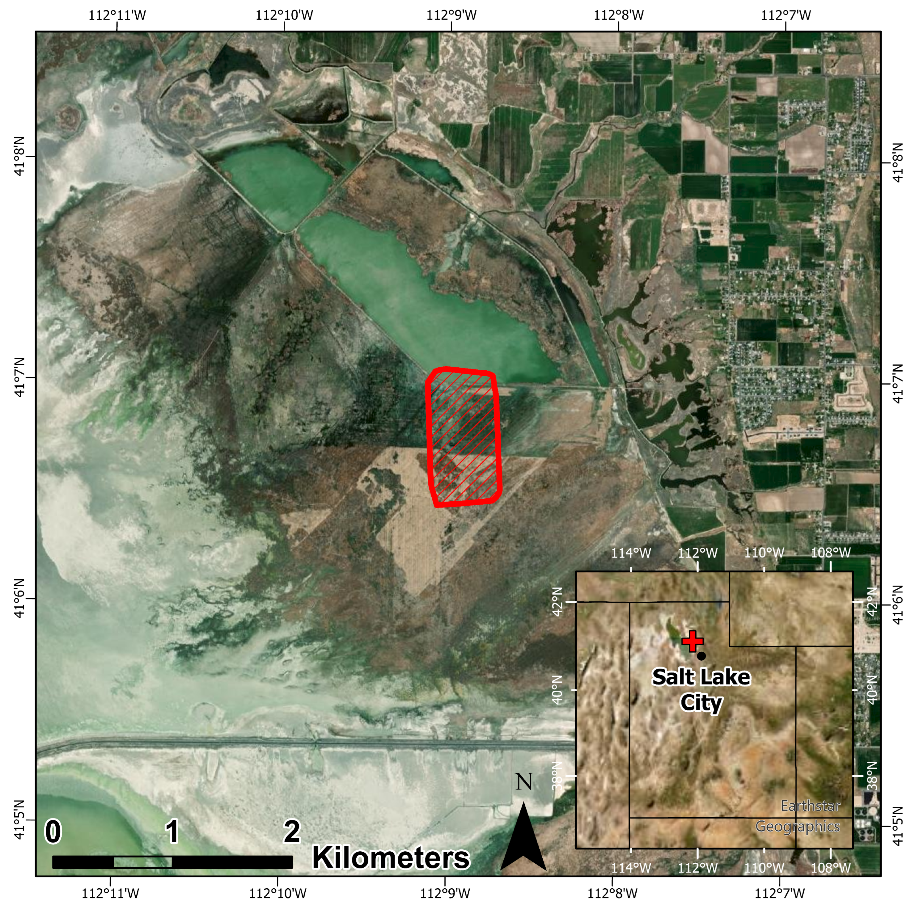
The study area was in the Howard Slough Waterfowl Management Area, approximately 45 km northwest of Salt Lake City, Utah, USA (Figure 1). The habitat was a marshy wetland with permanently wet or intermittently flooded areas that can be difficult to access on foot. Water levels depend on the season, recent weather events, and manual flood management. 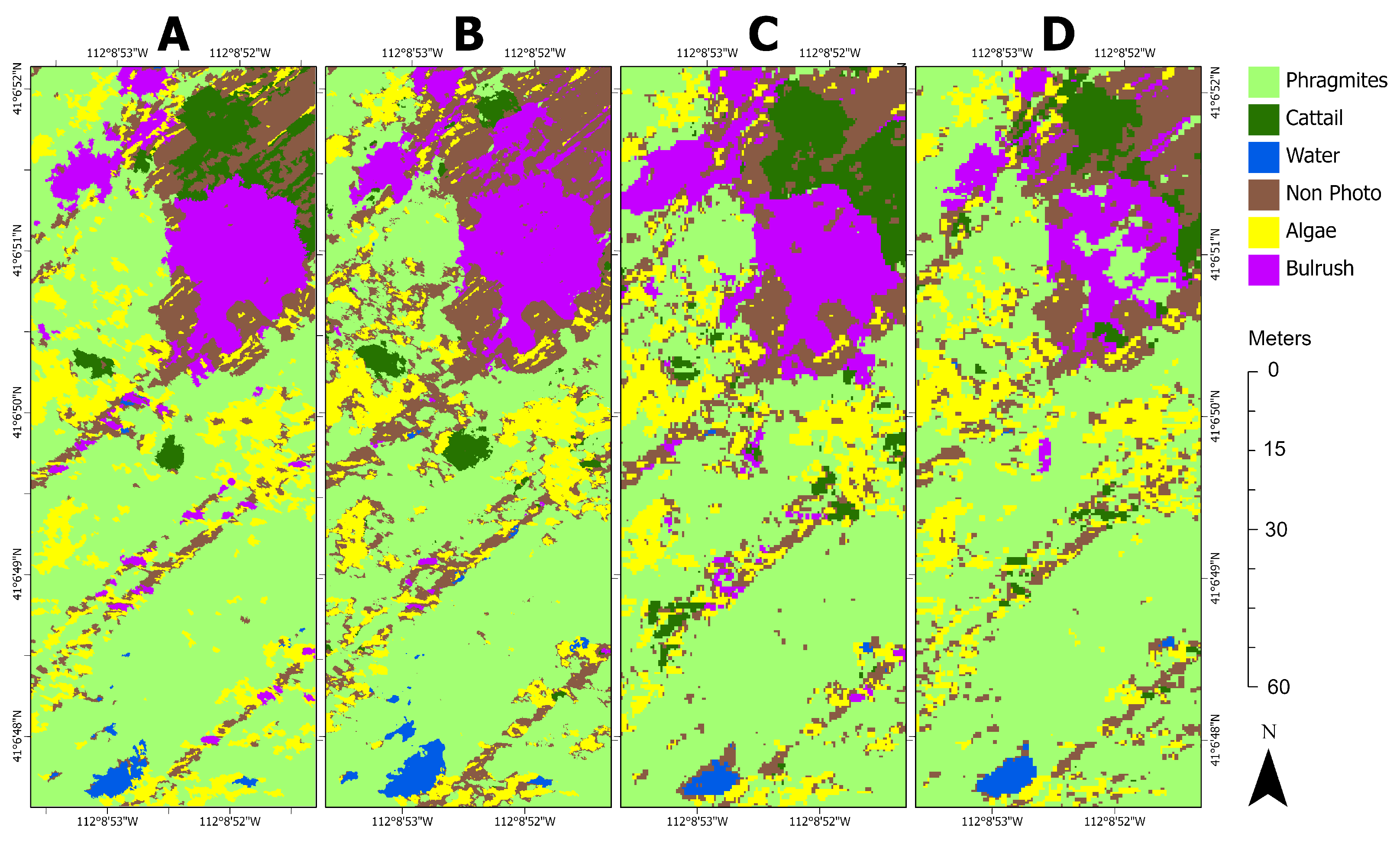Vascular plant cover at the site was dominated by three herbaceous vegetation types: the invasive common reed (Phragmites australis), native cattail (Typha latifolia), and bulrushes (Schoenoplectus americanus, Schoenoplectus acutus). Additional land cover types included water, non-photosynthetic vegetation, and algae (Figure 2). There was very little elevation change at the site, and it was at about 1280 m in elevation.

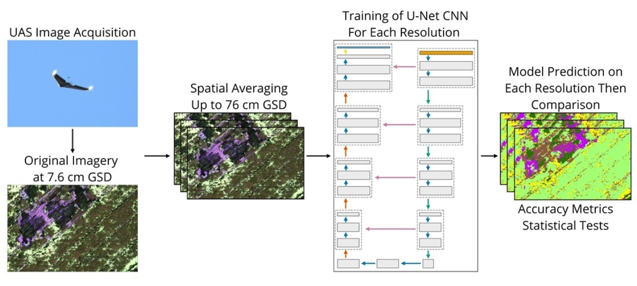
The images analyzed in this study were acquired in August 2020. A Parrot Disco fixed-wing UAS (Paris, France) was modified to house a MicaSense RedEdge-MX sensor (Seattle, WA, USA). This sensor measured five spectral bands: blue, green, red, red edge, and near infrared (

Table 1. RedEdge-MX sensor bands.

Band	Blue	Green	Red	Red Edge	Near Infrared
Band Center	475 nm	560 nm	668 nm	717 nm	840 nm
Bandwidth	32 nm	27 nm	16 nm	12 nm	57 nm

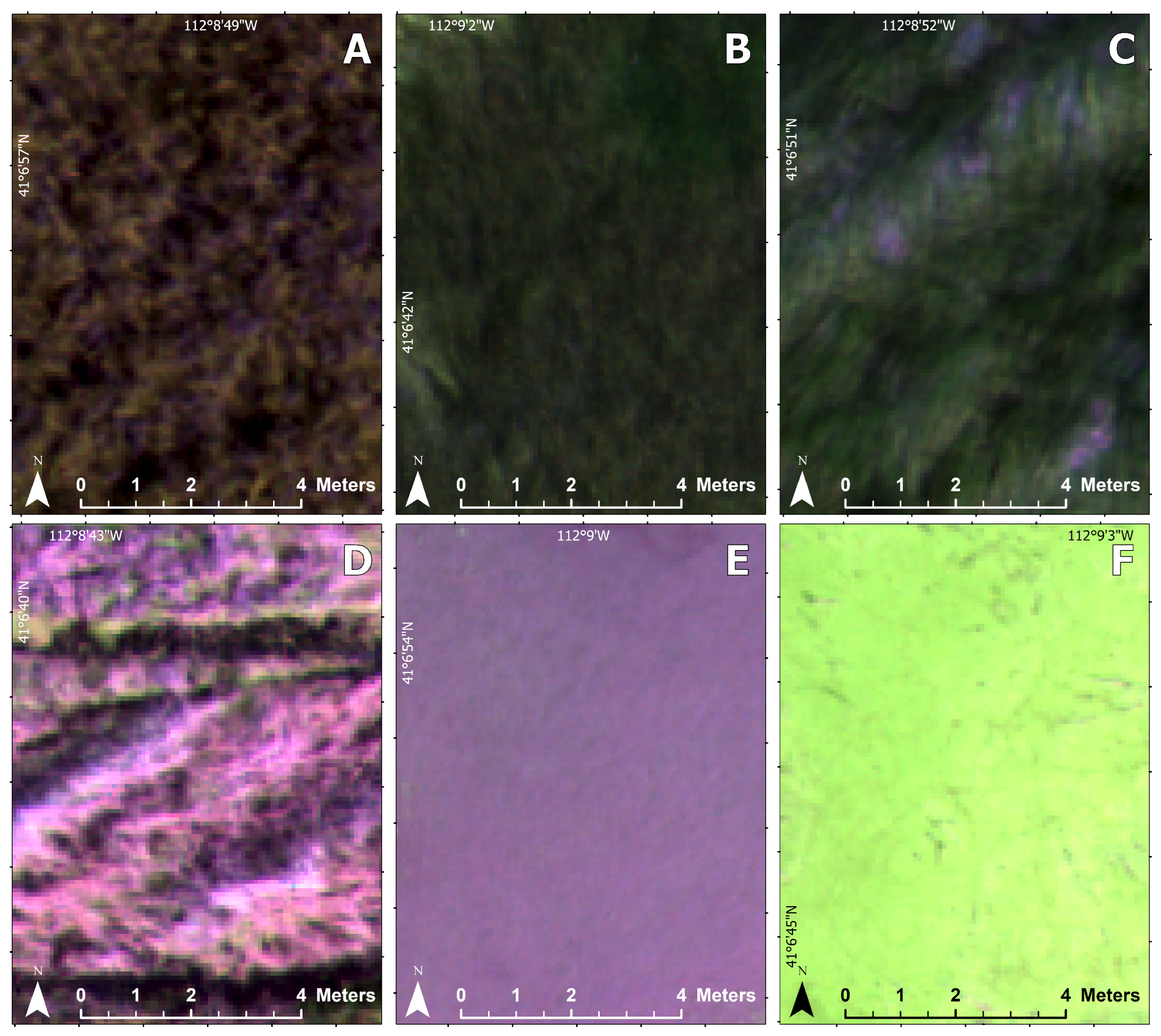
). The data were processed in Pix4D (Prilly, Switzerland), which stitched the imagery together using image overlap to produce a color-balanced orthomosaic. The image dimensions were approximately 8000 pixels × 15,000 pixels × 5 bands with a 7.6 cm spatial resolution in the 16-bit TIFF image format. The orthomosaic covered approximately 60 hectares. Figure 3 shows an example of each land cover class in the orthomosaic.

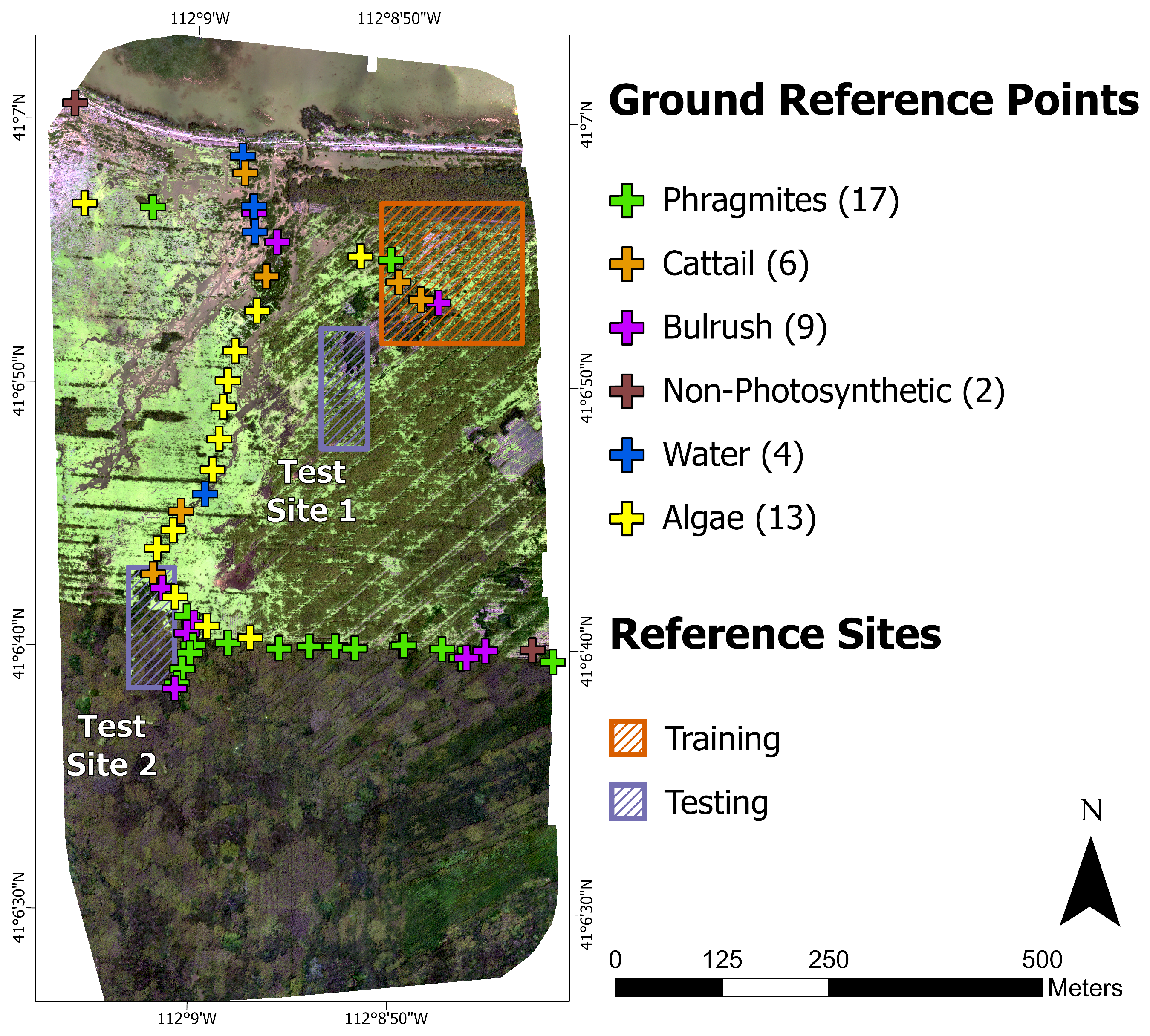
Ground reference data were collected in late July 2020. Reference data were collected opportunistically due to the difficulty of traversing the wetland landscape. Fifty-two points were captured in ArcGIS QuickCapture with a GPS-enabled smartphone (5 m accuracy) by the Utah Department of Natural Resources’ invasive species coordinator and labeled as belonging to one of the six classes (Figure 2). Each point represents a circular area of at least 1 m², and photos (with camera pointing direction) were taken at each point (Figure 4). There is active management of the invasive Phragmites at the site involving the operation of an amphibious vehicle, resulting in a ‘striped’ appearance of vegetation in the imagery where the vehicle traveled.

2.2. Image Processing

Images with a range of spatial resolutions over the same area can be created through two methods: independent data acquisitions or simulation. Independent data acquisitions require multiple flights at different altitudes over the same study area. Lighting conditions change throughout the day, as well as weather conditions and potentially vegetation conditions over several days. Additionally, georeferencing errors between the flights can influence the accuracy assessment. The simulation method only requires a single capture and post-processing to resample the imagery to coarser resolutions, reducing the number of uncontrolled variables.

A detector’s instantaneous field of view (IFOV) and the instrument flight altitude determine a pixel’s spatial resolution [16]. The area measured on the surface—referred to as the ground instantaneous field of view (GIFOV)—does not equally contribute to the reflected solar radiance measured by the detector; the area near the center of the GIFOV is more heavily weighted, and areas outside of a square pixel can also be within the GIFOV [17,18]. The point spread function (PSF) describing the weighting of the area measured within the GIFOV is unique to the instrument’s optics, the detector and electronics, atmospheric effects, and any resampling used on measurements [17]. While the simulation method can explicitly account for the sensor’s PSF, a spatial averaging approach is typically used to simulate coarser resolution imagery [19,20,21] and can closely approximate resampling by incorporating a sensor’s PSF [22]. Spatial averaging is an unweighted average of the original pixels onto a coarser resolution grid, where a pixel at ½ resolution (‘2× resample factor’) would be computed by the average value of the nearest four original pixels.

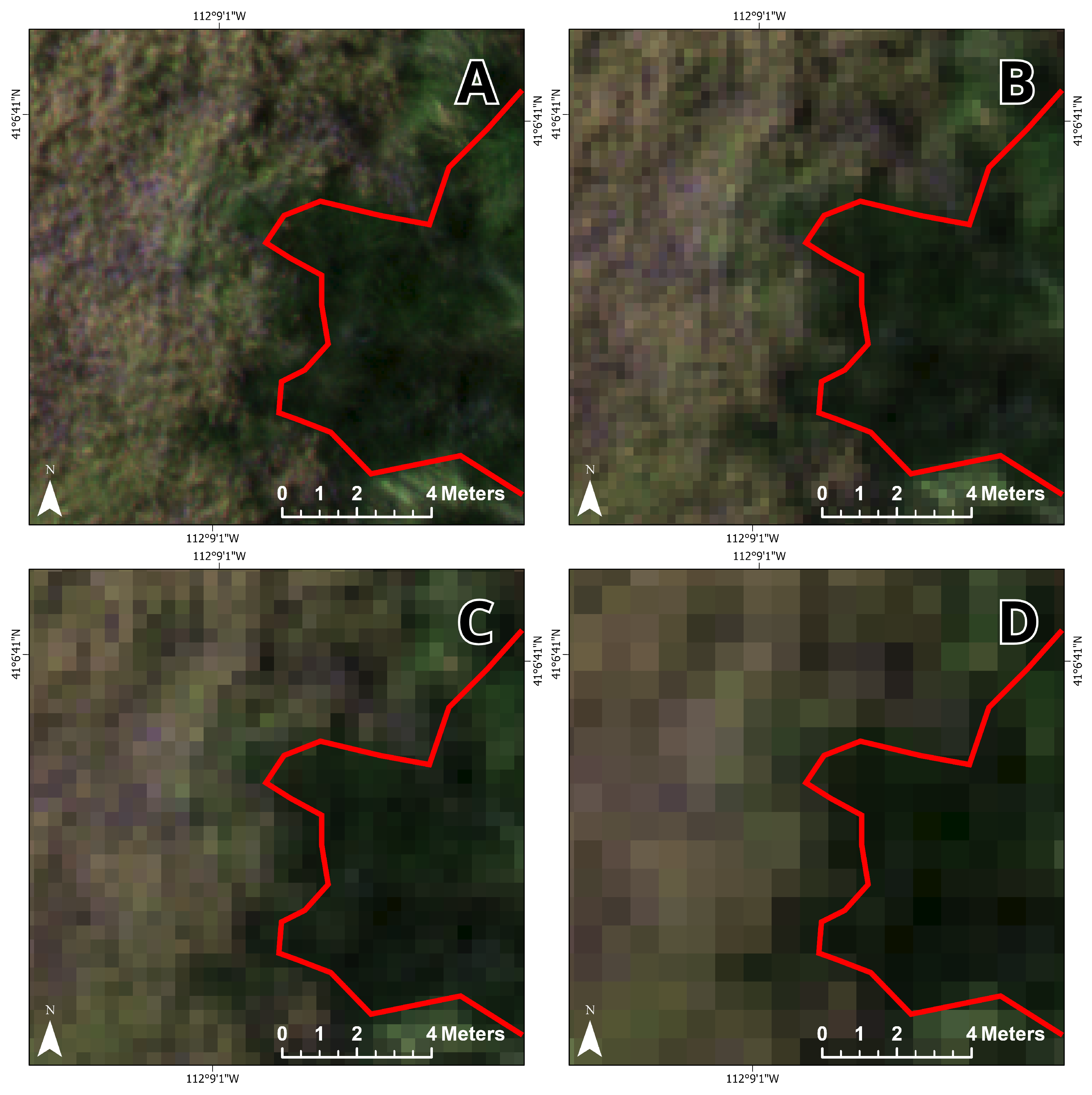
Two different approaches were taken for spatial averaging of the UAS image data: (1) the before orthomosaic resampling (BOR) method and (2) the after orthomosaic resampling (AOR) method. For the BOR method, spatial averaging was performed per each RedEdge-MX band before image mosaicking and orthorectification in Pix4D to simulate a range of spatial resolutions. The BOR method was applied to coarser spatial resolutions until orthorectification metrics exceeded thresholds for assessing the output quality. The AOR method averaged pixels after orthorectification and was applied across a wider range of spatial resolutions. This comparison was undertaken because BOR was believed to more accurately represent the process of mosaicking images captured at varying spatial resolutions, either by using a lower-resolution sensor or by flying at a higher altitude, but can only be simulated over a narrow range of resolutions due to limitations in mosaicking images with relatively few pixels. In contrast, AOR enables analysis across a broader range of spatial resolutions but does not independently mosaic each spatial resolution.

Pix4D processing parameters include image width and height, camera focal length, principal point image coordinates, and radial and tangential distortion factors. Pix4D has a database for common sensors such as the RedEdge-MX, and the original resolution imagery was processed using the parameters from the database. For the spatially averaged imagery, the image width and height, focal length, and principal point image coordinates were downscaled proportionately to the image resolution. The radial and tangential distortion factors were not varied, as these distortions are due to the camera’s lenses [23] and remain spatially consistent through resampling. Once processing was completed, Pix4D computed a quality report (

Table 2. Image stitching report from Pix4D for original resolution and spatially aggregated imagery using the before orthomosaic resampling (BOR) method.

Resample Factor	Resolution (cm)	Keypoints (Median)	Calibration (%)	Optimization (%)	Matching (Median)
Original	7.6	10,000	95	0.05	3479
2×	15.2	8622	96	0.26	3288
3×	22.8	3863	96	0.82	1919
4×	30.4	2188	95	0.30	1196
5×	38.0	1410	95	2.02	820

). The number of keypoints, or distinct points in the image, represents the amount of visual content in the image that can be used for matching between overlapping images for stitching. The calibration percentage indicates the number of images that share a sufficient number of keypoints with other images and can be reliably stitched. The optimization percentage specifies the deviation from the input parameters (e.g., scene center coordinates) after Pix4D tunes the parameters. Matching is the median number of matching keypoints between images, indicating the reliability of the results. Beyond a 5× coarsening in spatial resolution (from 7.6 cm to 38.0 cm), the quality report showed that the results were no longer reliable; the median number of keypoints dropped below 1000, the calibration was below 95%, optimization above 5%, and the median number of matches were below 500.

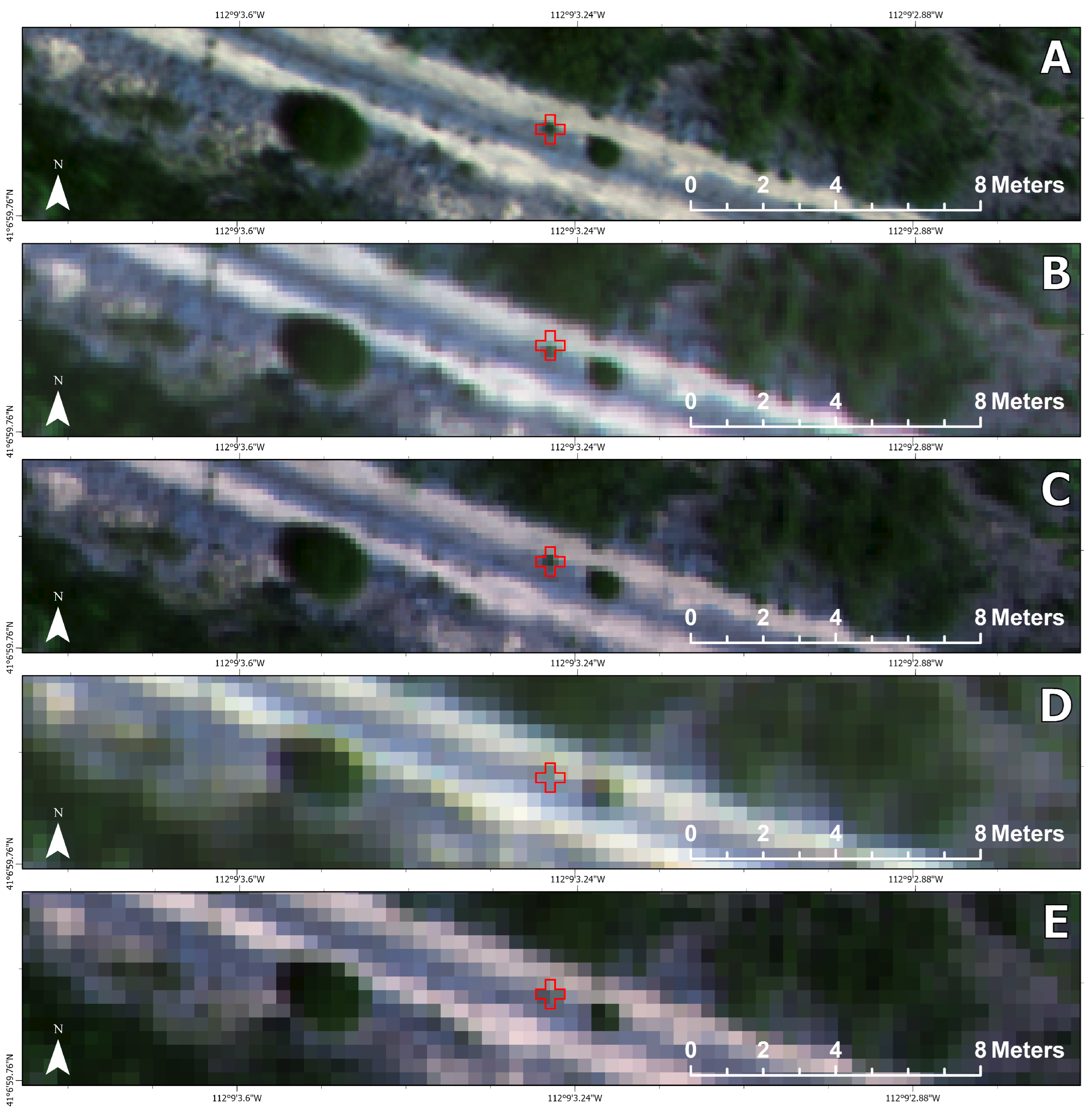
For the AOR method, the 7.6 cm orthomosaic was spatially degraded with average resampling to between 2× (15.2 cm) and 10× (76.0 cm) spatial resolutions. Given that the AOR method does not require that image matching, mosaicking, and orthorectification take place with degraded imagery, the resolution can be coarsened to any level of interest. For comparison purposes, both the BOR and AOR aggregation methods were used for 2×, 3×, 4×, and 5× resolution. The AOR method was used for 7× and 10× spatial resolutions.

2.3. Training and Test Data Production

Although the ground reference points described in Section 2.1 provide field-validated insight into the study area’s land cover, CNNs require training data that are spatially exhaustive within an entire image subset, such that every pixel is classified. To that end, we visually interpreted the imagery with aid from the ground reference data and field-collected photographs to generate three image subsets, representative of land cover distribution, as reference sites. Our study combined in situ data and visual interpretation of imagery for reference data collection, whereas Kattenborn et al. [12] found that 62% of CNN-based vegetation remote sensing applications used visual interpretation alone. Due to the GPS accuracy (5 m) of the in situ data, we also verified any suspect points with a local expert (invasive species coordinator). The reference images were created at each of the tested spatial resolutions using both the AOR and BOR methods by clipping each orthomosaic to the polygon features in Figure 4. Segments were then generated to avoid labeling individual pixels. Segmentation was performed using Esri’s mean shift segmentation algorithm with spatial and spectral detail set to 15 out of 20, where 20 retains the most detail, and the minimum segment size was 200 pixels (1.15 m² area) [24,25]. Labeled segments were converted to a raster at the original resolution. One training dataset was produced covering 2.56 hectares (4.27% of the orthomosaic), and two test datasets were made covering 0.71 hectares each (2.37% combined of the orthomosaic; Figure 5).

Table 3. Class prevalence for train and test images.

Class	Train Site (%)	Test Site 1 (%)	Test Site 2 (%)
Phragmites	56.24	56.13	55.34
Cattail	1.07	4.94	16.73
Water	0.36	0.85	0.00
Non-Photosynthetic	22.22	11.87	0.17
Algae	13.54	15.17	23.11
Bulrush	6.57	11.04	4.65

describes the class prevalence proportions for each image. For each resolution, training labels were resampled from the original resolution to the BOR and AOR orthomosaics using majority resampling.

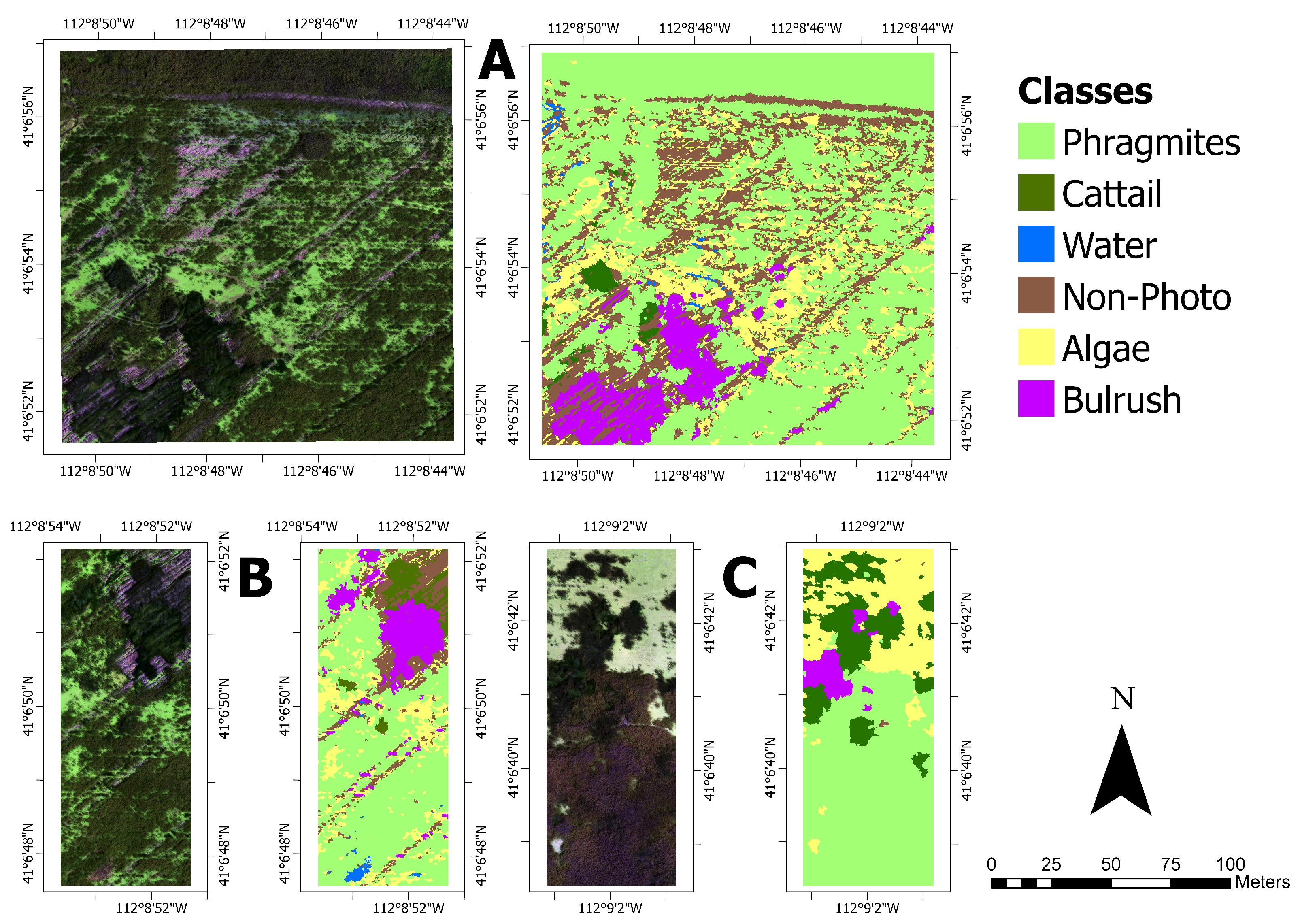
The training dataset (Figure 5A) was chosen to be representative of the entire orthomosaic. Phragmites dominated the study site, while native vegetation, cattail, and bulrush were minor constituents. Test site 1 (Figure 5B) contained a heterogeneous distribution of classes and similar class proportions to the training data. Due to less intensive management, the distribution of classes at test site 2 was more homogeneous than at test site 1, and test site 2 lacks the linear features found at the training site and test site 1 (Figure 5C). Notably, there was much more cattail, less non-photosynthetic material, and no water at test site 2 (Table 3).

2.4. CNN Semantic Segmentation

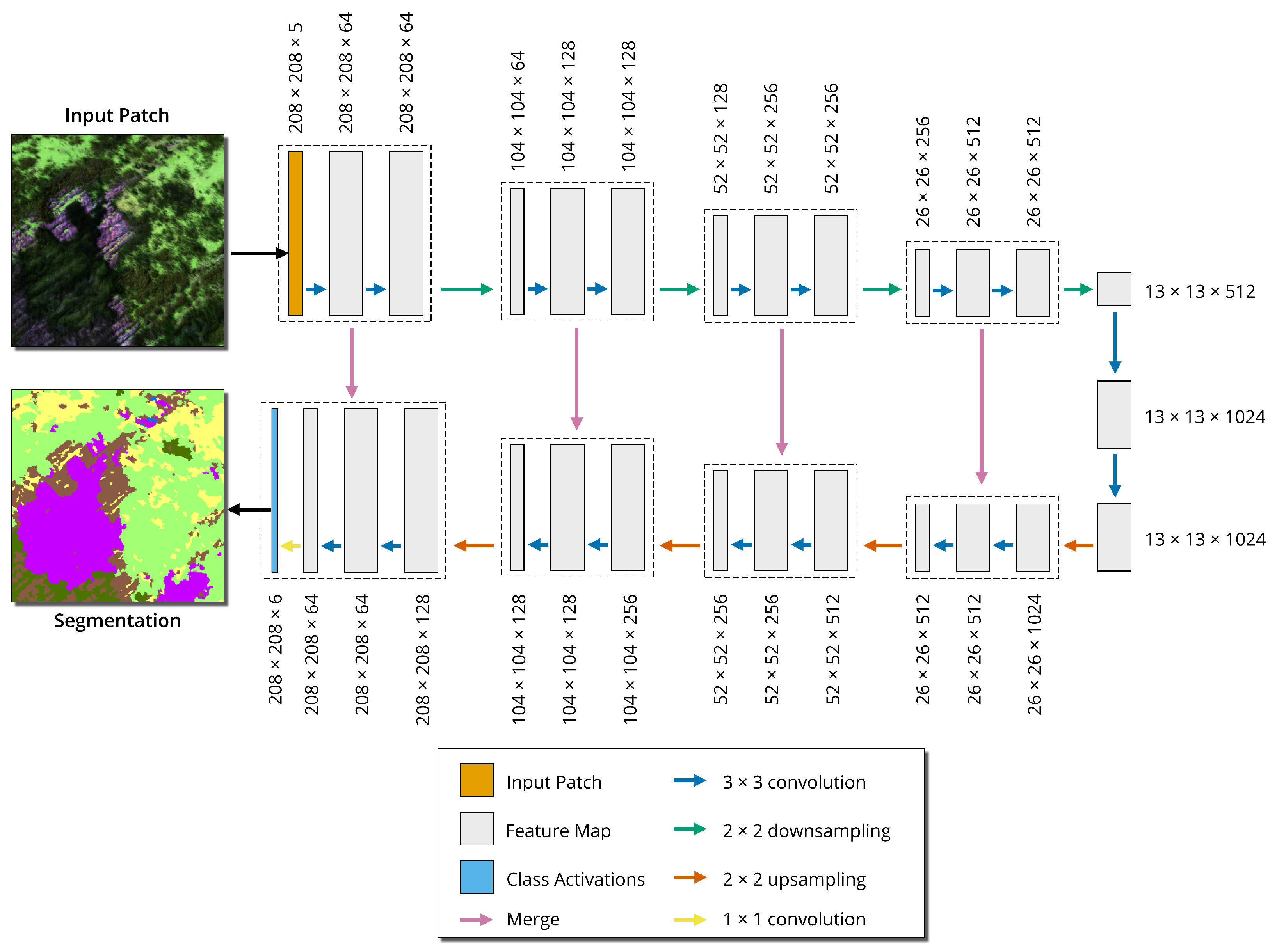
The CNN model was produced with ENVI version 5.6 and Deep Learning module version 1.1.2 (L3Harris Geospatial Solutions Inc., Boulder, CO, USA). ENVI Deep Learning implements a U-Net CNN architecture [26] with a TensorFlow backend, referred to as ENVINet5. The U-Net architecture is a popular type of CNN in remote-sensing-based semantic image classification [27]. The architecture is an encoder-decoder network, where the input images are downsampled several times by pooling layers, then upsampled with up-convolution layers to recover the spatial resolution. ENVINet5 has a total of 27 convolution layers and 5 ‘levels’, where each level is a different pixel resolution (Figure 6). ENVINet5 is patch-based; the full image is divided into smaller image patches, then dense prediction (all pixels within the patch are assigned a label) is performed on each patch. U-Net has several advantages over a traditional CNN. The architecture requires relatively few training samples to predict outcomes precisely. An overlap tile strategy is employed to allow for seamless prediction on large datasets. Data augmentation is possible to supplement limited training data and to make the model more generalizable. The model learns border pixels with a weighted loss [26]. Border pixels are where two objects’ borders meet, a complex region to define but essential for a spatially contiguous classification. The U-Net architecture was preferred because it is well-studied and has performance comparable to other state-of-the-art architectures [28].

U-Net CNN model parameters include patch size, augmentation scale, augmentation rotation, number of epochs, number of patches per batch, number of patches per epoch, patch sampling rate, class weight, and loss weight. The number of epochs (E) is given by Equation (1), where y is the scale factor.

$$E=300+5y^2$$

(1)

The number of epochs was increased as the image resolution decreased because there was less training data for the model to converge at a minimum loss value (

Table 4. The number of epochs for each resolution.

Resample Factor	Resolution (cm)	Train Image Width (Pixels)	Epochs
original	7.6	2171	305
2×	15.2	1086	320
3×	22.8	725	345
4×	30.4	543	380
5×	38.0	435	425
7×	53.2	311	545
10×	76.0	217	800

). Equation (1) was determined by experimentation to ensure each model converged. ENVI automatically sets the number of patches per batch and the number of patches per epoch because these parameters are impacted by the graphics card video random access memory (VRAM; Nvidia Tesla T4 with 16 GB of VRAM). The rest of the parameters were set to their default values and not varied; the augmentation scale and rotation were set to on, the patch size was 208 pixels, the number of patches per batch and number of patches per epoch were determined by ENVI, the patch sampling rate was 16, the class weight was 2, and the loss weight was 0.

Training a CNN model with the same data and parameters produces different classification results since their optimization is non-convex. There may be multiple global minima and a bad global minimum will cause poor generalization performance, which is reflected by poor accuracy on the test dataset [30]. This was increasingly the case as the spatial resolution coarsened and the amount of training data decreased. To account for variability in classification accuracy, three models were repeated for each scenario. There were 11 unique scenarios and three repetitions for each scenario for a total of 33 models.

2.5. Model Evaluation

The output models were evaluated using the two test datasets. An error matrix was produced for each test dataset, along with several accuracy metrics. As class-independent measures, the overall accuracy (Equation (2), where TP is true positive, TN is true negative, FP is false positive, and FN is false negative), kappa (Equation (3), where c is the class, N is the total number of classified pixels compared to reference pixels, m_c,c is the number of values belonging to reference pixels that have also been classified as class c, D_c is the total number of predicted values belonging to class c, and G_c is the total number of reference values belonging to class c; [31]), and mean F1 score (Equation (4), where p is precision and r is recall; [32]) metrics were used. For per-class measures, the precision (also known as user accuracy; Equation (5)) and recall (also known as producer accuracy; Equation (6)) were used.

$$OA=\frac{TP+TN}{TP+TN+FP+FN}$$

(2)

$$k=\frac{{\sum }_{c=1}^n{m}_{c,c}-{\sum }_{c=1}^n\left(G_c{D}_c\right)}{N^2-{\sum }_{c=1}^n\left(G_c{D}_c\right)}$$

(3)

$$F_{\mathrm{m}}=\frac{2}{\left|c\right|}\sum _c\frac{p_c\ast r_c}{p_c+r_c}$$

(4)

$$p=\frac{TP}{TP+FP}$$

(5)

$$r=\frac{TP}{TP+FN}$$

(6)

Accuracy metrics for the different spatial averaging methods (BOR and AOR) were compared with the Wilcoxon signed-rank test. The Wilcoxon test is a nonparametric test similar to the parametric paired t-test that compares the differences between two independent samples of the same community [33,34]. The test assumes that the differences are distributed symmetrically around the median [35]. The Wilcoxon test’s null hypothesis is that the median difference between paired samples is zero, and the alternative hypothesis is that the median difference between paired samples is not zero [36]. The testing was conducted at the alpha level of 0.01, where a significance test indicates that the method results are different. The tests were completed for each class-independent accuracy metric (overall accuracy, kappa, and the mean F1 score) at both test sites.

Tukey’s honestly significant difference (HSD) test was used to test for significant differences between the original and spatially averaged spatial resolutions’ class-independent accuracy metrics. The data were grouped by resolution, and the AOR and BOR methods were analyzed separately. Tukey’s HSD assumes that the data are normally distributed, the observations are independent, and variance is homogeneous in each group. The Shapiro–Wilkes test and Levene’s test were used to test for the normality and homogeneity of variance, respectively. These tests indicate that the data did not violate the assumptions of Tukey’s HSD at the alpha level of 0.01. A significance test (alpha = 0.01) of Tukey’s HSD indicates a difference between the original and spatially averaged resolutions. The tests were completed for each class-independent accuracy metric, overall accuracy, kappa, and the mean F1 score at both test sites.

3. Results

3.1. Image Stitching Results and Method Comparison

Figure 7 demonstrates the effects of each image resampling method. There was reduced contrast and spatial information for the BOR method at every resolution and a pixel shift from the original resolution orthomosaic. Pixels shifted south 21 cm for 2× resolution, east 53 cm for 3× resolution, southeast 18 cm for 4× resolution, and southeast 34 cm for 5× resolution at the location in Figure 7. The pixel shift varied in magnitude and direction, typically between 10 and 50 cm throughout each orthomosaic. The AOR method retained more spatial information and contrast and had no pixel shift from the original resolution. In Figure 7D,E, the loss of spatial information is apparent. The plant at the center of the road in Figure 7E (AOR method) is evident, while in Figure 7D (BOR method), it is less visible due to the loss of detail provided by the BOR method.

In Figure 8, the appearance of Phragmites and bulrush at 7.6, 22.8, 38.0, and 76.0 cm is compared. The differing texture of Phragmites is still apparent in the 22.8 cm spatially averaged imagery and barely visible in the 38.0 cm spatially averaged imagery. Meanwhile, bulrush has a wavy appearance because it tends to blow over in the wind at the flat wetland site. However, this texture is largely lost at a 22.8 cm resolution. Much of the structural information is lost for both classes by 76.0 cm; at this resolution, the models would have to largely rely on spectral information.

3.2. Model Performance at the Original Resolution

At test site 1 (Figure 5B), the average (±95% confidence interval) overall accuracy, kappa, and mean F1 score over three repetitions were 0.78 ± 0.01, 0.66 ± 0.02, and 0.63 ± 0.03, respectively. The model performed best for the Phragmites class with an F1 score of 0.89 ± 0.00 and worst for the cattail class with an F1 score of 0.16 ± 0.12. At test site 2 (Figure 5C), the average overall accuracy, kappa, and mean F1 score over three repetitions were 0.85 ± 0.01, 0.75 ± 0.03, and 0.63 ± 0.03, respectively. The model performed best for the algae class, with an F1 score of 0.95 ± 0.00, and worst for the non-photosynthetic class, with an F1 score of 0.10 ± 0.01. Notably, the mean overall accuracy among the three repetitions at test site 2 was 9.2% higher than at test site 1, while the mean F1 score decreased by 0.2%. The mean F1 score weighs each class the same, no matter the class prevalence. Test site 2 contained a small proportion of non-photosynthetic material (0.17%) that was poorly classified, resulting in dramatically different overall accuracy and mean F1 score values. The kappa values were between the overall accuracy and mean F1 score values at both test sites.

3.3. Comparison of Spatial Averaging Methods

The Wilcoxon signed-rank test was run between both resampling methods at 15.2 to 38.0 cm resolution and all three repetitions. At test site 1, the p-values were 0.73, 0.04, and 0.97 for the overall accuracy, kappa, and mean F1 score, respectively, so there was a failure to reject the null hypothesis (alpha = 0.01) that there was no significant difference between the BOR and AOR methods. At test site 2, the p-values were 0.18, 0.20, and <0.01 for the overall accuracy, kappa, and mean F1 score, respectively, so the null hypothesis was rejected for the mean F1 score but not rejected for the overall accuracy and kappa. This indicated that the mean F1 score may differ between the BOR and AOR methods at test site 2.

The BOR method performed notably worse for the bulrush class at test site 2 (58% difference in class F1 score), contributing to a lower mean F1 score (16% difference) when averaging the mean F1 score for all resolutions and repetitions. Meanwhile, the mean F1 scores were nearly identical (0.38% difference) when averaging the mean F1 score for all resolutions and repetitions at test site 1. These results could indicate that the spatial averaging method has a greater impact when the test site has a different distribution of classes from the training data. An example of model predictions at test site 1 is shown in Figure 9. At test site 2, cattail is much more prevalent than at the training site (17% compared to 1.1%). Additionally, cattails were more spectrally similar to bulrush, especially compared to Phragmites.

3.4. Model Performance at Different Spatial Resolutions

At test site 1, the AOR method had a consistent trend; the accuracy metrics decreased as the spatial resolution was increased. For the BOR method, the overall accuracy decreased for each step, while the kappa and mean F1 score values vary. At 30.4 and 38.0 cm, the BOR method outperformed the AOR method for kappa and mean F1 score, but the AOR method performed better with overall accuracy. The trend indicates that the BOR method performed better for less prevalent classes, while the AOR method performed better for more prevalent classes at this site. The per-class F1 score at test site 1 for each spatial resolution and spatial averaging method is shown in Figure 10.

The average class-independent accuracy metrics, percent difference from the original resolution, and Tukey’s HSD at test site 1 are displayed in

Table 5. The class-independent accuracy metrics with percent difference from the original resolution (7.6 cm) shown in parentheses at test site 1. Statistically significant results based on the p-value of Tukey’s HSD (alpha = 0.01) shown in bold.

	Test Site 1
	AOR Method			BOR Method
Resolution (cm)	Overall Accuracy	Kappa	Mean F1 Score	Overall Accuracy	Kappa	Mean F1 Score
7.6	0.78	0.66	0.63	0.78	0.66	0.63
15.2	0.75 (−4%)	0.62 (−6%)	0.58 (−8%)	0.74 (−5%)	0.59 (−11%)	0.57 (−10%)
22.8	0.74 (−5%)	0.61 (−8%)	0.56 (−11%)	0.69 (−11%)	0.51 (−23%)	0.52 (−18%)
30.4	0.70 (−11%)	0.56 (−15%)	0.54 (−15%)	0.71 (−8%)	0.56 (−15%)	0.57 (−9%)
38.0	0.64 (−18%)	0.50 (−24%)	0.53 (−15%)	0.66 (−15%)	0.49 (−25%)	0.55 (−13%)
53.2	0.62 (−20%)	0.46 (−31%)	0.44 (−30%)
76.0	0.58 (−26%)	0.41 (−39%)	0.45 (−28%)

. Each set of three repetitions at the degraded spatial resolutions was compared to three repetitions at the original spatial resolution. The AOR method had fewer significant results, and no accuracy metrics had significant results at 15.2 and 22.8 cm resolution. The BOR method had at least one significant result at each resolution. Between each method, the mean F1 score had the least number of significant results, indicating that class prevalence was not a major factor in reduced accuracy at the spatially averaged resolutions at test site 1.

At test site 2, the AOR method displayed an interesting result; between 22.8 and 30.4 cm spatial resolution, there was a large decrease in accuracy for each metric. The BOR method did not follow this trend. Instead, it followed a consistent pattern of reduced accuracy as the spatial resolution coarsened. The AOR method had relatively consistent accuracy metrics after the drop in accuracy. The drop in accuracy was attributed to a decrease in performance for all three vegetation species (Phragmites, cattail, and bulrush), while the BOR method was more consistent in performance for the vegetation species. The per-class F1 score at test site 2 for each spatial resolution and spatial averaging method is shown in Figure 11.

Table 6. The class-independent accuracy metrics with percent difference from original resolution (7.6 cm) shown in parentheses at test site 2. Statistically significant results based on the p-value of Tukey’s HSD (alpha = 0.01) shown in bold.

	Test Site 2
	AOR Method			BOR Method
Resolution (cm)	Overall Accuracy	Kappa	Mean F1 Score	Overall Accuracy	Kappa	Mean F1 Score
7.6	0.85	0.75	0.63	0.85	0.75	0.63
15.2	0.84 (−2%)	0.73 (−2%)	0.61 (−4%)	0.79 (−7%)	0.63 (−16%)	0.47 (−25%)
22.8	0.80 (−6%)	0.69 (−8%)	0.61 (−2%)	0.79 (−8%)	0.62 (−17%)	0.48 (−24%)
30.4	0.54 (−37%)	0.39 (−48%)	0.47 (−25%)	0.76 (−11%)	0.57 (−24%)	0.44 (−30%)
38.0	0.55 (−35%)	0.39 (−48%)	0.43 (−32%)	0.73 (−14%)	0.55 (−26%)	0.44 (−31%)
53.2	0.66 (−23%)	0.51 (−32%)	0.41 (−35%)
76.0	0.48 (−44%)	0.34 (−54%)	0.34 (−47%)

shows the average class-independent accuracy metrics, percent difference from the original resolution, and Tukey’s HSD at test site 2. Test site 2 had more significant results compared to test site 1. Notably, the BOR method had significant results at all spatially averaged resolutions. The AOR method was not significant until 30.4 cm resolution. At this site, there was a greater magnitude of difference between the overall accuracy and the mean F1 score for the BOR method, while the metrics were similar for the AOR method.

For the AOR method, kappa usually had the greatest decrease from the original resolution result. This is likely because the decrease in accuracy is trending closer to the ‘random chance’ model that the kappa metric considers. For the BOR method, the overall accuracy and mean F1 score showed different trends depending on the test site. At test site 1, the overall accuracy rapidly decreased while the mean F1 score varied and was more similar to the original resolution result. At test site 2, the overall accuracy slowly decreased, while the mean F1 score had a large difference at all resolutions. The BOR method had a poor recall value for the cattail and bulrush classes, indicating many false negatives. Simultaneously, the precision for Phragmites was lower than the recall, indicating a higher proportion of false positives for Phragmites. At test site 2, the BOR method overpredicted for Phragmites and underpredicted for native vegetation such as cattail and bulrush.

4. Discussion

The U-Net CNN model had relatively good performance at the original resolution even though this study did not prioritize best performance. To isolate the effect of spatial resolution, this study omitted common practices to improve classification accuracy for individual models, such as model pretraining and hyperparameter tuning, instead opting for a uniform training approach. While U-Net is an established CNN-based model in the literature, there are other model architectures that may offer improved performance. Cheng et al. [37] developed ISNet, a deep learning network for improved separability of the boundaries between semantics. Zhang et al. [38] created a transformer and CNN hybrid deep neural network for the semantic segmentation of very-high-resolution imagery. This work sought to establish a baseline comparison of CNN-based model performance using a well-studied architecture, U-Net; however, future work should study model performance of new approaches, such as those of Cheng et al. [37] and Zhang et al. [38], at different spatial resolutions.

The BOR spatial averaging method was a more accurate representation of independently acquired imagery at a coarser spatial resolution. While only the mean F1 score at test site 2 was significantly different than the AOR Method, the BOR method generally had worse performance compared to the original resolution with more statistically significant differences and, frequently, lower accuracy. There were three main contributors to the reduced model accuracy: the reduction in spatial information, the geolocation accuracy between the resampled imagery and reference data, and the lower quality of image stitching during orthomosaic production. It is unknown how much each factor contributes to reduced model performance. For this reason, the BOR processed imagery could be considered a worst-case scenario and the AOR processed imagery a best-case, while it is most likely that model performance with newly collected imagery at a coarser resolution would fall somewhere between the two.

In addition to the loss of spatial detail at coarser resolutions, the amount of training data also decreased. At a 76.0 cm resolution, the 217 × 217 pixel training image provided about 1% as much training data as the original resolution (7.6 cm) 2171 × 2171 pixel training image. It is rather impressive that the CNN model could converge on a prediction for the 76.0 cm resolution imagery, achieving nearly 60% overall accuracy at both test sites. It is evident that a 76.0 cm resolution was too coarse for the categorical scale used in this study (species-level classification). Additionally, it would have been difficult to visually interpret imagery coarser than the original (7.6 cm) to create training data, even if there were more ground-collected reference data.

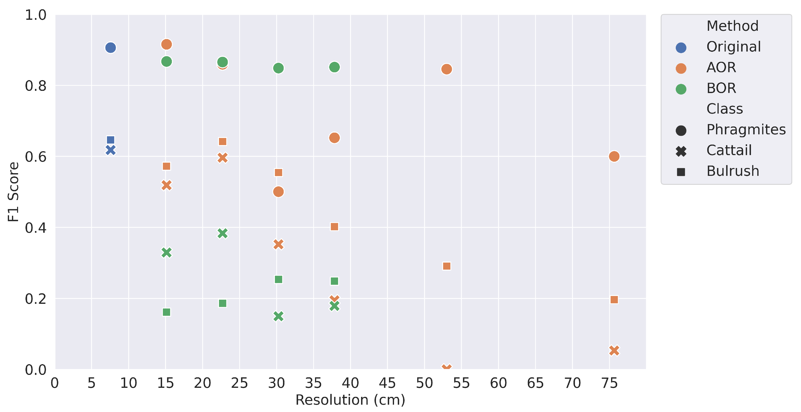
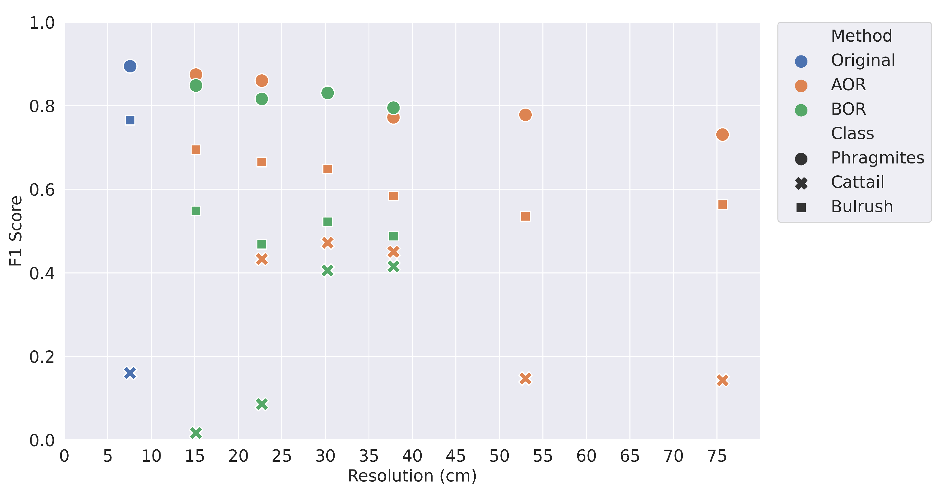
The classification accuracy on a per-class basis demonstrates the importance of plant morphology. The overall accuracy was almost always highest for Phragmites, and the precision and recall values showed no trends of over or under prediction. The Phragmites at the site were seeding, creating a texture distinct from bulrush and cattail. Bulrush was also distinct, with thinner leaves and a tendency to blow over in the wind. Cattail shared characteristics of both Phragmites and bulrush from the aerial imagery, as some of the cattails were seeding, causing confusion with Phragmites, but the spectral response was more similar to bulrush, also causing confusion with bulrush. Additionally, cattail was a minor constituent of the field site, only covering 1.1% of the training site. As a result, the classification accuracy was lowest for cattail, which had consistently low recall values. The low classification accuracies for cattail underscores the importance of class prevalence. In most cases, cattail had the lowest F1 score, regardless of spatial resolution. There is a potential that an analysis with a spatial resolution finer than 7.6 cm could provide further insights. Several studies, such as Fromm et al., Neupane et al., and Schiefer et al. [13,14,15], have applied CNNs at finer resolutions as small as 0.3 cm. For instance, perhaps more detail is required to accurately map cattail, and class prevalence is not the sole issue. There would also be more training samples available. With a 0.76 cm resolution, there would be 100× more pixels than at 7.6 cm resolution. Again, the reduction in ground sample distance will reduce the flight coverage area, so such a reduction would be more appropriate for highly targeted scenarios or potentially a multi-scale analysis.

Based on our results, coarsening the spatial resolution from 7.6 cm to 22.8 cm in this study area could allow for increased spatial coverage or reduce image acquisition time while only moderately reducing accuracy. Acquisition time represents a significant cost and limits mapping large study areas at fine spatial resolutions. Processing software provides an additional cost tradeoff that should be considered before undertaking similar projects. This research relied on commercial software (Pix4D and ENVI) requiring licensing that may be prohibitively expensive for small projects. Free and open source alternatives exist, such as OpenDroneMap [39] for image stitching and Tensorflow [40] or PyTorch [41] for modeling, but require additional experience and/or programming skills.

The evaluation of this study was based on geographically stratified test sites. In an ideal situation, a stratified random sample would be generated to meet the basic statistical assumption. In this case, random points would be generated across the entire study site, then an image patch would be produced, centered at this point. However, the ground reference data were limited (Figure 4), and it would have been difficult to visually interpret the ground reference labels throughout the entirety of the image, causing additional human error. Considering the coarser resolution imagery and a patch size of 208 pixels, a stratified random sample would require a much larger study area and time investment for field data collection and image labeling.

The CNN architecture used in this study did not convolve the spectral dimension of the image data. With only five bands, a three-dimensional CNN would be unlikely to appreciably improve accuracy over the results shown here. However, the impacts of the spectral resolution and the number of bands on classification accuracy should be further explored in future research. While this work demonstrates a decrease in accuracy as spatial resolution coarsens, additional spectral information may improve differentiation between vegetation species [42,43]. Hyperspectral image data could maintain high accuracy even at coarser spatial resolutions, effectively sidestepping tradeoffs between spatial resolution, areal coverage, and classification accuracy; however, hyperspectral sensors are typically more costly than RGB or multispectral sensors. Recent work has demonstrated applying three-dimensional CNNs to hyperspectral imagery for tree species classification [44,45]. Hyperspectral UAS data can provide a complementary assessment of species cover when combined with coarser resolution hyperspectral data, as demonstrated for wetland vegetation by Bolch et al. [42].

5. Conclusions

This study has demonstrated a negative correlation between spatial resolution and CNN-based model accuracy; as spatial resolution becomes coarser, classification accuracy decreases. However, there is potential for similar model performance between the original 7.6 cm resolution imagery and spatial resolutions up through 22.8 cm resolution imagery based on simulated imagery. The slight decrease in model accuracy between these resolutions may be worth the potential tradeoff for greater coverage area. At resolutions coarser than 22.8 cm, there is less confidence that a deep learning model can reliably predict at the plant species level in this ecosystem.

While each land cover classification project is unique, and there is no optimal spatial or spectral resolution for every situation, the lessons learned here can be broadly applied. The land cover types at a study site may require a certain level of spatial and spectral detail for a CNN-based model to learn patterns. In this study, seeding Phragmites required less detail than bulrush, and, consequently, the classification accuracy of Phragmites was higher than bulrush at coarser spatial resolutions. The level of detail required by the land covers will influence the UAS flight parameters. At coarser resolutions, there was low confidence in the cattail and bulrush classes and much confusion between the two. Finally, it is essential in project planning to find the best balance between spatial detail and the amount of coverage area. The capture rate originally used in this project—1.2 km²/day—could cause difficulties outside of highly targeted projects. In this case study of species-level classification of graminoid plants, a 22.8 cm resolution and 10.8 km²/day capture rate could offer better balance between classification accuracy and spatial coverage.

References

1. Vaz, A.S.; Alcaraz-Segura, D.; Campos, J.C.; Vicente, J.R.; Honrado, J.P. Managing plant invasions through the lens of remote sensing: A review of progress and the way forward. Sci. Total Environ. 2018, 642, 1328–1339. [Google Scholar] [CrossRef] [PubMed]
2. Markham, B.L.; Townshend, J.R.G. Land cover classification accuracy as a function of sensor spatial resolution. In Proceedings of the Fifteenth International Symposium on Remote Sensing of Environment, Ann Arbor, MI, USA, 11–15 May 1981; pp. 1075–1090. [Google Scholar]
3. Ju, J.; Gopal, S.; Kolaczyk, E.D. On the choice of spatial and categorical scale in remote sensing land cover classification. Remote Sens. Environ. 2005, 96, 62–77. [Google Scholar] [CrossRef]
4. Ma, L.; Liu, Y.; Zhang, X.; Ye, Y.; Yin, G.; Johnson, B.A. Deep learning in remote sensing applications: A meta-analysis and review. ISPRS J. Photogramm. Remote Sens. 2019, 152, 166–177. [Google Scholar] [CrossRef]
5. Cheng, G.; Yang, C.; Yao, X.; Guo, L.; Han, J. When Deep Learning Meets Metric Learning: Remote Sensing Image Scene Classification via Learning Discriminative CNNs. IEEE Trans. Geosci. Remote Sens. 2018, 56, 2811–2821. [Google Scholar] [CrossRef]
6. Liu, T.; Abd-Elrahman, A.; Zare, A.; Dewitt, B.A.; Flory, L.; Smith, S.E. A fully learnable context-driven object-based model for mapping land cover using multi-view data from unmanned aircraft systems. Remote Sens. Environ. 2018, 216, 328–344. [Google Scholar] [CrossRef]
7. Kattenborn, T.; Lopatin, J.; Förster, M.; Braun, A.C.; Fassnacht, F.E. UAV data as alternative to field sampling to map woody invasive species based on combined Sentinel-1 and Sentinel-2 data. Remote Sens. Environ. 2019, 227, 61–73. [Google Scholar] [CrossRef]
8. Qian, W.; Huang, Y.; Liu, Q.; Fan, W.; Sun, Z.; Dong, H.; Wan, F.; Qiao, X. UAV and a deep convolutional neural network for monitoring invasive alien plants in the wild. Comput. Electron. Agric. 2020, 174, 9. [Google Scholar] [CrossRef]
9. Zhang, C.; Atkinson, P.M.; George, C.; Wen, Z.; Diazgranados, M.; Gerard, F. Identifying and mapping individual plants in a highly diverse high-elevation ecosystem using UAV imagery and deep learning. ISPRS J. Photogramm. Remote Sens. 2020, 169, 280–291. [Google Scholar] [CrossRef]
10. Higgisson, W.; Cobb, A.; Tschierschke, A.; Dyer, F. Estimating the cover of Phragmites australis using unmanned aerial vehicles and neural networks in a semi-arid wetland. River Res. Appl. 2021, 37, 1312–1322. [Google Scholar] [CrossRef]
11. Onishi, M.; Ise, T. Explainable identification and mapping of trees using UAV RGB image and deep learning. Sci. Rep. 2021, 11, 903. [Google Scholar] [CrossRef]
12. Kattenborn, T.; Leitloff, J.; Schiefer, F.; Hinz, S. Review on Convolutional Neural Networks (CNN) in vegetation remote sensing. ISPRS J. Photogramm. Remote Sens. 2021, 173, 24–49. [Google Scholar] [CrossRef]
13. Fromm, M.; Schubert, M.; Castilla, G.; Linke, J.; McDermid, G. Automated Detection of Conifer Seedlings in Drone Imagery Using Convolutional Neural Networks. Remote Sens. 2019, 11, 2585. [Google Scholar] [CrossRef] [Green Version]
14. Neupane, B.; Horanont, T.; Hung, N.D. Deep learning based banana plant detection and counting using high-resolution red-green-blue (RGB) images collected from unmanned aerial vehicle (UAV). PLoS ONE 2019, 14, e0223906. [Google Scholar] [CrossRef]
15. Schiefer, F.; Kattenborn, T.; Frick, A.; Frey, J.; Schall, P.; Koch, B.; Schmidtlein, S. Mapping forest tree species in high resolution UAV-based RGB-imagery by means of convolutional neural networks. ISPRS J. Photogramm. Remote Sens. 2020, 170, 205–215. [Google Scholar] [CrossRef]
16. Cracknell, A.P. Review article Synergy in remote sensing-what’s in a pixel? Int. J. Remote Sens. 1998, 19, 2025–2047. [Google Scholar] [CrossRef]
17. Huang, C.; Townshend, J.R.G.; Liang, S.; Kalluri, S.N.V.; DeFries, R.S. Impact of sensor’s point spread function on land cover characterization: Assessment and deconvolution. Remote Sens. Environ. 2002, 80, 203–212. [Google Scholar] [CrossRef]
18. Wang, Q.; Atkinson, P.M. The effect of the point spread function on sub-pixel mapping. Remote Sens. Environ. 2017, 193, 127–137. [Google Scholar] [CrossRef] [Green Version]
19. Dorji, P.; Fearns, P. Impact of the spatial resolution of satellite remote sensing sensors in the quantification of total suspended sediment concentration: A case study in turbid waters of Northern Western Australia. PLoS ONE 2017, 12, e0175042. [Google Scholar] [CrossRef]
20. Roth, K.L.; Roberts, D.A.; Dennison, P.E.; Peterson, S.H.; Alonzo, M. The impact of spatial resolution on the classification of plant species and functional types within imaging spectrometer data. Remote Sens. Environ. 2015, 171, 45–57. [Google Scholar] [CrossRef]
21. Schaaf, A.N.; Dennison, P.E.; Fryer, G.K.; Roth, K.L.; Roberts, D.A. Mapping Plant Functional Types at Multiple Spatial Resolutions Using Imaging Spectrometer Data. GIScience Remote Sens. 2011, 48, 324–344. [Google Scholar] [CrossRef]
22. Matheson, D.S.; Dennison, P.E. Evaluating the effects of spatial resolution on hyperspectral fire detection and temperature retrieval. Remote Sens. Environ. 2012, 124, 780–792. [Google Scholar] [CrossRef]
23. Beauchemin, S.S.; Bajcsy, R. Modeling and Removing Radial and Tangential Distortions in Spherical Lenses. In Multi-Image Analysis; Springer: Berlin/Heidelberg, Germany, 1999; pp. 1–21. [Google Scholar]
24. Esri. Segmentation. Available online: https://pro.arcgis.com/en/pro-app/latest/help/analysis/image-analyst/segmentation.htm (accessed on 18 April 2022).
25. Comaniciu, D.; Meer, P. Mean shift analysis and applications. In Proceedings of the Seventh IEEE International Conference on Computer Vision, Kerkyra, Greece, 20–27 September 1999; pp. 1197–1203. [Google Scholar]
26. Ronneberger, O.; Fischer, P.; Brox, T. U-Net: Convolutional Networks for Biomedical Image Segmentation. In Medical Image Computing and Computer-Assisted Intervention—MICCAI 2015; Springer International Publishing: Cham, Switzerland, 2015; Volume 9351, pp. 234–241. [Google Scholar]
27. Pan, Z.; Xu, J.; Guo, Y.; Hu, Y.; Wang, G. Deep Learning Segmentation and Classification for Urban Village Using a Worldview Satellite Image Based on U-Net. Remote Sens. 2020, 12, 1574. [Google Scholar] [CrossRef]
28. Torres, D.L.; Feitosa, R.Q.; Happ, P.N.; La Rosa, L.E.C.; Junior, J.M.; Martins, J.; Liesenberg, V. Applying Fully Convolutional Architectures for Semantic Segmentation of a Single Tree Species in Urban Environment on High Resolution UAV Optical Imagery. Sensors 2020, 20, 563. [Google Scholar] [CrossRef] [Green Version]
29. L3 Harris Geospatial. Pixel Segmentation Training Background. Available online: https://www.l3harrisgeospatial.com/docs/PixelSegmentationTrainingBackground.html (accessed on 22 May 2022).
30. Neyshabur, B.; Bhojanapalli, S.; McAllester, D.; Srebro, N. Exploring generalization in deep learning. In Proceedings of the 30th International Conference on Neural Information Processing Systems, Long Beach, CA, USA, 4–9 December 2017. [Google Scholar] [CrossRef]
31. L3 Harris Geospatial. ENVI Confusion Matrix Kappa Coefficient. Available online: https://www.l3harrisgeospatial.com/docs/enviconfusionmatrix__kappacoefficient.html (accessed on 18 April 2022).
32. Hammerla, N.Y.; Halloran, S.; Ploetz, T. Deep, Convolutional, and Recurrent Models for Human Activity Recognition using Wearables. In Proceedings of the Twenty-Fifth International Joint Conference on Artificial Intelligence (IJCAI-16), New York, NY, USA, 9–16 July 2016. [Google Scholar] [CrossRef]
33. Nhu, V.H.; Mohammadi, A.; Shahabi, H.; Ahmad, B.B.; Al-Ansari, N.; Shirzadi, A.; Clague, J.J.; Jaafari, A.; Chen, W.; Nguyen, H. Landslide Susceptibility Mapping Using Machine Learning Algorithms and Remote Sensing Data in a Tropical Environment. Int. J. Environ. Res. Public Health 2020, 17, 4933. [Google Scholar] [CrossRef] [PubMed]
34. Scheff, S. Fundamental Statistical Principles for the Neurobiologist; Academic Press: Cambridge, MA, USA, 2016. [Google Scholar] [CrossRef]
35. Taheri, S.M.; Hesamian, G. A generalization of the Wilcoxon signed-rank test and its applications. Stat. Pap. 2013, 54, 457–470. [Google Scholar] [CrossRef]
36. LaMorte, W.W. Wilcoxon Signed Rank Test; Boston University School of Public Health: Boston, MA, USA, 2017. [Google Scholar]
37. Cheng, G.; Wang, G.; Han, J. ISNet: Towards Improving Separability for Remote Sensing Image Change Detection. IEEE Trans. Geosci. Remote Sens. 2022, 60, 5623811. [Google Scholar] [CrossRef]
38. Zhang, C.; Jiang, W.; Zhang, Y.; Wang, W.; Zhao, Q.; Wang, C. Transformer and CNN Hybrid Deep Neural Network for Semantic Segmentation of Very-High-Resolution Remote Sensing Imagery. IEEE Trans. Geosci. Remote Sens. 2022, 60, 4408820. [Google Scholar] [CrossRef]
39. OpenDroneMap. ODM—A Command Line Toolkit to Generate Maps, Point Clouds, 3D Models and DEMs from Drone, Balloon or Kite Images. Available online: https://github.com/OpenDroneMap/ODM (accessed on 22 May 2022).
40. Abadi, M.; Agarwal, A.; Barham, P.; Brevdo, E.; Chen, Z.; Citro, C.; Corrado, G.S.; Davis, A.; Dean, J.; Devin, M.; et al. TensorFlow: Large-Scale Machine Learning on Heterogeneous Systems. 2015. Available online: tensorflow.org (accessed on 22 May 2022).
41. Paszke, A.; Gross, S.; Massa, F.; Lerer, A.; Bradbury, J.; Chanan, G.; Killeen, T.; Lin, Z.; Gimelshein, N.; Antiga, L.; et al. PyTorch: An Imperative Style, High-Performance Deep Learning Library. In Advances in Neural Information Processing Systems 32; Wallach, H., Larochelle, H., Beygelzimer, A., d’Alché-Buc, F., Fox, E., Garnett, R., Eds.; Curran Associates, Inc.: Red Hook, NY, USA, 2019; pp. 8024–8035. [Google Scholar]
42. Bolch, E.A.; Hestir, E.L.; Khanna, S. Performance and Feasibility of Drone-Mounted Imaging Spectroscopy for Invasive Aquatic Vegetation Detection. Remote Sens. 2021, 13, 582. [Google Scholar] [CrossRef]
43. Cawse-Nicholson, K.; Townsend, P.A.; Schimel, D.; Assiri, A.M.; Blake, P.L.; Buongiorno, M.F.; SBG Algorithms Working Group. NASA’s surface biology and geology designated observable: A perspective on surface imaging algorithms. Remote Sens. Environ. 2021, 257, 11234. [Google Scholar] [CrossRef]
44. Mäyrä, J.; Keski-Saari, S.; Kivinen, S.; Tanhuanpää, T.; Hurskainen, P.; Kullberg, P.; Poikolainen, L.; Viinikka, A.; Tuominen, S.; Kumpula, T.; et al. Tree species classification from airborne hyperspectral and LiDAR data using 3D convolutional neural networks. Remote Sens. Environ. 2021, 256, 2. [Google Scholar] [CrossRef]
45. Zhang, B.; Zhao, L.; Zhang, X. Three-dimensional convolutional neural network model for tree species classification using airborne hyperspectral images. Remote Sens. Environ. 2020, 247, 11193. [Google Scholar] [CrossRef]
Figure 1. Satellite imagery of the flight area (red crosshatch) in the Howard Slough Waterfowl Management Area.
Remotesensing 14 02703 g001
Figure 2. Field-collected images of the classes at the study site.
Remotesensing 14 02703 g002
Figure 3. Examples of each land cover class from the orthomosaic. Each tile has been contrast stretched to highlight differences in texture: (A) Phragmites; (B) cattail; (C) bulrush; (D) non-photosynthetic; (E) water; (F) algae.
Remotesensing 14 02703 g003
Figure 4. A map of ground reference points and reference sites within the study area. The background image is the 7.6 cm true color composite of UAS imagery acquired in August 2020.
Remotesensing 14 02703 g004
Figure 5. Training and testing image and label sets for model training and evaluation: (A) Training site; (B) Test site 1; (C) Test site 2.
Remotesensing 14 02703 g005
Figure 6. ENVINet5 model architecture, adapted with permission from Ref. [29]. Copyright 2022, L3Harris Geospatial Solutions, Inc. The orange box represents the input patch, the gray box represents a feature map, the blue box represents the class activations with one per class (6 total), the pink arrow indicates a merge (also known as a skip connection), the blue arrow indicates a 3 × 3 convolution, the green arrow indicates 2 × 2 downsampling, the orange arrow indicates 2 × 2 upsampling, and the yellow arrow indicates a 1 × 1 convolution.
Remotesensing 14 02703 g006
Figure 7. True color image examples of spatial averaging methods: (A) Original resolution (7.6 cm); (B) 2× (15.2 cm) resolution created using before orthomosaic resampling (BOR); (C) 2× resolution created using after orthomosaic resampling (AOR); (D) 5× (38.0 cm) resolution BOR; (E) 5× resolution AOR.
Remotesensing 14 02703 g007
Figure 8. A comparison of Phragmites and bulrush appearance at different resolutions with coarsened imagery simulated using the AOR method: (A) The original resolution, 7.6 cm; (B) 3× resolution (22.8 cm); (C) 5× resolution (38.0 cm); (D) 10× resolution (76.0 cm). The texture of Phragmites (left of red line) provided a distinct appearance, even at a coarser resolution, while the ‘wavy’ texture of bulrush (right of red line) was apparently lost.
Remotesensing 14 02703 g008
Figure 9. Classification images at test site 1: (A) the reference data (7.6 cm); (B) model prediction at the original resolution (7.6 cm); (C) model prediction at 5× resolution (38.0 cm) using the AOR method; (D) model prediction at 5× resolution (38.0 cm) using the BOR method.
Remotesensing 14 02703 g009
Figure 10. The F1 score for each vegetation class by spatial averaging method at test site 1. The vegetation classes are represented by shapes; circle is Phragmites, cross mark is cattail, and square is bulrush. The spatial averaging methods are represented by colors; blue is original, orange is after orthomosaic resampling (AOR), and green is before orthomosaic resampling (BOR). The BOR method performs worse than the AOR method with cattail and bulrush.
Remotesensing 14 02703 g010
Figure 11. The F1 score for each vegetation class by spatial averaging method at test site 2. The vegetation classes are represented by shapes; circle is Phragmites, cross mark is cattail, and square is bulrush. The spatial averaging methods are represented by colors; blue is original, orange is after orthomosaic resampling (AOR), and green is before orthomosaic resampling (BOR). The BOR method again performs worse than the AOR method for the cattail and bulrush classes but has a higher F1 score than the AOR method for Phragmites at 30.4 and 38.0 cm resolution.
Remotesensing 14 02703 g011