Abstract
Landslide displacement prediction is an essential base of landslide hazard prevention, which often needs to establish an accurate prediction model. To achieve accuracy prediction of landslide displacement, a displacement prediction model based on a salp-swarm-algorithm-optimized temporal convolutional network (SSA-TCN) is proposed. The TCN model, consisting of a causal dilation convolution layer residual block, can flexibly increase the receptive fields and capture the global information in a deeper layer. SSA can solve the hyperparameter problem well for TCN model. The Muyubao landslide displacement collected from a professional GPS monitoring system implemented in 2006 is used to analyze the displacement features of the slope and evaluate the performance of the SSA-TCN model. The cumulative displacement time series is decomposed into trend displacement (linear part) and periodic displacement (nonlinear part) by the variational modal decomposition (VMD) method. Then, a polynomial function is used to predict the trend displacement, and the SSA-TCN model is used to predict the periodic displacement of the landslide based on considering the response relationship between periodic displacement, rainfall, and reservoir water. This research also compares the proposed approach results with the other popular machine learning and deep learning models. The results demonstrate that the proposed hybrid model is superior to and more effective and accurate than the others at predicting the landslide displacement.
1. Introduction
Landslides are common natural geological disasters that cause a lot of property loss and personal injury every year [1,2]. The landslide early warning system (LEWS), including real-time monitoring methods such as remote sensing (RS), the global position system (GPS), and the geographic information system (GIS), is an effective approach to identify the early displacement and development trend of landslides [3,4,5]. The landslide surface displacement prediction based on real-time monitoring data is an important part for LEWS [6,7]. It can provide advanced landslide displacement information to decision makers, which reduces the damage caused by landslides. Therefore, the accurate prediction of landslide displacement can be an effective method to reduce landslide risks.
Numerous approaches have been developed for the purpose of landslide displacement prediction. They can be divided into two main types: physically-based approaches and data-driven approaches [8,9,10]. Among these models, the physically-based models mainly take geotechnical characteristics into analysis and quantify the slope displacement by combining the slope stability calculation and seepage theory [11,12]. The physically-based models predict landslide displacement by using physical properties that provide a good understanding of the slope displacement. However, these models require detailed geomorphological data, but the physical parameters are often uncertain and difficult to properly define for a large-scale landslide. On the contrary, a large number of the availability data with high-precision provided by the landslide monitoring system promote the development and application of data-driven models. With the rapid development of artificial intelligence approaches, machine learning and deep learning models have been attracting increasing attention for landslide displacement prediction. Hence, these intelligence models, such as artificial neural networks (ANN) [13], support vector machines (SVM) [14], extreme learning machines (ELM) [15], and long short-term memory (LSTM) [16] have constructed a relationship between induced triggers and landslide displacement. However, the characteristics of landslide displacement time series are affected by the complexity of its own geological conditions and the randomness and suddenness of external factors. So, the “step-like” displacement usually contains the linear and nonlinear displacement components. The intelligence models may not able to simultaneously predict linear and nonlinear components well [17,18]. An idea in previous study is to combine a nonlinear intelligent model with the total displacement decomposition method for surface displacement prediction [19,20,21]. The total displacement of the landslide is decomposed into different linear and nonlinear subsequences according to different triggering factors of the landslide. For example, Lian et al. [19] introduced ensemble empirical mode decomposition (EEMD) to decompose the original displacement time series into several sub-series, Ren et al. [22] extracted the trend and periodic displacements from the initial displacement by the discrete wavelet transform (DWT), and Guo et al. [13] decomposed the accumulation displacement into trend and periodic displacements by variational mode decomposition (VMD) according to the physical meaning. In this study, we applied the time-series decomposition method to reduce the complexity of the original displacement, and then suitable models were used to predict the different displacement subsequences; the final result was obtained by reconstructing each predicted subsequence value.
The above models provide effective methods for landslide displacement prediction. Especially, the sequence deep learning model RNNs, including two import variants of long short-term memory (LSTM) and gated recurrent unit (GRU), have superior performance to the others for landslide displacement prediction [16,23,24]. Although the RNNs can capture temporal associations from time series data for displacement prediction, the sequence construction and memory gates slow down the sequence processing and use up a lot of memory to store calculation results. Moreover, as a sequence model, the RNNs fail at global modeling [25]. Among the deep learning models, CNN is another popular research object and has performed well in many fields [26,27]. CNNs have good ability to learn local features from neighboring points in Euclidean space and have gained attention for time-series forecasting recently [28]. However, their application in landslide displacement requires more research. The temporal convolutional network (TCN) [29] is a variant architecture of CNN combined with the time-series modeling ability of RNN and CNN’s global feature extraction. TCN used for time-series processing can focus on some important features in the history sequence from a global perspective and extract these features through its own autonomous learning. Hence, the TCN convolutional time-series prediction model was introduced to mine the temporal relationship in the long-term monitoring data. Moreover, a deep learning model usually contains a complexity structure neural network. It is not easily trained compared with the traditional machine model. The swarm intelligence algorithm is a distributed bionic algorithm with random search characteristics inspired by the social behavior of natural groups [30,31]. So, in the model building process, an intelligent algorithm called the salp swarm algorithm (SSA) [32], which does not need to adjust a specific optimizer, was applied for the optimization the parameters of the TCN model.
The main contributions of the present study are summarized as follows: (i) a hybrid model based on TCN model was proposed for displacement prediction. (ii) The linear and the nonlinear parts of the total displacement were extracted by a time-series decomposition method that can reduce the complexity of the time series. (iii) A large-scale landslide with step-like displacement behavior in the TGRA of China was used to validate the feasibility and effectiveness of the proposed model.
2. Methodologies
2.1. Convolutional Neural Network (CNN)
Convolutional neural networks are widely applied in extracting features from multiple dimensions data with Euclidean space [33,34]. A typical CNN model consists of a convolution layer, an activation layer, a pooling layer, and a fully connected layer. On the convolution layer, a set of trainable filters slide over the input data to perform a convolution operation and extract features; they are called feature maps. The individual units in feature maps correspond to the local positions of original input that the filter currently covers [35] (Figure 1). In addition, at every local region of input data, the convolution filter uses the same weights. This is the weight-sharing strategy, which can reduce the complexity of the convolution layer and the number of parameters that are required to be trained. The pooling layers usually follow the convolution layer, and adjacent information in the feature maps is merged by max pooling, average pooling, or other operations. Finally, the fully connected layer is used to transform the features processed by convolution and pooling layers into one-dimensional vectors for conveniently processing and outputting results. The activation layer puts nonlinear functions into the neural network, which can improve the nonlinear expression ability of the model. The commonly used activation equations are the Sigmiod function, the ReLu function, and the Tanh function, etc. Actually, according to different tasks and dimensions of input, data that needs to be processed by CNN can be divided into three different dimensions network structures. The one-dimensional CNN (1D-CNN) model is used for sequential data and is applicable to signal processing problems. The time-series data were processed as different channels data that not only can build nonlinear relationships between different input features but also merge nearby time-step data by the convolution layer and pooling layer in the 1D-CNN model. So, the 1D-CNN model can extract temporal features from original sequence data. The two-dimensional CNN (2D-CNN) model is mainly used for image and text recognition, and the three-dimensional CNN (3D-CNN) model is used for video data. Thus, in this study, the 1D-CNN model was also applied in landslide displacement prediction for competition with the TCN model.
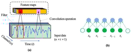
Figure 1.
(a) The 1D-CNN model structure. (b) The convolution operation with kernel size k = 3.
2.2. Temporal Convolutional Network (TCN)
The TCN module is a new and unique CNN model that combines the advantages of the time-series modeling capabilities of RNN and CNN’s parallel processing. In particular, the core components of TCN contain two causal dilated convolution layers and a residual block. The causal convolution layer stresses the order for sequence processing, and the dilated convolution layer can flexibly adjust the size of the receptive filed in TCN. The residual block is an effective method that can avoid the degradation of the deep network [36].
2.2.1. Causal Dilation Convolution Layer
Causal convolutions are convolutions where the output at time t can only depend on the inputs that are no later than time t, as shown in Figure 2a. However, the insufficient receptive of the causal convolution layer has a limited ability to capture global information. In order to capture much longer sequence information, the dilation strategy through interval sampling is applied to obtain larger perception. For a given input 1-D dimension sequence x, the output at time t of the dilation convolution layer can be defined as:
where the s is the output and f is a 1-D dimension filter with size k. ∗ is the convolution operation, d is the dilation factor, and t − d · i indicates the cells covered in the perspective field. The dilation factor d and the filter size k in the TCN can flexibly adjust the size of the receptive filed to obtain features of the input sequence with different time scales. Figure 2b shows an example of the dilation strategy, where the filter size is two and the interval sampling period d = 1, 2.
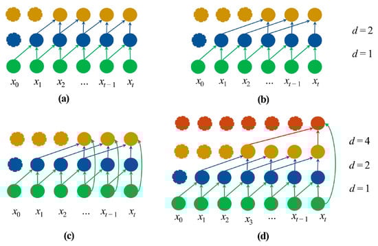
Figure 2.
The architectural components in a TCN module. (a) Causal convolution with kernel size k = 2. (b) Dilated convolution with dilation factors d = 1, 2. (c) Residual block. (d) A schematic of the TCN module with dilated causal convolution and a residual block.
2.2.2. Residual Block
The residual block can be expressed as that the original input of the TCN module is added to the output of the causal dilation convolution layer, and then the addition is output by an activation function (Figure 2c). The residual block can be calculated as
where x and o are the input and output of the TCN module; F represents a series of operations, including causal dilated convolution, and activation function. In order to make the input x with the same size of F(x), the 1 × 1 convolution layer is added to express the input. So, the Equation (2) can summarized as follows:
2.3. Total Displacement Decomposition Based on Variational Mode
Previous works [20] indicated that the cumulative displacement of the landslide was affected by the internal geological conditions (lithology, structural conditions, topography, etc.) and external environment factors (rainfall, reservoir water level). The step-like displacement of landslide is a non-stationary time-series varying with time, which can be divided into trend displacement and periodic displacement. Geological conditions are the main factor affecting the trend displacement, and the curve of trend displacement shows an approximate monotonous increasing trend for a long period. The displacement fluctuation in a short period is affected by external environmental factors. Therefore, the accumulated displacement can be decomposed as follows:
where t is the time, xt is the accumulated displacement, st is the trend displacement, and pt is the periodic displacement.
Variational mode decomposition (VMD) is a signal decomposition technology using a non-recursive decomposition mode [37]. Based on convergence conditions, it can control the number of modes obtained by original data. Assuming that each mode has a limited bandwidth and is compacted around their respective center frequencies, the goal is to minimize the sum of the bandwidth of each mode. The constraint is that the sum of the mode functions vk is equal to the original signal. The mathematical description of the variational problem is as follows:
where is the vector of the center frequency on the complex plane, vk represents the mode function, ωk is the center frequency of each component, and f is the original data.
In order to solve the constrained variational problem, a quadratic penalty term and lagrange multiplier are used to transform the problem unconstrained. The augmented lagrangian, L, is depicted as follows:
where α is the penalty factor and λ is the lagrange multiplier.
In the process of solving the constrained variational problems, the alternating direction multipliers method (ADMM) is used to constantly update vk, ωk, and λ for finding the saddle point of the lagrange expression, that is, the solution of the above equation. The adaptive decomposition of the signal is completed according to the frequency domain characteristics of the original signal [38].
2.4. Salp Swarm Algorithm
Salp swarm algorithm (SSA) [32] is a global optimization algorithm based on swarm biological intelligence proposed in recent years. The SSA simulates the movement and foraging behavior of salp chain in nature [39]. The salps are divided into two subgroups equally, named leaders and followers, respectively. Assuming that there is a food source F in the N-dimensional search space, the leaders are the salp individuals with the most abundant information on F. The positions of the leaders are located at the begin of the salp chain usually. The positions of followers are updated based on the leaders or other followers. In the process of looking for food, the information about the food source F obtained is also constantly updated. For the leaders, the movement method is carried out according to the following formula:
where shows the position of the i-th salp (leader) in the j-th dimension, ; m is the number of salps; Fj is the position of the food source in the j-th dimension; and ubj and lbj are the upper and lower bounds in the same dimension, respectively. c2 and c3 are generated randomly in range (0, 1), and c1 is calculated as follows:
where t is the current iteration step and tmax is the max number of iteration step. c1 is decreased during the iteration process for strengthening the different capabilities of the algorithm in different search stages.
The position of the followers is updated according to the following equation:
where shows the position of i-th follower in j-th dimension, .
2.5. Hybrid TCN Forecasting Model and Implementation Procedure
In this study, we present a hybrid model that uses the swarm intelligence algorithm as a parameter optimizer to automatically determine the hyperparameters for the TCN model. Compared with the machine learning model, the complicated model of deep learning requires extensive trial and error when determining the structure of the model. The SSA has an efficient search strategy and strong spatial search ability, which are likely to provide greater possibilities to obtain global optimal solutions. Any application of the swarm intelligence algorithm should meet two basic requirements: (i) a defined function, which can converse input to output; (ii) an evaluation indexed for an individual solution [40]. The optimizing deep learning model with the SSA meets the above requirements in the following two respects:
(1) The deep learning model is often regarded as a ‘black box’ model. Although it is difficult to give specific mathematical expressions, the model is still a one-to-one correspondence between input and output when the weights and biases are determined. In this study, each individual in the SSA will be a potential solution for setting the hyperparameters of the TCN model. An individual in SSA can be expressed as a real vector S. For example, in TCN, the hyperparameters such as the kernel size, the number of kernels, and the number of neural units should be contained in S.
(2) The evaluation scheme is used to calculate the fitness value of each potential solution to determine the performance of the solution. In this study, the root mean squared error (RMSE) is chosen to evaluate the solution. Moreover, the mean absolute percentage error (MAPE) and correlation coefficient (R) are also adopted to verify the performance of the predictive model. These error criteria methods are defined as:
where si and represent the measured and predicted values; and represent the mean of observed and predicted values; and n is the number of predicted values.
The implementation procedure of the hybrid model based on TCN for “step-like” displacement prediction is summarized as follows.
Step 1: Randomly generate solutions in the k-dimensional search space.
Step 2: Introduce the solution S as hyperparameters of TCN model and train the TCN model on the training dataset.
Step 3: Evaluate the prediction results by calculating the fitness value of term RMSE on the validation dataset and sort all the solutions based on the fitness value. The solution corresponding to the optimal fitness value is assigned to F.
Step 4: Update the position of the leading and follower salps separately by the update formulas in Section 2.4.
Step 5: Repeat steps (2)–(4) until a termination criterion is met.
Step 6: Return the TCN predictive model.
Based on the time-series decomposition method mentioned above, we proposed a temporal convolutional network (TCN) optimized by SSA as shown in Figure 3. Firstly, the total displacement of the landslide is decomposed into two displacement sub-sequences named periodic term and trend term. The trend term is fitted and predicted by a polynomial function. Through the analysis of the monitoring data, the external candidate factors that trigger the periodic displacement are preliminarily selected, and the maximal information coefficient (MIC) [41] method is used to quantitatively determine the correlation value between the candidate factors and periodic displacement. The SSA is applied to optimize the hyperparameters of the TCN model. Then, the trained model is used to predict the periodic component displacement. The predicted result of the cumulative displacement is the sum of the predicted periodic displacement and trend displacement.
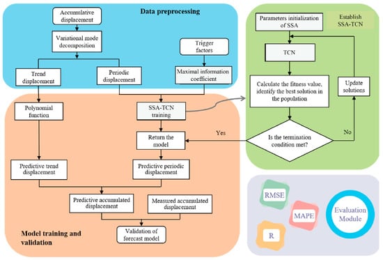
Figure 3.
The flowchart of the proposed forecast model.
3. Case Study
3.1. Topography and Geology of the Muyubao Landslide
The Muyubao landslide on the slope of the south bank of the Yangtze River is located in the county of Zigui country of Hubei province, 56 km away from the Three Gorges Dam (Figure 4a). The average annual rainfall in this study region is 1493.2 mm. The rainfall is concentrated from July to September, counting 70% of the cumulative rainfall each year. The Muyubao landslide is a large-scale unstable slop that includes a volume of 96 million m3 sliding mass, an area of 1.8 km2. The landslide has a maximum north-to-south length of about 1500 m and an average width of about 1200 m on the different direction (Figure 4b). The upper boundary of the landslide is at an elevation of 540 m above sea level (a.s.l.), and the toe of the landslide dips into the Yangtze River at 100 m (a.s.l.). The upper portion of the landslide shows a steep slope gradient of nearly 25° and gently lowers with the elevation decrease. The sliding mass is mainly composed of a surficial quaternary deposit and fractured quartz sandstone, as shown in Figure 4c. The surficial deposit is composed of silty clay and rubble, which makes up 40–60% of the total volume. The thickness of sliding mass ranges from 60 m to 120 m, and the front part is an uplift platform formed by shear sliding with a thickness of 80~120 m. The main sliding direction of the landslide is 20°, which faces the Yangtze River. The bedrock mainly consists of Jurassic siltstone and Triassic quartz sandstone with dip directions of 27° and dip angles of 25°. The sliding zone is a thickness of 0.1 to 0.3 m layer of dark-gray to black coal and shale that extends along the interface between the bedrock and the sliding mass [42,43].
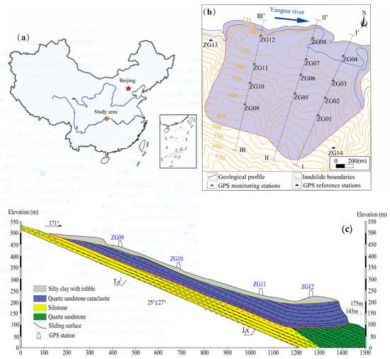
Figure 4.
(a) The location of the study area in China; (b) the monitoring network of the Muyubao landslide; (c) the geological profile III-III’ of the Muyubao landslide.
3.2. Displacement Characteristics Analysis
The landslide displays slow creep character before the initial TGR impoundment (June 2003), and activity signs including the ground fracture and infrastructure damage occurred rarely. However, by the filling-drawdown cycle of the reservoir level after 2003, the landslide deformation is gradually obvious, especially after the first trial impoundment to 156 m a.s.l. (November 2006). Since then, a total of 12 GPS points is set up on the Muyubao landslide in a regular form of three rows and four columns for surface displacement monitoring. The distribution of monitoring points is depicted in Figure 4b, and the other two reference stations (ZG12 and ZG13) are located on stable rock, which is out of the sliding area. The GPS is a kind of GNSS that can provide millimeter accuracy for landslide displacement monitoring [44]. The long-term GPS displacement monitoring results in Figure 5 indicated that most of the area of Muyubao exists at a similar displacement rate (except for ZG01, which is affected by the topography conditions). The displacement around section Ⅰ-Ⅰ’ is the most significant, with a total displacement of 2447.9 mm (ZG01), 1693.0 mm (ZG02), 1678.9 mm (ZG03), and 1756 mm (ZG04). The displacement recorded by ZG05, ZG06, ZG07, and ZG08 around the central section of Ⅱ-Ⅱ’ of the landslide are similar at cumulative displacement between 1560 mm with 1630 mm and an average velocity of about 10.96 mm/month. Compared with the other points, the displacement data measured by the four GPS station sites around profile III-III’ on the west of the landslide show the lowest displacement, with an average cumulative displacement of 1521 mm. During the whole 12-year monitoring period, the horizontal displacement of the Muyubao landslide displays a linear creep character, but several significant displacement events were observed in the overall monitoring period. There are four evident acceleration events (2007, 2008, 2012, and 2017); each rapidly increased event was usually during a periodic of approximately 5 months (from November to April of the following year). During the four periods, the displacement increased approximately 30% of the total displacement observed in the December 2018. Moreover, the landslide displacement rapidly increased corresponding to the periods of relatively higher reservoir water level every year, while during the rest of the year, the landslide displacement experienced a slower increase, which corresponds to the relatively lower reservoir level period.
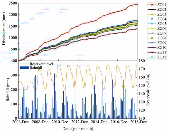
Figure 5.
The monitoring data of cumulative displacement, the reservoir water level, and rainfall in the Muyubao landslide.
4. Model Implementation
4.1. Displacement Decomposition Result
Through a detailed observation of the displacement time series, several displacement curves can be found with similar displacement trend such as ZG02 and ZG03, ZG05 and ZG06, ZG07 and ZG08, ZG10 and ZG11, and ZG04 and ZG12. Hence, the other two points (ZG01, ZG09) and the five typical points (ZG03, ZG06, ZG08, ZG11, and ZG12) from each pair of GPS points with similar displacement were selected to evaluate the performance of the proposed method. These typical points were located around the three geological profiles (I-I’, II-II’ and III-III’) from the trailing edge to the former edge which can respect to the displacement status of the whole slope. For each GPS point, a total of 146 displacement samples were obtained by monthly recording from November 2006 to December 2018. In order to clearly provide the results of the proposed method in this study, in the following parts, the calculation results visualized in figures were based on the three points (ZG01, ZG06, and ZG12), and all seven points of the calculation results were specifically presented in tables. Figure 6 shows the trend and periodic displacement time-series that were extracted by VMD. The curves with approximately linear growth correspond to the trend displacements. The curves with high fluctuation frequency correspond to the periodic displacement components and show a similar one-year cycle of displacement characterized by acceleration from October to March or April of the following year and descending during April to September. During the four acceleration events (2007, 2008, 2012, and 2017), the average increments of periodic displacements were 50.72 mm, 72.32 mm, 81.27 mm, and 71.27 mm, and the average monthly trend displacements were 24.63 mm, 19.96 mm, 14.87 mm, and 15.13 mm, respectively. In the rest of these years, the average monthly trend displacements were 15.58 mm, 19.08 mm, 16.49 mm, and 12.53 mm, respectively. The trend displacement increase rates were similar even during the period with a displacement rapid increase, so the trend displacements can show an approximate line increase.
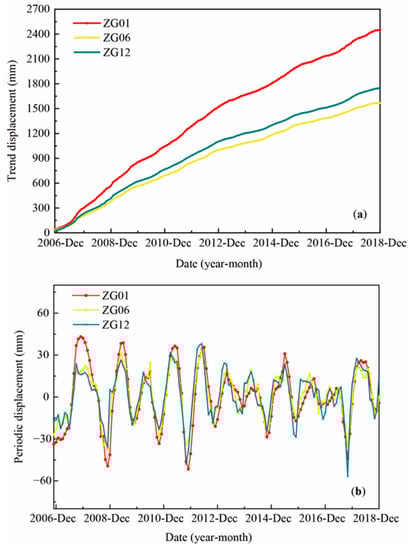
Figure 6.
The extracted displacements from ZG01, ZG06, and ZG12 by VMD. (a) Trend displacements; (b) periodic displacements.
4.2. Data Preparation
The monitoring data collected from November 2006 to December 2017 of the selected seven points are chosen as the training sample, and the test samples contain the data from January to December 2018 test samples. The standardization function is used to standardize the training sample and test sample, respectively. The standardization function is calculated as
where x′ is the standardization result, x is the original value, and u and σ are the sample mean and sample standard deviation of the selected dataset.
4.3. Analysis the Influencing Factors of Periodic Displacement
As the input of the periodic displacement prediction model, the trigger factor plays a key role in influencing the output of the final result. Hence, it is necessary to analyze the relationship between the influence factors and the periodic displacement. According to the aforementioned analysis, the landslide displacement shows a certain correlation with the rainfall and reservoir water level. The effect of reservoir operations on slope stability can be divided into a seepage effect or buoyancy effect [42]. The former can be regarded as the dynamic water seepage effect caused by the imbalance of the water levels in the changing process of the reservoir water level. The latter can be considered as the buoyancy effect by submerging different volumes of the slope to reduce effective stress. So, the average reservoir level in the previous month (a1) and the change of reservoir level during the last 1 month (a2) are considered as influencing factors on the reservoir water. The rainfall effect contributes to the destabilization of the soil by replenishing the groundwater and reducing effective stresses. The rainfall effect can be divided into “lateral flow” and “vertical flow” [45]. The lateral flow is considered as affecting the stability of the slope in the mid to long term timescale, and the vertical flow works in the short term [46]. Therefore, the candidate factors affecting rainfall on different timescales include the monthly rainfall (b1) and the cumulative rainfall of the last 2 months (b2). On the other hand, the different evolution states of the landslide make the displacement of the landslide respond differently to the external triggering factors [47,48]. The evolution status of the landslide can be obtained through the history movement information of the landslide. Moreover, the valuable information may be mined from the extracted displacements and velocities to predict the periodic displacement. Therefore, the velocity of cumulative displacement (c1) and the velocity of the periodic displacement (c2) are also selected as candidate factors.
The displacement of slope is usually considered as a complex multi-dimension nonlinear system at spatiotemporal scale [49]. The complexity and uncertainty of the geological conditions and the randomness and suddenness of external factors are the two main aspects that impart the nonlinear characteristics to the displacement system. Correlation coefficients, such as Pearson’s correlation coefficient, are usually used as feature selection algorithms due to their simple but practical character. However, these methods cannot usually provide a nonlinear relationship between inducing factors and displacement [50]. The maximal information coefficient (MIC) based on the statistical method is used for capturing the correlation between two variables. MIC not only calculates linear and non-linear correlations but also can identify important and difficult-to-recognize correlations [41,51]. Hence, the MIC was applied to identify and screen the environmental factors that induce landslide displacement in this research. The MIC value is between 0 and 1. If two variables show strong dependence, the MIC value is close to 1. Otherwise, it will tend to 0. Figure 7 presents linear and nonlinear relationships (MIC values) among the selected factors and the displacement at selected points of the Muyubao landslide. The MIC values of all candidate factors are equal to or greater than 0.2, revealing the strong correlation relationship between candidate factors and periodic displacement. So, the six candidate factors are selected as the input factors to predict the periodic displacements. In the following, the six factors data were constructed into a six-channel data, and each channel was used to input one factor time-series data, which is similar to the input data shown in Figure 1a, which can be processed by the TCN and 1D-CNN models.
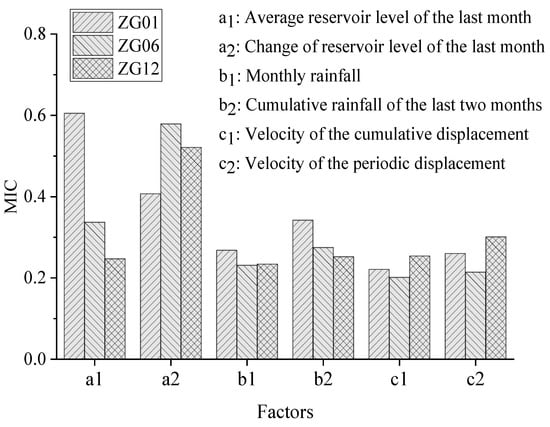
Figure 7.
The MIC values between the periodic displacement and candidate factors.
4.4. Hyper-Parameters and Models Training
In this research, a series experiments were coded by python 3.6 and implemented on a personal computer (CPU: AMD Ryzen 5 2400G 3.6 GHz, 8 GB), including the proposed model and the other comparison models in the later section. In the TCN module, the receptive fields were directly affected by the dilation factors d and the kernel size (k). Insufficient reception hinders the extraction of long-term history information, while the excessively large receptive files increase the calculation burden. Hence, the SSA optimizer were used to determine the hyper-parameters and the model training parameters of the TCN model. In this study, there are six initial input channels of TCN, which corresponds to the number of input factors. Moreover, three causal dilation layers were constructed for the TCN module, and the dilation factors were set to {1, 2, 4}. The kernel size (K), the number of filters (Nf), and the initial learning rate (lr) were optimized by SSA. The specific search space of the hyperparameters was defined as a space R7 ∈ [1, 6]3 × [1, 64]3 × [0.0001, 0.05]. For the SSA optimizer, the population size and iteration epochs are 20 and 200, respectively. The loss function was RMSE, and the iteration process was stopped when the loss of validation dataset was minimized. In comparison, the other two models that has performed well in the landslide displacement prediction (i.e., SVM, LSTM) [22,52] and the 1D-CNN model were applied in competition with the proposed model. The SSA was used to determine the hyperparameters of the three comparison models, and the specific parameters are shown in the Table 1. For the LSTM model, parameter Nu represents the LSTM unit number, and Nl represents the number of layers of the LSTM. In the SVM model, the kernel function was set to “rbf”, with the parameters C and γ representing the regularization parameter and the kernel parameter, respectively. In the 1D-CNN model, the hyperparameters Nk, Kc represent the number of kernels and the kernel size in the convolution layer, respectively.

Table 1.
The hyperparameters of TCN and the three comparison models.
5. Results and Discussion
5.1. Prediction Results
5.1.1. Trend Displacement Prediction
The trend displacement is a smooth monotone increasing sequence (Figure 6a). A polynomial with five orders is used to fit the trend displacement in the training sample. The least squares method is applied to find the best fitting values for the parameters of the polynomial function. The polynomial function is as follows:
where yt is the fitted values of the trend term displacement at the time t, and a, b, c, d, e, and f are the coefficients, where a cannot be zero.
The fitting polynomial of degree five and the prediction results of the trend displacements are shown in Figure 8 and Table 2. As exhibited in Figure 8, all the polynomials of degree five can accurately fit the increasing trend of landslide displacements and predict the following development in the test datasets. The R values of ZG01, ZG03, ZG06, ZG08, ZG09, ZG11, and ZG12 on the test samples are 0.991, 0.991, 0.982, 0.989, 0.989, 0.984, and 0.990, respectively. The fitting results of the trend displacements are close to the monitored displacement, mainly because the VMD can reduce the complexity of the original data and obtain relatively stable displacement components.
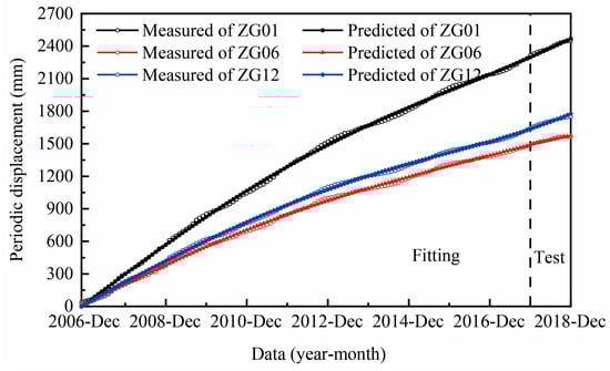
Figure 8.
A comparison of the predicted and measured trend displacements.
Table 2.
The coefficients of the trend displacement polynomial function (Equation (14)).
5.1.2. Periodic Displacement Prediction
According to the parameters setting the result in Section 4.4, the TCN prediction model was established. Figure 9 and Table 3 exhibit the prediction results produced by the trained models and compared with the measured values. It clearly shows that the prediction results of the TCN model have a similar fluctuation to the measured displacements. Most of the prediction values are close to the measured displacements. For the seven selected sites, the average values of RMSE, MAPE, and R on the test samples are 6.37 mm, 1.487%, and 0.911, respectively. The prediction results compared with the monitoring displacements indicate that the TCN model runs well on the periodic displacement prediction. In short, the TCN is a suitable tool for building nonlinear relationships between the external factors and the periodic displacement.
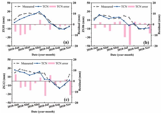
Figure 9.
A comparison of the predicted and measured displacements: (a) ZG01, (b) ZG06, and (c) ZG12.
Table 3.
The errors of the predicted results of the TCN model.
5.1.3. Cumulative Displacement Prediction
The period displacement prediction component and the trend term displacement prediction component are added to obtain the cumulative displacement prediction value of the landslide. From January to December 2018, the average values of RMSE, MAPE, and R of TCN are 15.89 mm, 0.85%, and 0.922, respectively (Table 4). Figure 10 shows that the predicted cumulative displacements based on the polynomial of degree five and the TCN model are in good agreement with the measured displacement of the monitoring points. This is due to the hybrid models providing an integrated learning strategy, which can reduce the complexity of the time-series displacement, and relatively simple nonlinear and nonlinear models can realize high accuracy prediction.
Table 4.
The cumulative displacement prediction accuracy.
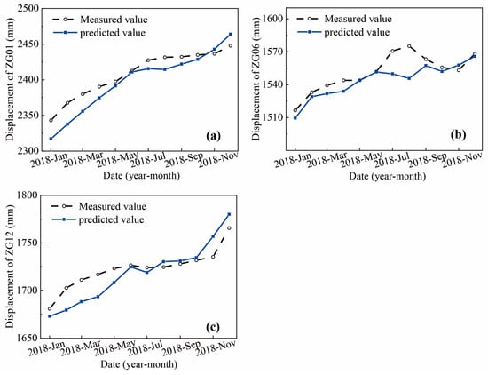
Figure 10.
The predicted and measured cumulative displacements at (a) ZG01, (b) ZG06, and (c) ZG12.
In the early monitoring period, the step-like displacement is obvious, but the step-like displacement feature is not significant at the end of the monitoring period. Compared with the different displacement status, we think the effect of the fluctuation of the reservoir water level on the slope will be weakened in the future. Other slopes with similar monitoring data in the Three Gorges Reservoir area also illustrate this point, such as the Baishuihe landslide [53] and the Qianjiangping landslide [54]. The surface displacement prediction is an import part of LEWS; the slope failure warning criterion is usually based on the displacement value and corresponding indices including the displacement rate, the displacement tangent angle and the inverse velocity method [55,56]. The displacement value cannot consistently produce an accurate slope failure warning for a certain landslide at present, due to the complexity and uncertainty of the geological conditions and external factors. However, these critical criteria of landslide failure can be obtained by accurate displacement prediction results, which can contribute to evacuating people from risk slop in advance and reduce landslide risk. So, in the future we will concentrate on the critical criterion of landslide failure, based on this method.
5.2. Periodic Displacement Prediction Comparison among Different Models
5.2.1. Comparing the 1D-CNN Model with the TCN Model
Although few studies introduce the CNN algorithm to perform landslide displacement prediction, it has useful applications in many other time-series prediction fields. So, in this competition, we constructed a 1D-CNN model for periodic displacement prediction, and three statistical metrics—RMSE, MAPE, and R—are used to evaluate the performance of the 1D-CNN and TCN models. Figure 11 and Table 5 show the specific comparison results. In Table 5, both the 1D-CNN and TCN models can provide relatively good accuracy of the periodic displacements, indicating that the 1D-CNN model also has potential to simulate landslide periodic displacement for LEWS. However, among 21 evaluation indices of the 7 points, 15 indices of the TCN model are superior to the 1D-CNN model. This indicates that the sequence processing abilities in the TCN model can improve the competitiveness for time-series prediction. Compared with the 1D-CNN model, the prediction accuracy of the TCN model improved by 18.22%, −21.93%, 13.73%, 11.60%, 14.64%, 10.89%, and 1.56%, respectively, for the RMSE index. For MAPE, the relative improvements are 88.55%, −32.00%, 43.02%, 22.51%, 36.17%, −5.71%, and −74.58%, respectively. For the R index, the relative improvements are 9.45%, −2.23%, −5.45%, 4.08%, 1.95%, 6.94%, and 0.46%, respectively. To sum up, compared with the results of the 1D-CNN model, the average relative improvement ratios of RMSE, MAPE, and R of TCN are 7.95%, 32.27%, and 2.10%, respectively. So, compared with 1D-CNN model, the TCN model was recommended for the periodic displacement prediction.
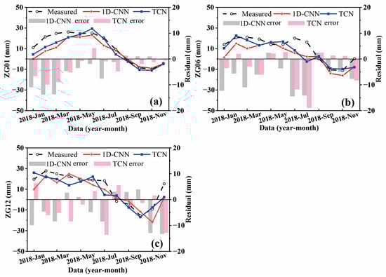
Figure 11.
A comparison of monitored and predicted periodic landslide displacements using the 1D-CNN and TCN prediction models for different points: (a) ZG01, (b) ZG06, and (c) ZG12.
Table 5.
The periodic displacements prediction accuracy among the 1D-CNN and TCN models for the seven points.
5.2.2. Comparison among TCN, LSTM, and SVM
To further evaluate the performance of the proposed model, the TCN model was compared with the SVM and LSTM models, which have performed well for displacement prediction too. The specific comparison results of the prediction performance indices are shown in Table 6, and the prediction values for the testing sample are shown in Figure 12. Generally, the three proposed models can predict the trend of the monitoring displacements. However, for the SVM model, the error and fluctuation compared with the monitoring displacement are larger than the other two models. From Table 6, compared with the static SVM model, the time-series modeling models (LSTM and TCN) are more competitive and reach a relatively high prediction accuracy. This result is consistent with the previous findings that the dynamic modeling method performed better than the static model [16,23,24]. Moreover, on most of the testing sites, the TCN model was outperformed by the other models. The performance of the LSTM model was lower than the TCN model in this competition. Specifically, compared with the SVM model, the average improvement ratios of RMSE, MAPE, and R of TCN were 39.58%, 66.69%, and 8.99%, respectively. For the LSTM model, the average improvement ratios of RMSE, MAPE, and R of TCN were 8.35%, 17.25%, and 0.56%, respectively.
Table 6.
The periodic displacement prediction accuracy among the SVM, LSTM, and TCN models for the selected seven points.
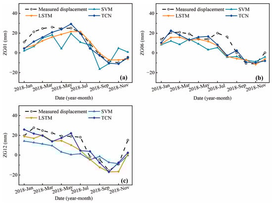
Figure 12.
A comparison of monitored and predicted periodic displacements using three prediction models for different sites: (a) ZG01, (b) ZG06, and (c) ZG12.
In this competition, we also computed the time consumption for training the SVM, LSTM, and TCN models. The suitable SVM parameters were searched for using a meta-heuristic SSA, and the parameters in the TCN and LSTM models were optimized based on the gradient descent algorithm (Adam). The training time for SVM (10.26 s) is lower than the LSTM (15.15 s) and TCN (11.57 s) models because there were only two parameters optimized by SSA, which was much less than the number of parameters in the two time-series models. Compared with the LSTM model, the training consumption of TCN decreased by 23.63%. The main reason for this is that the parameters in the filters of the TCN model are shared across a convolution layer and a pooling layer, which can reduce the number of parameters. In particular, the LSTM is a sequence model, a lot of gate units were used to memorize the history information, and the calculation of the later state needs to wait for the former state calculation to be completed [25,57]. These results support the effectiveness of the proposed TCN model in processing the time series and improving the prediction accuracy, especially for periodic displacement.
6. Conclusions
Based on the long-term professional GPS monitoring in the Muyubao landslide, a large-scale landslide in the TGRA of the chain, this study proposed a hybrid method of step-like landslide displacement prediction based on the TCN model, which consists of causal dilation layers and a residual block. The time-series analysis and the VMD theory were used to decompose the cumulative displacement, reduce the complexity of the data, and obtain relatively clear displacement patterns. For cumulative displacement prediction, the average values of RMSE, MAPE, and R of the proposed method are 15.89 mm, 0.85%, and 0.922, respectively. The results indicate that the prediction values of the proposed model are in good agreement with the actual values.
Moreover, this study focuses on the periodic displacement prediction, which is difficult to use to predict final prediction results. The periodic displacement prediction results indicated that the average RMSE (6.37 mm), MAPE (1.49%), and R (0.911) of the TCN model were the best, compared with the two commonly used machine learning and deep learning methods (SVM and LSTM). Compared with the static SVM model, the average improvement ratios range from 8.99% to 66.69%; compared with the sequence model LSTM, the accuracy of the proposed TCN model improved from 0.56% to 17.25%. Moreover, the training time of the TCN decreases by 23.63% compared with LSTM model. This is due to the TCN combined with the time-series modeling ability of RNN and CNN’s global feature extraction. Convolution and pooling layers are widely applied in the TCN model, which can extract global features and reduce the number of parameters by using a weight-sharing strategy. The causal dilation layer in TCN can flexibly increase the receptive fields in the deeper layer, which contributes to the longer memory time series. Overall, the feasibility and superiority of the proposed hybrid method are demonstrated by successful implication in the seven landslides displacement time-series prediction. The proposed method can decompose cumulative displacement into relatively simple displacement components that are also suitable for other landslide displacement predictions characterized by slow-moving deformation and step-like displacements effected by periodical or seasonal factors.
Author Contributions
Conceptualization, D.H. and Y.S.; methodology, D.H., J.H. and Y.S.; software, J.H. and Y.S.; validation, Z.G. and Y.S.; resources, D.H.; writing—original draft preparation, J.H.; and writing—review and editing, X.H. and Y.G. All authors have read and agreed to the published version of the manuscript.
Funding
The research was supported by the National Natural Science Foundation of China (Nos. 41972297 and 41902290), by a supporting program of a hundred promising innovative talents in the Hebei provincial education office (No. SLRC2019027), and by the Natural Science Foundation of Hebei Province (No. D2020202002 and D2021202002).
Data Availability Statement
Not applicable.
Conflicts of Interest
The authors declare no conflict of interest.
References
- Froude, M.J.; Petley, D.N. Global fatal landslide occurrence from 2004 to 2016. Nat. Hazard. Earth Syst. 2018, 18, 2161–2181. [Google Scholar] [CrossRef] [Green Version]
- Kirschbaum, D.B.; Adler, R.; Hong, Y.; Hill, S.; Lerner-Lam, A. A global landslide catalog for hazard applications: Method, results, and limitations. Nat. Hazards 2009, 52, 561–575. [Google Scholar] [CrossRef] [Green Version]
- Zhu, Z.-W.; Liu, D.-Y.; Yuan, Q.-Y.; Liu, B.; Liu, J.-C. A novel distributed optic fiber transduser for landslides monitoring. Opt. Lasers Eng. 2011, 49, 1019–1024. [Google Scholar] [CrossRef]
- Tofani, V.; Raspini, F.; Catani, F.; Casagli, N. Persistent Scatterer Interferometry (PSI) Technique for Landslide Characterization and Monitoring. Remote Sens. 2013, 5, 1045–1065. [Google Scholar] [CrossRef] [Green Version]
- Barra, A.; Solari, L.; Béjar-Pizarro, M.; Monserrat, O.; Bianchini, S.; Herrera, G.; Crosetto, M.; Sarro, R.; González-Alonso, E.; Mateos, R.; et al. A Methodology to Detect and Update Active Deformation Areas Based on Sentinel-1 SAR Images. Remote Sens. 2017, 9, 1002. [Google Scholar] [CrossRef] [Green Version]
- Petley, D.N.; Mantovani, F.; Bulmer, M.H.; Zannoni, A. The use of surface monitoring data for the interpretation of landslide movement patterns. Geomorphology 2005, 66, 133–147. [Google Scholar] [CrossRef]
- Yin, Y.; Wang, H.; Gao, Y.; Li, X. Real-time monitoring and early warning of landslides at relocated Wushan Town, the Three Gorges Reservoir, China. Landslides 2010, 7, 339–349. [Google Scholar] [CrossRef]
- Corominas, J.; Moya, J.; Ledesma, A.; Lloret, A.; Gili, J.A. Prediction of ground displacements and velocities from groundwater level changes at the Vallcebre landslide (Eastern Pyrenees, Spain). Landslides 2005, 2, 83–96. [Google Scholar] [CrossRef]
- Li, X.Z.; Kong, J.M. Application of GA–SVM method with parameter optimization for landslide development prediction. Nat. Hazard. Earth Syst. 2014, 14, 525–533. [Google Scholar] [CrossRef] [Green Version]
- Liu, Y.; Yang, H.; Wang, S.; Xu, L.; Peng, J. Monitoring and Stability Analysis of the Deformation in the Woda Landslide Area in Tibet, China by the DS-InSAR Method. Remote Sens. 2022, 14, 532. [Google Scholar] [CrossRef]
- Lu, N.; Wayllace, A.; Oh, S. Infiltration-induced seasonally reactivated instability of a highway embankment near the Eisenhower Tunnel, Colorado, USA. Eng. Geol. 2013, 162, 22–32. [Google Scholar] [CrossRef]
- Huang, D.; Luo, S.-L.; Zhong, Z.; Gu, D.-M.; Song, Y.-X.; Tomás, R. Analysis and modeling of the combined effects of hydrological factors on a reservoir bank slope in the Three Gorges Reservoir area, China. Eng. Geol. 2020, 279, 105858. [Google Scholar] [CrossRef]
- Guo, Z.; Chen, L.; Gui, L.; Du, J.; Yin, K.; Do, H.M. Landslide displacement prediction based on variational mode decomposition and WA-GWO-BP model. Landslides 2019, 17, 567–583. [Google Scholar] [CrossRef]
- Liu, Y.; Xu, C.; Huang, B.; Ren, X.; Liu, C.; Hu, B.; Chen, Z. Landslide displacement prediction based on multi-source data fusion and sensitivity states. Eng. Geol. 2020, 271, 105608. [Google Scholar] [CrossRef]
- Lian, C.; Zeng, Z.; Yao, W.; Tang, H. Displacement prediction model of landslide based on a modified ensemble empirical mode decomposition and extreme learning machine. Nat. Hazards 2012, 66, 759–771. [Google Scholar] [CrossRef]
- Yang, B.; Yin, K.; Lacasse, S.; Liu, Z. Time series analysis and long short-term memory neural network to predict landslide displacement. Landslides 2019, 16, 677–694. [Google Scholar] [CrossRef]
- Chen, W.; Xu, H.; Chen, Z.; Jiang, M. A novel method for time series prediction based on error decomposition and nonlinear combination of forecasters. Neurocomputing 2021, 426, 85–103. [Google Scholar] [CrossRef]
- Tang, J.; Li, Y.; Yang, D.; Ding, M. An Approach for Predicting Global Ionospheric TEC Using Machine Learning. Remote Sens. 2022, 14, 1585. [Google Scholar] [CrossRef]
- Lian, C.; Zeng, Z.; Yao, W.; Tang, H. Extreme learning machine for the displacement prediction of landslide under rainfall and reservoir level. Stoch. Environ. Res. Risk Assess. 2014, 28, 1957–1972. [Google Scholar] [CrossRef]
- Liao, K.; Wu, Y.; Miao, F.; Li, L.; Xue, Y. Using a kernel extreme learning machine with grey wolf optimization to predict the displacement of step-like landslide. Bull. Eng. Geol. Environ. 2019, 79, 673–685. [Google Scholar] [CrossRef]
- Kv, S.; Pillai, G.N.; Peethambaran, B. Prediction of landslide displacement with controlling factors using extreme learning adaptive neuro-fuzzy inference system (ELANFIS). Appl. Soft Comput. 2017, 61, 892–904. [Google Scholar] [CrossRef]
- Ren, F.; Wu, X.; Zhang, K.; Niu, R. Application of wavelet analysis and a particle swarm-optimized support vector machine to predict the displacement of the Shuping landslide in the Three Gorges, China. Environ. Earth Sci. 2014, 73, 4791–4804. [Google Scholar] [CrossRef]
- Wang, J.; Nie, G.; Gao, S.; Wu, S.; Li, H.; Ren, X. Landslide Deformation Prediction Based on a GNSS Time Series Analysis and Recurrent Neural Network Model. Remote Sens. 2021, 13, 1055. [Google Scholar] [CrossRef]
- Liu, Z.-Q.; Guo, D.; Lacasse, S.; Li, J.-H.; Yang, B.-B.; Choi, J.-C. Algorithms for intelligent prediction of landslide displacements. J. Zhejiang Univ.-Sci. A 2020, 21, 412–429. [Google Scholar] [CrossRef]
- Wang, K.; Li, K.; Zhou, L.; Hu, Y.; Cheng, Z.; Liu, J.; Chen, C. Multiple convolutional neural networks for multivariate time series prediction. Neurocomputing 2019, 360, 107–119. [Google Scholar] [CrossRef]
- Basiri, M.E.; Nemati, S.; Abdar, M.; Cambria, E.; Acharya, U.R. ABCDM: An Attention-based Bidirectional CNN-RNN Deep Model for sentiment analysis. Future Gener. Comput. Syst. 2021, 115, 279–294. [Google Scholar] [CrossRef]
- Rossi, A.; Hagenbuchner, M.; Scarselli, F.; Tsoi, A.C. A Study on the effects of recursive convolutional layers in convolutional neural networks. Neurocomputing 2021, 460, 59–70. [Google Scholar] [CrossRef]
- Ossama, A.-H.; Mohamed, A.-R.; Jiang, H.; Li, D.; Gerald, P.; Dong, Y. Convolutional Neural Networks for Speech Recognition. IEEE/ACM Trans. Audio Speech Lang. Process. 2014, 22, 1533–1545. [Google Scholar] [CrossRef] [Green Version]
- Bai, S.; Kolter, J.Z.; Koltum, V. An Empirical Evaluation of Generic Convolutional and Recurrent Networks for Sequence Modeling. arXiv 2018, arXiv:1803.01271. [Google Scholar]
- Mirjalili, S.; Mirjalili, S.M.; Lewis, A. Grey Wolf Optimizer. Adv. Eng. Softw. 2014, 69, 46–61. [Google Scholar] [CrossRef] [Green Version]
- Nasouri Gilvaei, M.; Jafari, H.; Jabbari Ghadi, M.; Li, L. A novel hybrid optimization approach for reactive power dispatch problem considering voltage stability index. Eng. Appl. Artif. Intell. 2020, 96, 103963. [Google Scholar] [CrossRef]
- Mirjalili, S.; Gandomi, A.H.; Mirjalili, S.Z.; Saremi, S.; Faris, H.; Mirjalili, S.M. Salp Swarm Algorithm: A bio-inspired optimizer for engineering design problems. Adv. Eng. Softw. 2017, 114, 163–191. [Google Scholar] [CrossRef]
- Lawrence, S.; Giles, L.; Tsoi, A.C.; Back, A.D. Face recognition: A Convolutional Neural-Network Approach. IEEE Trans. Neural Netw. 1997, 8, 98–113. [Google Scholar] [CrossRef] [PubMed] [Green Version]
- Pelletier, C.; Webb, G.; Petitjean, F. Temporal Convolutional Neural Network for the Classification of Satellite Image Time Series. Remote Sens. 2019, 11, 523. [Google Scholar] [CrossRef] [Green Version]
- Ghorbanzadeh, O.; Blaschke, T.; Gholamnia, K.; Meena, S.; Tiede, D.; Aryal, J. Evaluation of Different Machine Learning Methods and Deep-Learning Convolutional Neural Networks for Landslide Detection. Remote Sens. 2019, 11, 196. [Google Scholar] [CrossRef] [Green Version]
- He, k.; Zhang, X.; Ren, S.; Sun, J. Deep Residual Learning for image recognition. In Proceedings of the IEEE Conference on Computer Vision and Pattern Recognition (CVPR), Las Vegas, NV, USA, 27–30 June 2016; pp. 770–778. [Google Scholar]
- Dragomiretskiy, K.; Zosso, D. Variational Mode Decomposition. IEEE Trans. Signal Process. 2014, 62, 531–544. [Google Scholar] [CrossRef]
- Zhang, J.; He, J.; Long, J.; Yao, M.; Zhou, W. A New Denoising Method for UHF PD Signals Using Adaptive VMD and SSA-Based Shrinkage Method. Sensors 2019, 19, 1594. [Google Scholar] [CrossRef] [Green Version]
- Qais, M.H.; Hasanien, H.M.; Alghuwainem, S. Enhanced salp swarm algorithm: Application to variable speed wind generators. Eng. Appl. Artif. Intell. 2019, 80, 82–96. [Google Scholar] [CrossRef]
- Yaseen, Z.M.; Faris, H.; Al-Ansari, N. Hybridized Extreme Learning Machine Model with Salp Swarm Algorithm: A Novel Predictive Model for Hydrological Application. Complexity 2020, 2020, 8206245. [Google Scholar] [CrossRef] [Green Version]
- Reshef, D.N.; Reshef, Y.A.; Finucane, H.K.; Grossman, S.R.; McVean, G.; Turnbaugh, P.J.; Lander, E.S.; Mitzenmacher, M.; Sabeti, P.C. Detecting novel associations in large data sets. Science 2011, 334, 1518–1524. [Google Scholar] [CrossRef] [Green Version]
- Luo, S.-L.; Huang, D.; Peng, J.-b.; Tomás, R. Influence of permeability on the stability of dual-structure landslide with different deposit-bedding interface morphology: The case of the three Gorges Reservoir area, China. Eng. Geol. 2022, 296, 106480. [Google Scholar] [CrossRef]
- Zhou, C.; Cao, Y.; Yin, K.; Wang, Y.; Shi, X.; Catani, F.; Ahmed, B. Landslide Characterization Applying Sentinel-1 Images and InSAR Technique: The Muyubao Landslide in the Three Gorges Reservoir Area, China. Remote Sens. 2020, 12, 3385. [Google Scholar] [CrossRef]
- He, X.; Montillet, J.-P.; Fernandes, R.; Bos, M.; Yu, K.; Hua, X.; Jiang, W. Review of current GPS methodologies for producing accurate time series and their error sources. J. Geodyn. 2017, 106, 12–29. [Google Scholar] [CrossRef]
- Medina, V.; Hürlimann, M.; Guo, Z.; Lloret, A.; Vaunat, J. Fast physically-based model for rainfall-induced landslide susceptibility assessment at regional scale. Catena 2021, 201, 105213. [Google Scholar] [CrossRef]
- Papa, M.N.; Medina, V.; Ciervo, F.; Bateman, A. Derivation of critical rainfall thresholds for shallow landslides as a tool for debris flow early warning systems. Hydrol. Earth Syst. Sci. 2013, 17, 4095–4107. [Google Scholar] [CrossRef] [Green Version]
- Yang, H.-F.; Chen, Y.-P.P. Hybrid deep learning and empirical mode decomposition model for time series applications. Expert Syst. Appl. 2019, 120, 128–138. [Google Scholar] [CrossRef]
- Yao, W.; Li, C.; Zuo, Q.; Zhan, H.; Criss, R.E. Spatiotemporal deformation characteristics and triggering factors of Baijiabao landslide in Three Gorges Reservoir region, China. Geomorphology 2019, 343, 34–47. [Google Scholar] [CrossRef]
- He, K.; Wang, S.; Du, W.; Wang, S. Dynamic features and effects of rainfall on landslides in the Three Gorges Reservoir region, China: Using the Xintan landslide and the large Huangya landslide as the examples. Environ. Earth Sci. 2009, 59, 1267–1274. [Google Scholar] [CrossRef]
- Li, W.; Fang, H.; Qin, G.; Tan, X.; Huang, Z.; Zeng, F.; Du, H.; Li, S. Concentration estimation of dissolved oxygen in Pearl River Basin using input variable selection and machine learning techniques. Sci. Total Environ. 2020, 731, 139099. [Google Scholar] [CrossRef]
- Zheng, K.; Wang, X. Feature selection method with joint maximal information entropy between features and class. Pattern Recognit. 2018, 77, 20–29. [Google Scholar] [CrossRef]
- Xu, S.; Niu, R. Displacement prediction of Baijiabao landslide based on empirical mode decomposition and long short-term memory neural network in Three Gorges area, China. Comput. Geosci. 2018, 111, 87–96. [Google Scholar] [CrossRef]
- Zhou, C.; Yin, K.; Cao, Y.; Intrieri, E.; Ahmed, B.; Catani, F. Displacement prediction of step-like landslide by applying a novel kernel extreme learning machine method. Landslides 2018, 15, 2211–2225. [Google Scholar] [CrossRef] [Green Version]
- Zhou, C.; Cao, Y.; Yin, K.; Intrieri, E.; Catani, F.; Wu, L. Characteristic comparison of seepage-driven and buoyancy-driven landslides in Three Gorges Reservoir area, China. Eng. Geol. 2022, 301, 106590. [Google Scholar] [CrossRef]
- Carlà, T.; Intrieri, E.; Di Traglia, F.; Nolesini, T.; Gigli, G.; Casagli, N. Guidelines on the use of inverse velocity method as a tool for setting alarm thresholds and forecasting landslides and structure collapses. Landslides 2016, 14, 517–534. [Google Scholar] [CrossRef] [Green Version]
- Xu, Q.; Peng, D.; Zhang, S.; Zhu, X.; He, C.; Qi, X.; Zhao, K.; Xiu, D.; Ju, N. Successful implementations of a real-time and intelligent early warning system for loess landslides on the Heifangtai terrace, China. Eng. Geol. 2020, 278, 105817. [Google Scholar] [CrossRef]
- Cheng, W.; Wang, Y.; Peng, Z.; Ren, X.; Shuai, Y.; Zang, S.; Liu, H.; Cheng, H.; Wu, J. High-efficiency chaotic time series prediction based on time convolution neural network. Chaos Solitons Fractals 2021, 152, 111304. [Google Scholar] [CrossRef]
Publisher’s Note: MDPI stays neutral with regard to jurisdictional claims in published maps and institutional affiliations. |
© 2022 by the authors. Licensee MDPI, Basel, Switzerland. This article is an open access article distributed under the terms and conditions of the Creative Commons Attribution (CC BY) license (https://creativecommons.org/licenses/by/4.0/).