
A Comprehensive Analysis of Environmental Loading Effects on Vertical GPS Time Series in Yunnan, Southwest China


Abstract
:1. Introduction
2. Data and Methods
2.1. Data
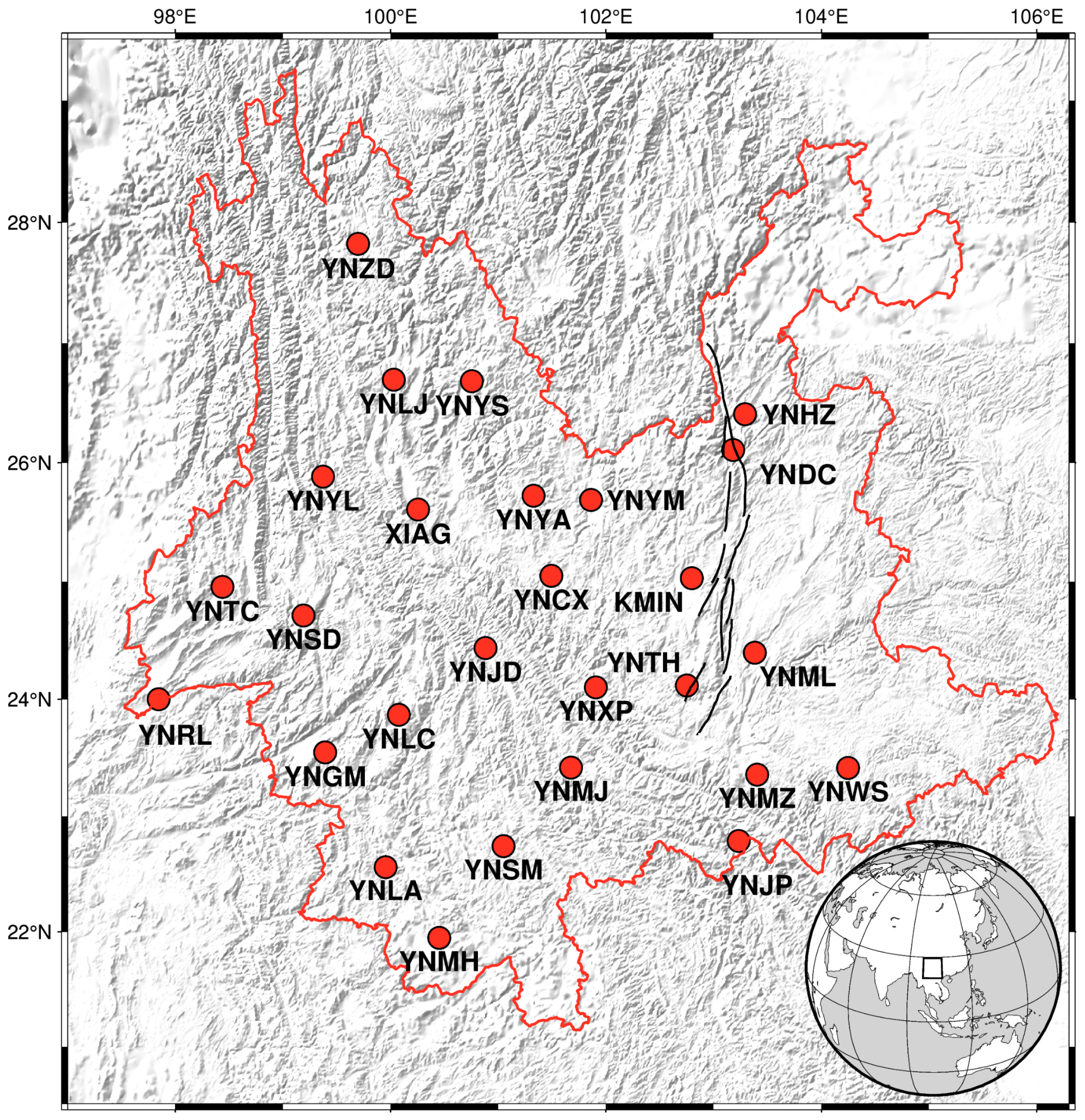
2.1.1. GPS Data
2.1.2. Environmental Loading Model
2.2. Methods
2.2.1. Quantitative Evaluation Metrics
2.2.2. Cross Wavelet Transform
3. Results
3.1. Quantitative Assessment of Environmental Loading Effects
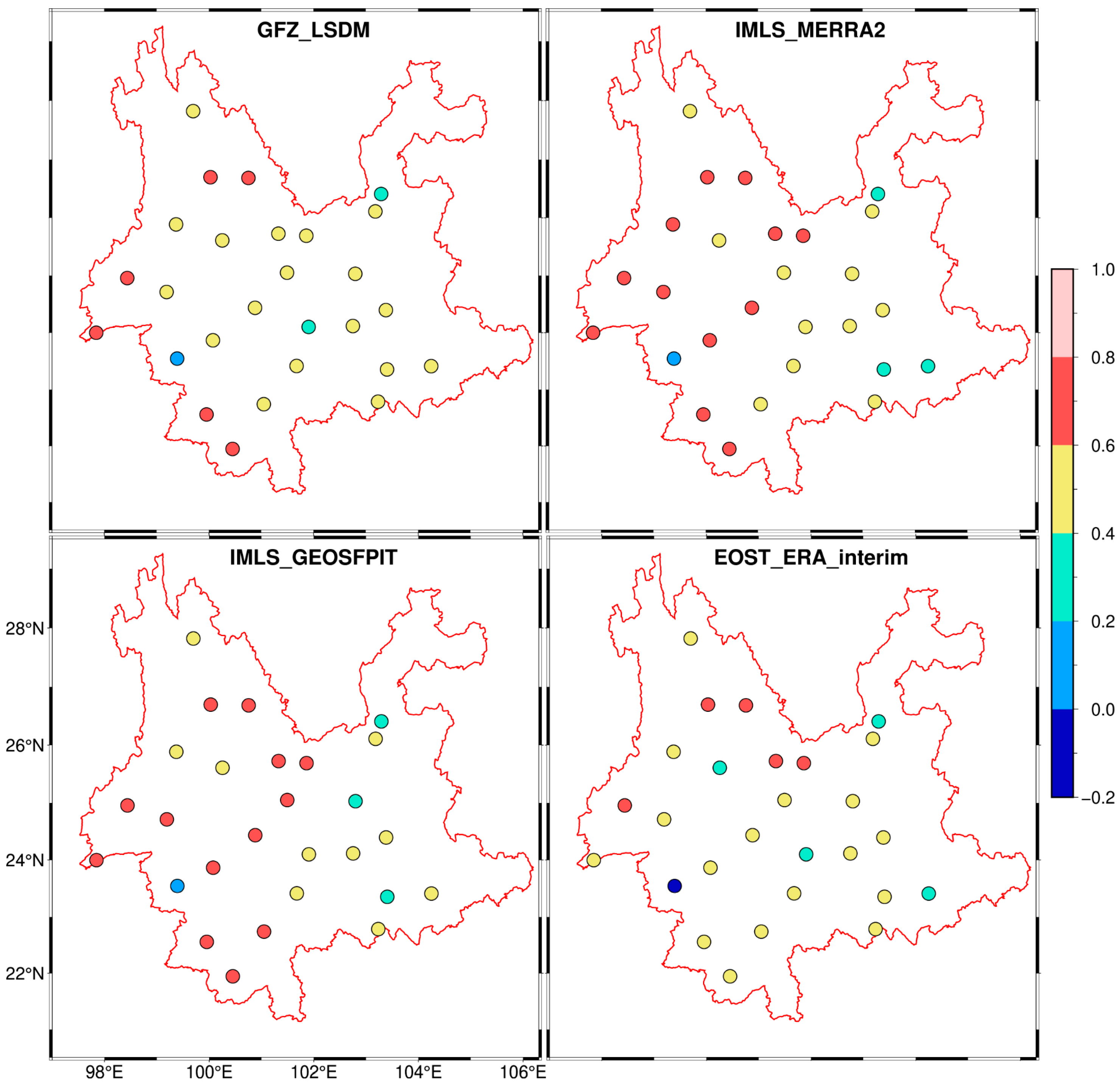
3.1.1. HYDL Effects
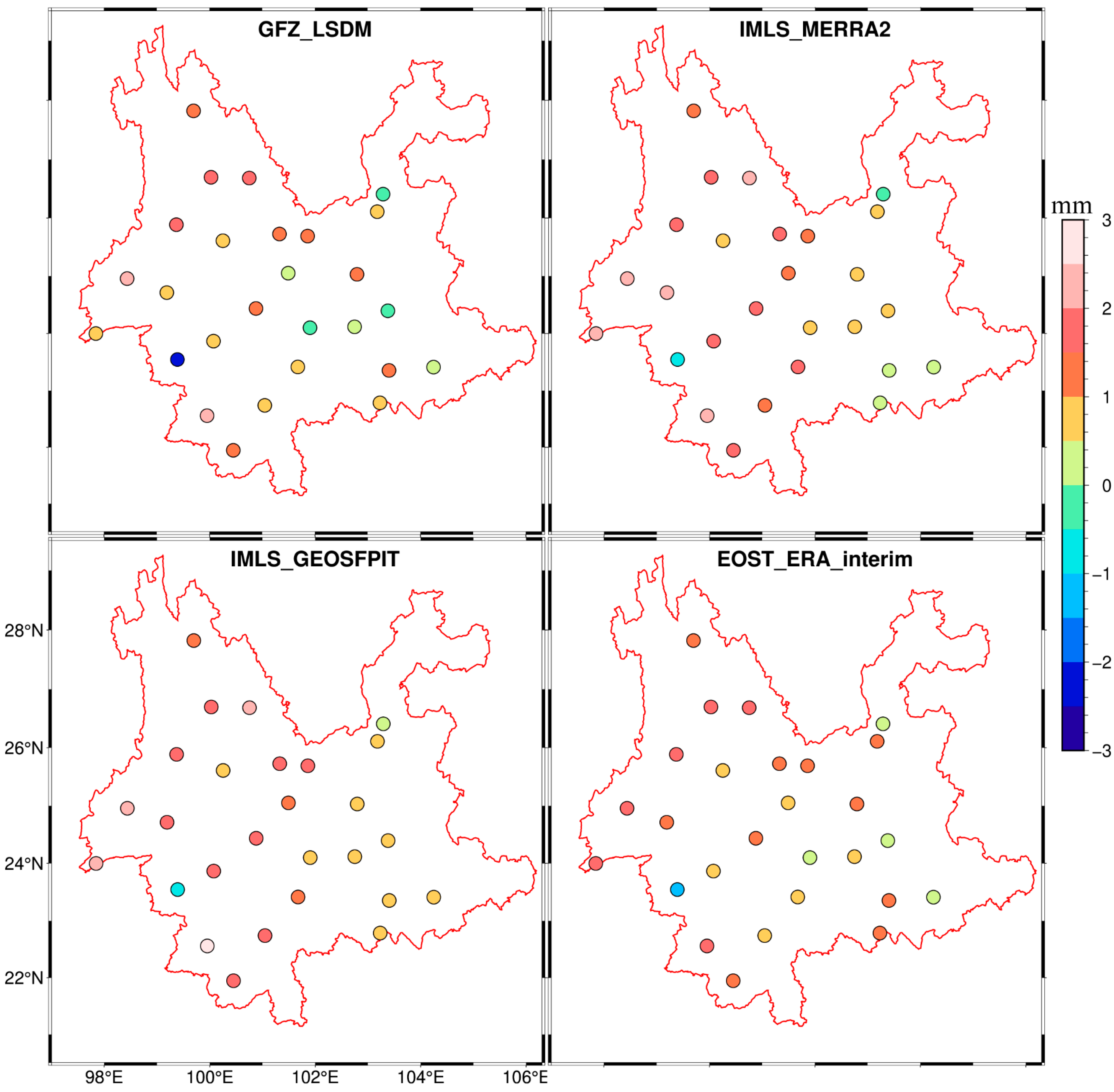
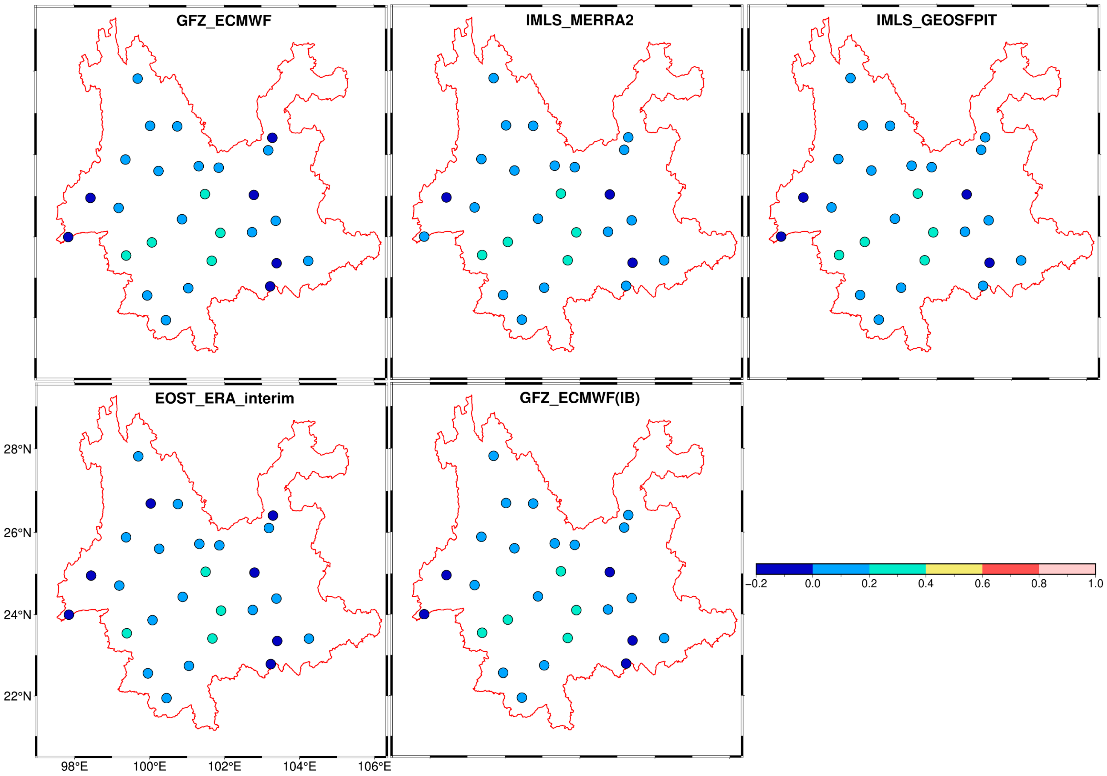
3.1.2. ATML Effects
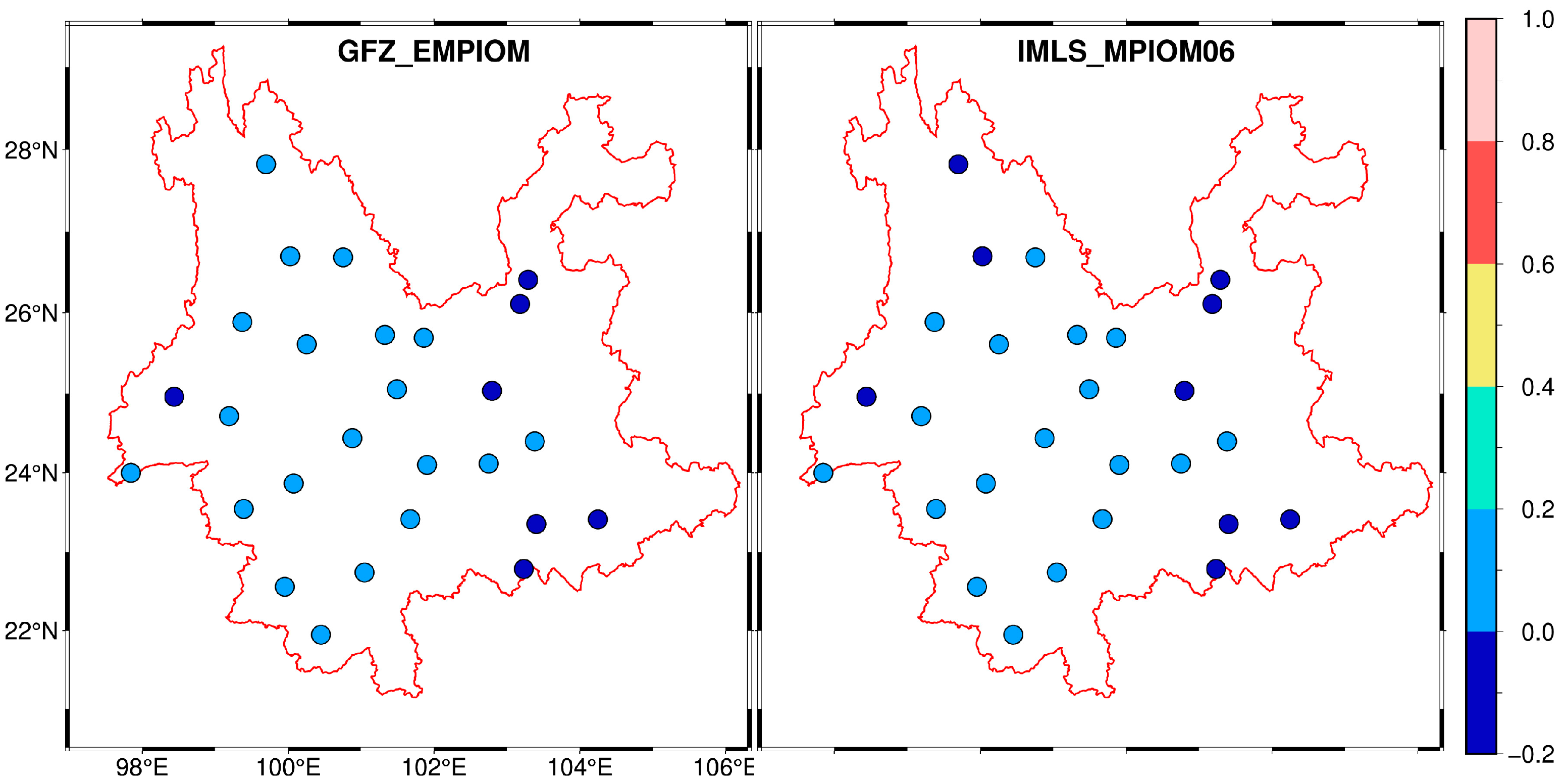
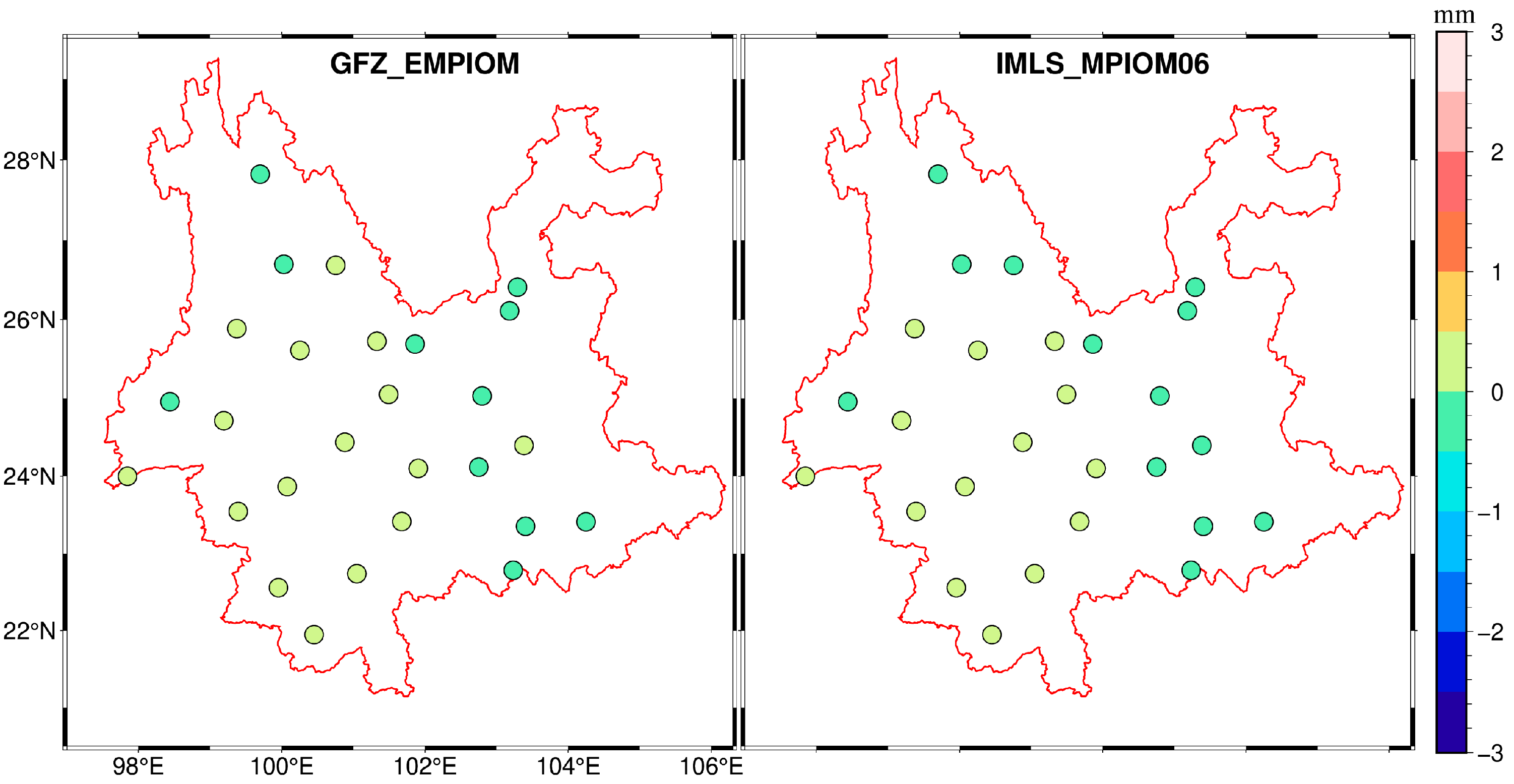
3.1.3. NTOL Effects
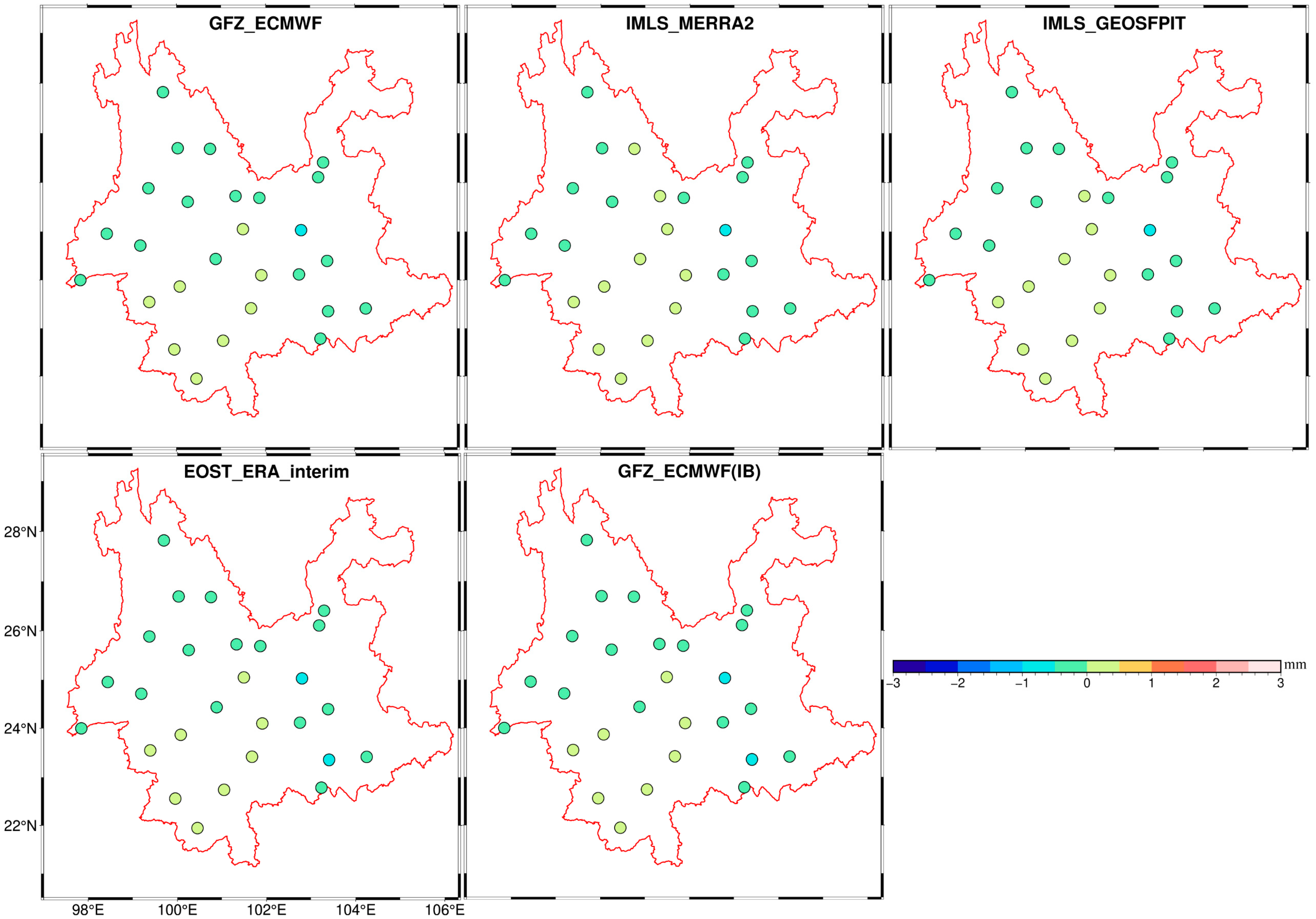
3.1.4. Optimal Combination of HYDL, ATML, and NTOL Effects
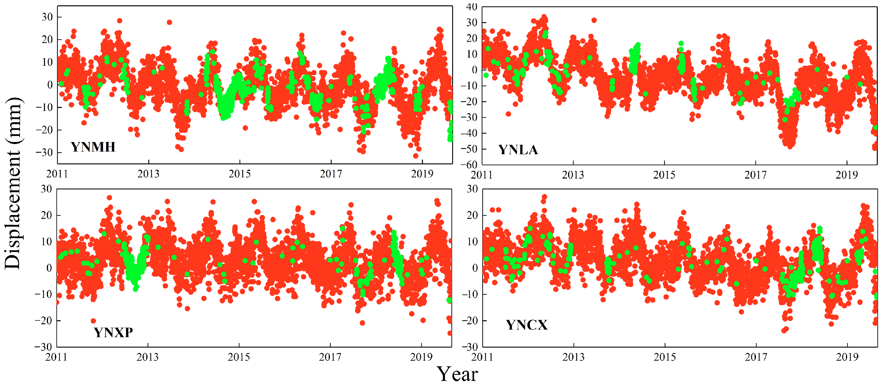
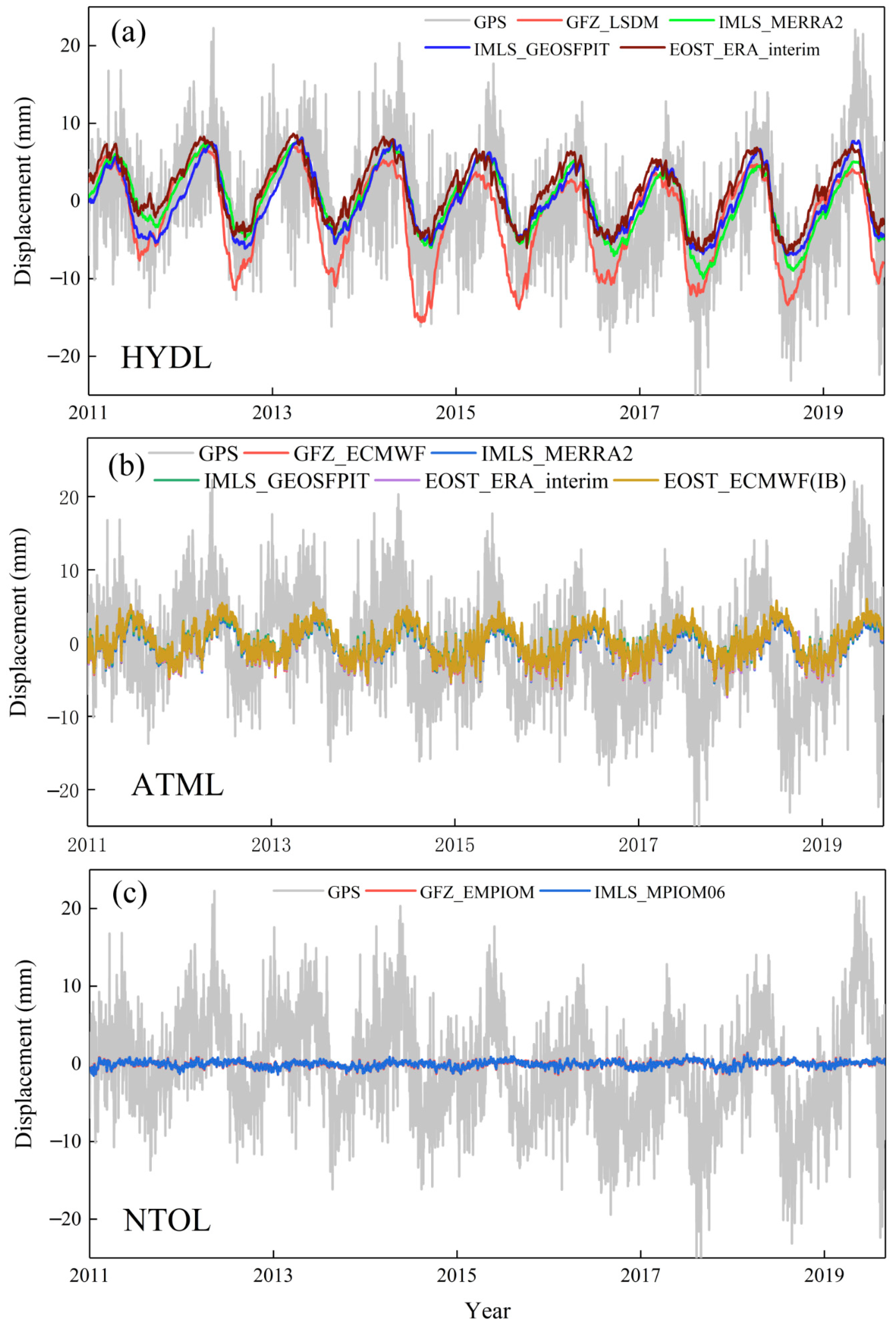
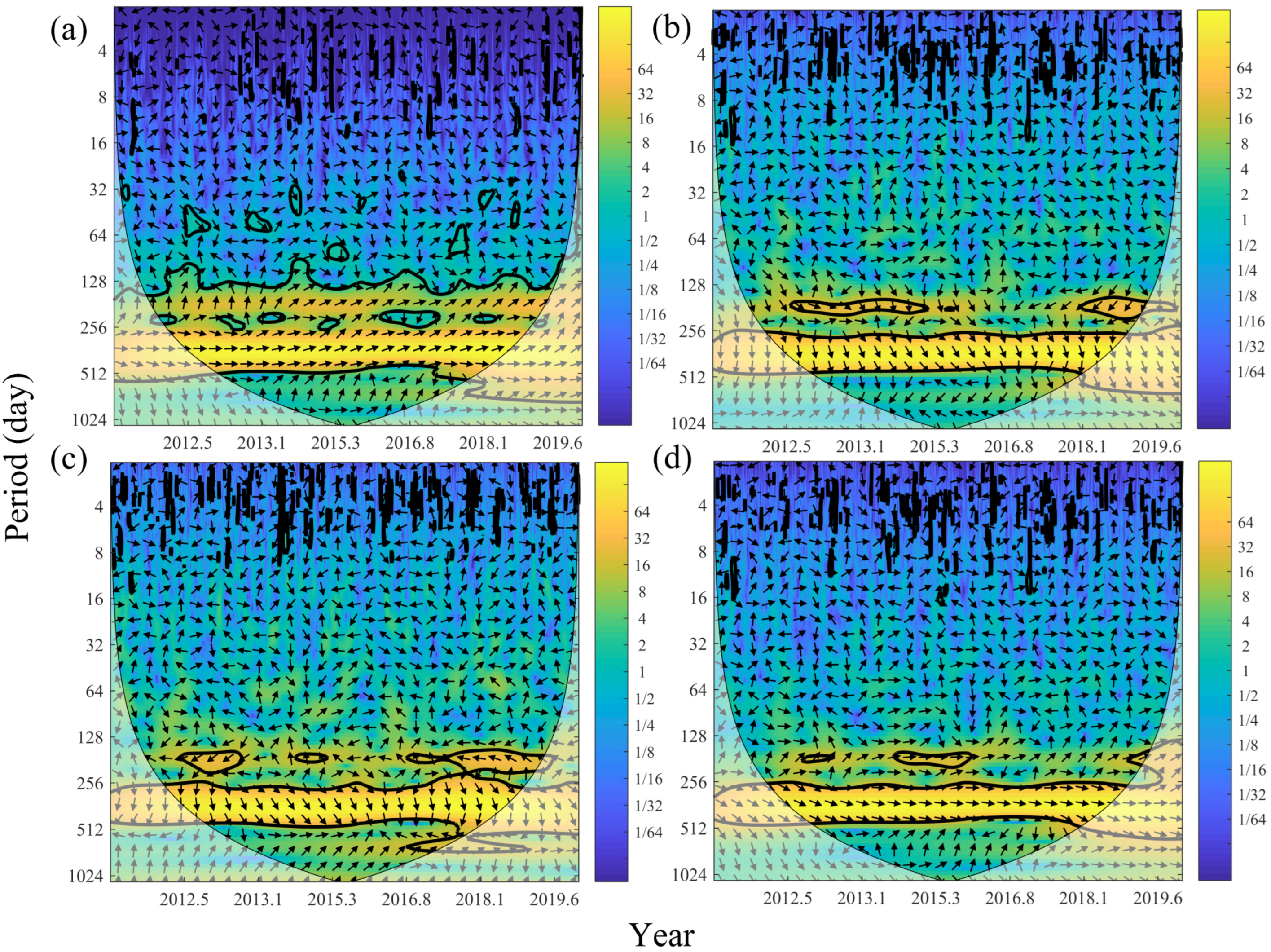
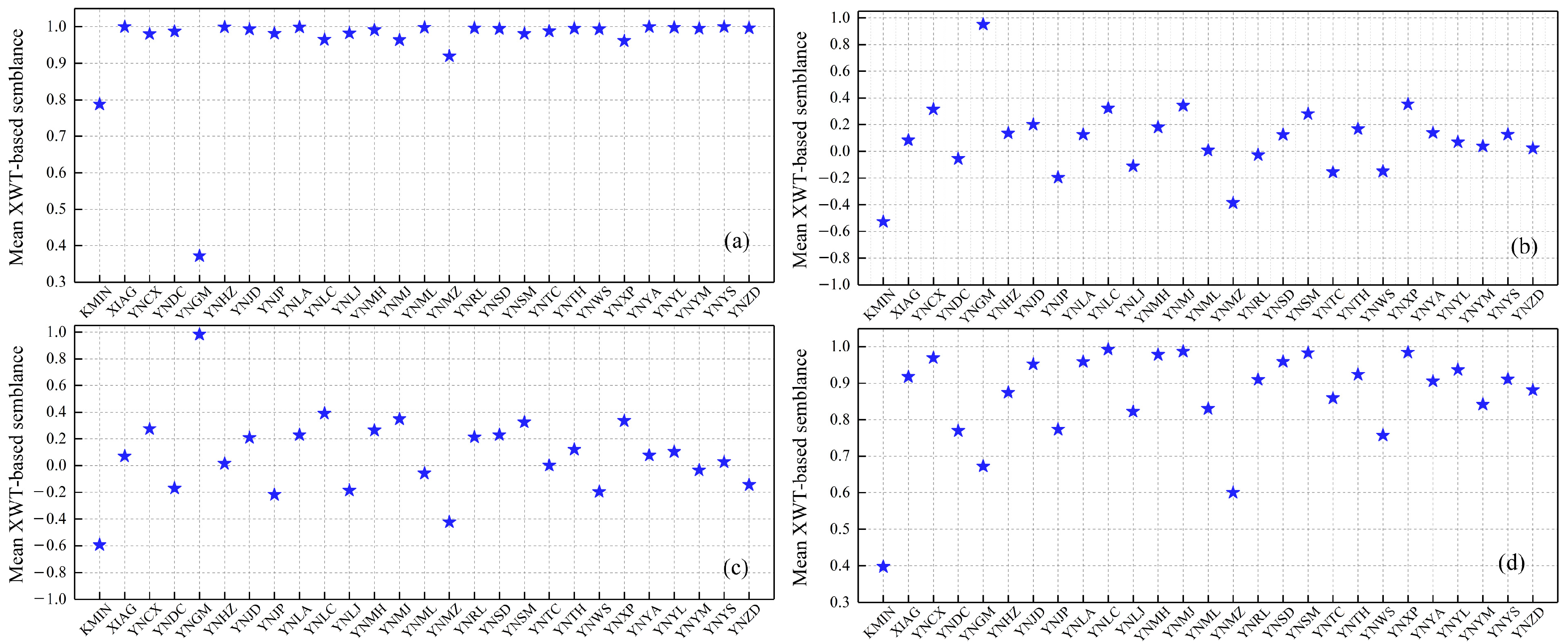
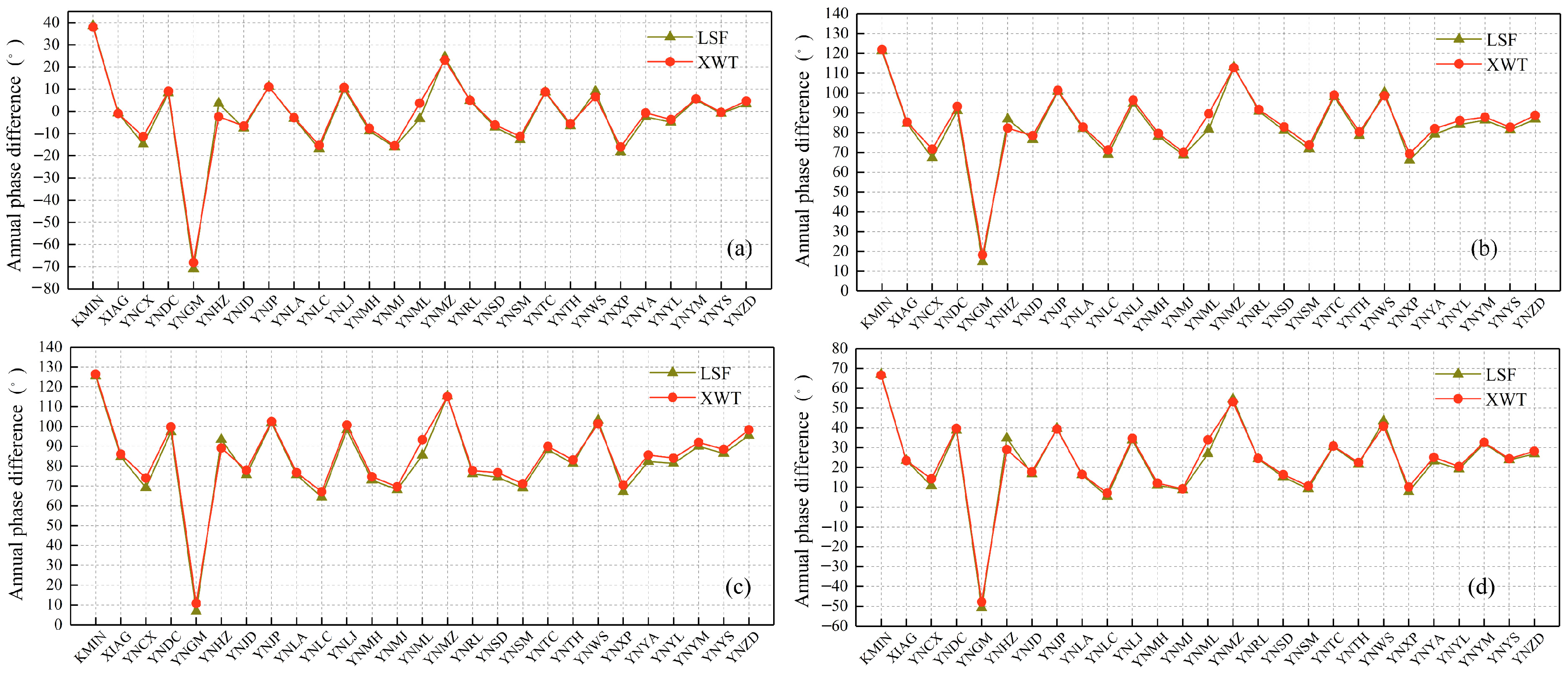
3.2. Cross Wavelet Transform Analysis
4. Discussion
4.1. Changes in the Vertical GPS Time Series Due to Environmental Loading
4.2. The Effects Factors of Vertical GPS Time Series on the Seasonal Variations in Yunnan
5. Conclusions
Author Contributions
Funding
Data Availability Statement
Acknowledgments
Conflicts of Interest
References
- Le Mével, H.; Feigl, K.L.; Córdova, L.; DeMets, C.; Lundgren, P.J. Evolution of unrest at Laguna del Maule volcanic field (Chile) from InSAR and GPS measurements, 2003 to 2014. Geophys. Res. Lett. 2015, 42, 6590–6598. [Google Scholar] [CrossRef]
- Pan, Y.; Hammond, W.C.; Ding, H.; Mallick, R.; Jiang, W.; Xu, X.; Shum, C.; Shen, W.J.J. GPS Imaging of Vertical Bedrock Displacements: Quantification of Two-Dimensional Vertical Crustal Deformation in China. J. Geophys. Res. Solid Earth 2021, 126, e2020JB020951. [Google Scholar] [CrossRef]
- Wang, W.; Qiao, X.; Yang, S.; Wang, D.J. Present-day velocity field and block kinematics of Tibetan Plateau from GPS measurements. Geophys. J. Int. 2017, 208, 1088–1102. [Google Scholar] [CrossRef]
- Kreemer, C.; Blewitt, G.J.J. Robust estimation of spatially varying common-mode components in GPS time-series. J. Geod. 2021, 95, 1–19. [Google Scholar] [CrossRef]
- Li, Z.; Chen, W.; van Dam, T.; Rebischung, P.; Altamimi, Z.J.J. Comparative analysis of different atmospheric surface pressure models and their impacts on daily ITRF2014 GNSS residual time series. J. Geod. 2020, 94, 1–20. [Google Scholar] [CrossRef]
- Nicolas, J.; Verdun, J.; Boy, J.-P.; Bonhomme, L.; Asri, A.; Corbeau, A.; Berthier, A.; Durand, F.; Clarke, P.J. Improved Hydrological Loading Models in South America: Analysis of GPS Displacements Using M-SSA. Remote Sens. 2021, 13, 1605. [Google Scholar] [CrossRef]
- Vandam, T.M.; Blewitt, G.; Heflin, M.B. Atmospheric pressure loading effects on Global Positioning System coordinate determinations. J. Geophys. Res. Solid Earth 1994, 99, 23939–23950. [Google Scholar] [CrossRef]
- Williams, S.; Penna, N.J. Non-tidal ocean loading effects on geodetic GPS heights. Geophys. Res. Lett. 2011, 38. [Google Scholar] [CrossRef] [Green Version]
- Wu, Y.; Zhao, Q.; Zhang, B.; Wu, W.J. Characterizing the seasonal crustal motion in Tianshan area using GPS, GRACE and surface loading models. Remote Sens. 2017, 9, 1303. [Google Scholar] [CrossRef] [Green Version]
- Xiang, Y.; Yue, J.; Li, Z.J.A. Joint analysis of seasonal oscillations derived from GPS observations and hydrological loading for mainland China. Adv. Space Res. 2018, 62, 3148–3161. [Google Scholar] [CrossRef]
- Li, C.; Huang, S.; Chen, Q.; Dam, T.V.; Fok, H.S.; Zhao, Q.; Wu, W.; Wang, X.J. Quantitative evaluation of environmental loading induced displacement products for correcting GNSS time series in CMONOC. Remote Sens. 2020, 12, 594. [Google Scholar] [CrossRef] [Green Version]
- Yuan, P.; Li, Z.; Jiang, W.; Ma, Y.; Chen, W.; Sneeuw, N.J. Influences of environmental loading corrections on the nonlinear variations and velocity uncertainties for the reprocessed global positioning system height time series of the crustal movement observation network of China. Remote Sens. 2018, 10, 958. [Google Scholar] [CrossRef] [Green Version]
- Farrell, W.E. Deformation of the Earth by surface loads. Rev. Geophys. 1972, 10, 761–797. [Google Scholar] [CrossRef]
- Wu, S.; Nie, G.; Meng, X.; Liu, J.; He, Y.; Xue, C.; Li, H. Comparative Analysis of the Effect of the Loading Series from GFZ and EOST on Long-Term GPS Height Time Series. Remote Sens. 2020, 12, 2822. [Google Scholar] [CrossRef]
- Andrei, C.-O.; Lahtinen, S.; Nordman, M.; Näränen, J.; Koivula, H.; Poutanen, M.; Hyyppä, J.J. GPS time series analysis from aboa the finnish antarctic research station. Remote Sens. 2018, 10, 1937. [Google Scholar] [CrossRef] [Green Version]
- Liang, S.; Gan, W.; Shen, C.; Xiao, G.; Liu, J.; Chen, W.; Ding, X.; Zhou, D.J. Three-dimensional velocity field of present-day crustal motion of the Tibetan Plateau derived from GPS measurements. J. Geophys. Res. Solid Earth 2013, 118, 5722–5732. [Google Scholar] [CrossRef]
- Hao, M.; Freymueller, J.T.; Wang, Q.; Cui, D.; Qin, S. Vertical crustal movement around the southeastern Tibetan Plateau constrained by GPS and GRACE data. Earth Planet. Sci. Lett. 2016, 437, 1–8. [Google Scholar] [CrossRef]
- Sheng, C.-Z.; Gan, W.-J.; Liang, S.-M.; Chen, W.-T.; Xiao, G.-R. Identification and elimination of non-tectonic crustal deformation caused by land water from GPS time series in the western Yunnan province based on GRACE observations. Chin. J. Geophys. 2014, 57, 42–52. [Google Scholar]
- Zhan, W.; Li, F.; Hao, W.; Yan, J. Regional characteristics and influencing factors of seasonal vertical crustal motions in Yunnan, China. Geophys. J. Int. 2017, 210, 1295–1304. [Google Scholar] [CrossRef]
- Tan, W.; Dong, D.; Chen, J.J. Application of independent component analysis to GPS position time series in Yunnan Province, southwest of China. Adv. Space Res. 2022, 69, 4111–4122. [Google Scholar] [CrossRef]
- Zhang, K.; Wang, Y.; Gan, W.; Liang, S.J. Impacts of Local Effects and Surface Loads on the Common Mode Error Filtering in Continuous GPS Measurements in the Northwest of Yunnan Province, China. Sensors 2020, 20, 5408. [Google Scholar] [CrossRef] [PubMed]
- Liu, B.; Yu, W.; Dai, W.; Xing, X.; Kuang, C.J. Estimation of Terrestrial Water Storage Variations in Sichuan-Yunnan Region from GPS Observations Using Independent Component Analysis. Remote Sens. 2022, 14, 282. [Google Scholar] [CrossRef]
- Zhan, W. Study on Vertical Crustal Motion in Chinese Mainland and Typical Areas Based on Continuous GPS. Wuhan Wuhan Univ. 2017, 210, 1295–1304. [Google Scholar]
- Li, Y.J. Analysis of GAMIT/GLOBK in high-precision GNSS data processing for crustal deformation. Earthq. Res. Adv. 2021, 1, 100028. [Google Scholar] [CrossRef]
- Zhao, B.; Huang, Y.; Zhang, C.; Wang, W.; Tan, K.; Du, R. Crustal deformation on the Chinese mainland during 1998–2014 based on GPS data. Geod. Geodyn. 2015, 6, 7–15. [Google Scholar] [CrossRef] [Green Version]
- Schneider, T. Analysis of incomplete climate data: Estimation of mean values and covariance matrices and imputation of missing values. J. Clim. 2001, 14, 853–871. [Google Scholar] [CrossRef]
- Hu, S.; Wang, T.; Guan, Y.; Yang, Z.J. Analyzing the seasonal fluctuation and vertical deformation in Yunnan province based on GPS measurement and hydrological loading model. Chin. J. Geophys. Chin. Ed. 2021, 64, 2613–2630. [Google Scholar]
- Li, W.; Li, F.; Zhang, S.; Lei, J.; Zhang, Q.; Yuan, L.J. Spatiotemporal filtering and noise analysis for regional GNSS network in Antarctica using independent component analysis. Remote Sens. 2019, 11, 386. [Google Scholar] [CrossRef] [Green Version]
- Liu, R.; Li, J.; Fok, H.S.; Shum, C.; Li, Z.J.S. Earth surface deformation in the north China plain detected by joint analysis of GRACE and GPS data. Sensors 2014, 14, 19861–19876. [Google Scholar] [CrossRef] [Green Version]
- Dill, R.; Dobslaw, H.J. Numerical simulations of global-scale high-resolution hydrological crustal deformations. J. Geophys. Res. Solid Earth 2013, 118, 5008–5017. [Google Scholar] [CrossRef]
- Dill, R. Hydrological Model LSDM for Operational Earth Rotation and Gravity Field Variations; Scientific Technical Report STR08/09; GFZ German Research Centre For Geosciences: Potsdam, Germany, 2008. [Google Scholar]
- Marsland, S.J.; Haak, H.; Jungclaus, J.H.; Latif, M.; Röske, F.J. The Max-Planck-Institute global ocean/sea ice model with orthogonal curvilinear coordinates. Ocean Model. 2003, 5, 91–127. [Google Scholar] [CrossRef] [Green Version]
- Berrisford, P.; Dee, D.; Fielding, K.; Fuentes, M.; Kallberg, P.; Kobayashi, S.; Uppala, S.J. The ERA-interim archive. ERA Rep. Ser. 2009, 1, 1–16. [Google Scholar]
- Reichle, R.H.; Draper, C.S.; Liu, Q.; Girotto, M.; Mahanama, S.P.; Koster, R.D.; De Lannoy, G.J. Assessment of MERRA-2 land surface hydrology estimates. J. Clim. 2017, 30, 2937–2960. [Google Scholar] [CrossRef] [Green Version]
- Gu, Y.; Yuan, L.; Fan, D.; You, W.; Su, Y.J. Seasonal crustal vertical deformation induced by environmental mass loading in mainland China derived from GPS, GRACE and surface loading models. Adv. Space Res. 2017, 59, 88–102. [Google Scholar] [CrossRef]
- Grinsted, A.; Moore, J.C.; Jevrejeva, S.J. Application of the cross wavelet transform and wavelet coherence to geophysical time series. Nonlinear Processes Geophys. 2004, 11, 561–566. [Google Scholar] [CrossRef]
- Cooper, G.; Cowan, D.J.C. Geosciences. Comparing time series using wavelet-based semblance analysis. Comput. Geosci. 2008, 34, 95–102. [Google Scholar] [CrossRef]
- Peng, Y.; Scales, W.A.; Hartinger, M.D.; Xu, Z.; Coyle, S.J.S.N. Characterization of multi-scale ionospheric irregularities using ground-based and space-based GNSS observations. Satellite Navigation 2021, 2, 1–21. [Google Scholar] [CrossRef]
- Yang, F.; Meng, X.; Guo, J.; Yuan, D.; Chen, M.J.S.N. Development and evaluation of the refined zenith tropospheric delay (ZTD) models. Satellite Navigation 2021, 2, 1–9. [Google Scholar] [CrossRef]
- Bos, M.; Fernandes, R.; Williams, S.; Bastos, L.J. Fast error analysis of continuous GNSS observations with missing data. J. Geod. 2013, 87, 351–360. [Google Scholar] [CrossRef] [Green Version]
- He, X.; Bos, M.S.; Montillet, J.-P.; Fernandes, R.; Melbourne, T.; Jiang, W.; Li, W.J. Spatial Variations of Stochastic Noise Properties in GPS Time Series. Remote Sens. 2021, 13, 4534. [Google Scholar] [CrossRef]
- He, X.; Bos, M.; Montillet, J.; Fernandes, R.J. Investigation of the noise properties at low frequencies in long GNSS time series. J. Geod. 2019, 93, 1271–1282. [Google Scholar] [CrossRef]
- Williams, S.D.; Bock, Y.; Fang, P.; Jamason, P.; Nikolaidis, R.M.; Prawirodirdjo, L.; Miller, M.; Johnson, D.J. Error analysis of continuous GPS position time series. J. Geophys. Res. Solid Earth 2004, 109. [Google Scholar] [CrossRef] [Green Version]
- Yan, H.M.; Chen, W.; ZHU, Y.Z.; ZHANG, W.M.; Zhong, M.; Liu, G.Y. Thermal effects on vertical displacement of GPS stations in China. Chin. J. Geophys. 2010, 53, 252–260. [Google Scholar] [CrossRef]


| Organizations | Type | Model | Spatiotemporal Resolution | Time Span |
|---|---|---|---|---|
| GFZ | HYDL | LSDM | 0.5° × 0.5°/24 h | 1976–present |
| ATML | ECMWF | 0.5° × 0.5°/3 h | ||
| NTOL | EMPIOM | 1° × 1°/3 h | ||
| IMLS | HYDL | MERRA2 | 2′ × 2′/3 h | 1980–present |
| HYDL | GEOSFPIT | 2′ × 2′/3 h | 2000–present | |
| ATML | MERRA2 | 2′ × 2′/6 h | 1980–present | |
| ATML | GEOSFPIT | 2′ × 2′/3 h | 2000–present | |
| NTOL | MPIOM06 | 2′ × 2′/3 h | 1980–present | |
| EOST | HYDL | ERA interim | 0.5° × 0.5°/6 h | 1979–2019 |
| ATML | ERA interim | 0.5° × 0.5°/6 h | ||
| ATML | ECMWF(IB) | 0.5° × 0.5°/3 h | 2000–present |
| Combination | Correlation | RMS Reduction (mm) | ||
|---|---|---|---|---|
| HYDL | ATML | NTOL | ||
| GFZ_LSDM | EOST_ERA_interim | IMLS_MPIOM06 | 0.57 | 1.24 |
| GFZ_LSDM | EOST_ECMWF(IB) | IMLS_MPIOM06 | 0.57 | 1.24 |
| GFZ_LSDM | EOST_ERA_interim | GFZ_EMPIOM | 0.57 | 1.24 |
| GFZ_LSDM | EOST_ECMWF(IB) | GFZ_EMPIOM | 0.57 | 1.23 |
| GFZ_LSDM | GFZ_ECMWF | IMLS_MPIOM06 | 0.57 | 1.23 |
| GFZ_LSDM | IMLS_GEOSFPIT | IMLS_MPIOM06 | 0.57 | 1.23 |
| GFZ_LSDM | EOST_ERA_interim | GFZ_EMPIOM | 0.57 | 1.23 |
| GFZ_LSDM | EOST_ERA_interim | GFZ_EMPIOM | 0.57 | 1.22 |
| EOST_ERA_interim | EOST_ERA_interim | GFZ_EMPIOM | 0.53 | 1.22 |
| EOST_ERA_interim | IMLS_MERRA2 | IMLS_MPIOM06 | 0.53 | 1.22 |
| IMLS_MERRA2 | IMLS_MERRA2 | GFZ_EMPIOM | 0.51 | 1.00 |
| IMLS_MERRA2 | IMLS_MERRA2 | IMLS_MPIOM06 | 0.51 | 0.99 |
| IMLS_MERRA2 | IMLS_GEOSFPIT | GFZ_EMPIOM | 0.51 | 0.99 |
| IMLS_MERRA2 | IMLS_GEOSFPIT | IMLS_MPIOM06 | 0.51 | 0.98 |
| IMLS_MERRA2 | EOST_ECMWF(IB) | GFZ_EMPIOM | 0.51 | 0.93 |
| IMLS_MERRA2 | GFZ_ECMWF | IMLS_MPIOM06 | 0.51 | 0.93 |
| IMLS_MERRA2 | EOST_ECMWF(IB) | IMLS_MPIOM06 | 0.50 | 0.92 |
| IMLS_MERRA2 | GFZ_ECMWF | IMLS_MPIOM06 | 0.50 | 0.92 |
| IMLS_MERRA2 | EOST_ERA_interim | GFZ_EMPIOM | 0.50 | 0.92 |
| IMLS_MERRA2 | EOST_ERA_interim | IMLS_MPIOM06 | 0.50 | 0.91 |
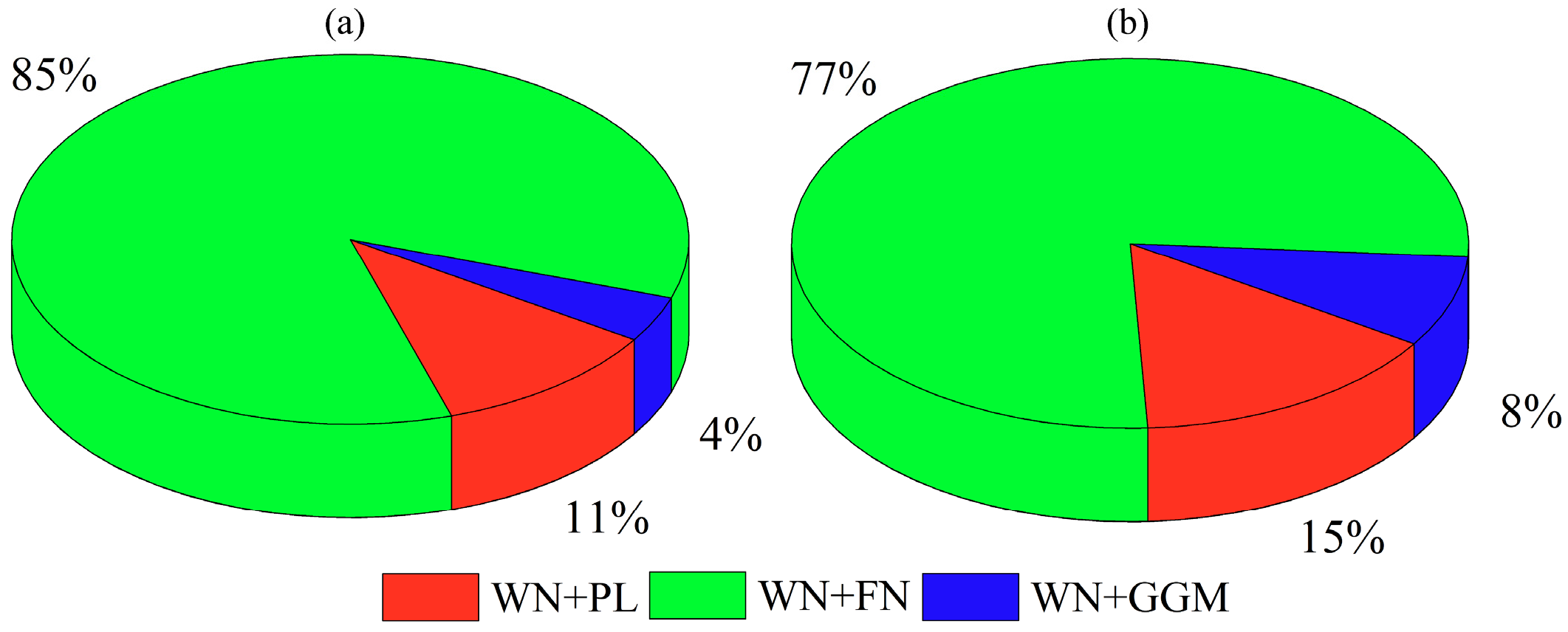
| Stations | Before Correction | After Correction | Stations | Before Correction | After Correction |
|---|---|---|---|---|---|
| KMIN | WN + PL | WN + PL | YNMZ | WN + FN | WN + FN |
| XIAG | WN + FN | WN + FN | YNRL | WN + FN | WN + FN |
| YNCX | WN + FN | WN + FN | YNSD | WN + FN | WN + GGM |
| YNDC | WN + FN | WN + FN | YNSM | WN + FN | WN + PL |
| YNHZ | WN + FN | WN + FN | YNTC | WN + FN | WN + FN |
| YNJD | WN + FN | WN + FN | YNTH | WN + FN | WN + PL |
| YNJP | WN + FN | WN + FN | YNWS | WN + FN | WN + FN |
| YNLA | WN + PL | WN + FN | YNXP | WN + FN | WN + FN |
| YNLC | WN + FN | WN + FN | YNYA | WN + FN | WN + FN |
| YNLJ | WN + FN | WN + FN | YNYL | WN + FN | WN + FN |
| YNMH | WN + FN | WN + FN | YNYM | WN + FN | WN + FN |
| YNMJ | WN + FN | WN + FN | YNYS | WN + GGM | WN + GGM |
| YNML | WN + FN | WN + FN | YNZD | WN + PL | WN + PL |
Publisher’s Note: MDPI stays neutral with regard to jurisdictional claims in published maps and institutional affiliations. |
© 2022 by the authors. Licensee MDPI, Basel, Switzerland. This article is an open access article distributed under the terms and conditions of the Creative Commons Attribution (CC BY) license (https://creativecommons.org/licenses/by/4.0/).
Share and Cite
Hu, S.; Chen, K.; Zhu, H.; Xue, C.; Wang, T.; Yang, Z.; Zhao, Q. A Comprehensive Analysis of Environmental Loading Effects on Vertical GPS Time Series in Yunnan, Southwest China. Remote Sens. 2022, 14, 2741. https://doi.org/10.3390/rs14122741
Hu S, Chen K, Zhu H, Xue C, Wang T, Yang Z, Zhao Q. A Comprehensive Analysis of Environmental Loading Effects on Vertical GPS Time Series in Yunnan, Southwest China. Remote Sensing. 2022; 14(12):2741. https://doi.org/10.3390/rs14122741
Chicago/Turabian StyleHu, Shunqiang, Kejie Chen, Hai Zhu, Changhu Xue, Tan Wang, Zhenyu Yang, and Qian Zhao. 2022. "A Comprehensive Analysis of Environmental Loading Effects on Vertical GPS Time Series in Yunnan, Southwest China" Remote Sensing 14, no. 12: 2741. https://doi.org/10.3390/rs14122741
APA StyleHu, S., Chen, K., Zhu, H., Xue, C., Wang, T., Yang, Z., & Zhao, Q. (2022). A Comprehensive Analysis of Environmental Loading Effects on Vertical GPS Time Series in Yunnan, Southwest China. Remote Sensing, 14(12), 2741. https://doi.org/10.3390/rs14122741