Abstract
The use of the conventional interferometric synthetic aperture radar (InSAR) to generate digital elevation models (DEMs) always encounters phase unwrapping (PU) errors in areas with a sizeable topographic gradient. Range split-spectrum interferometry (RSSI) can overcome this issue; however, it loses the spatial resolution of the SAR image. We propose the use of the RSSI-assisted In-SAR-derived DEM (RID) method to address this challenge. The proposed approach first applies the RSSI method to generate a prior DEM, used for simulating terrain phases. Then, the simulated terrain phases are subtracted from the wrapped InSAR phases to obtain wrapped residual phases. Finally, the residual phases are unwrapped by the minimum cost flow (MCF) method, and the unwrapped residual phases are added to the simulated phases. Both the simulated and TerraSAR-X data sets are used to verify the proposed method. Compared with the InSAR and RSSI methods, the proposed approach can effectively decrease the PU errors of large gradients, ensure data resolution, and guarantee the DEM’s accuracy. The root mean square error between the topographic phase simulated from the real DEM and the topographic phase generated from the proposed method is 2.22 rad, which is significantly lower than 6.60 rad for InSAR, and the improvement rate is about 66.36%.
1. Introduction
The digital elevation model (DEM) describes ground elevation information, which plays an important role in the national economy and defense construction. DEM can be generated by optical stereo image pairs, LiDAR, and traditional measurement methods [1,2,3,4]. However, these are either highly affected by clouds, rain, and fog, or extremely inefficient and costly. Interferometric synthetic aperture radar (InSAR) is extensively used to generate DEM because it can effectively overcome the defects mentioned above [5,6]. Unfortunately, phase unwrapping (PU) is an essential step for InSAR DEM extraction, which can directly affect the DEM quality [7]. For regions with a large topographic gradient, the phase fringes of InSAR-derived DEM are extremely dense. Therefore, it is easy to cause phase unwrapping errors and thus seriously affect the quality of InSAR-derived DEM. Several PU methods exist to address the problem of InSAR phase unwrapping. The most common PU methods include: (1) single-baseline PU (SB-PU) method and (2) multibaseline PU (MB-PU) method [8,9,10,11]. The SB-PU method can quickly retrieve the unwrapping phase based on the phase continuity assumption, which was first proposed by Itoh [12]. This assumption works in the scenario where the phase difference between any two adjacent pixels is less than π [7,13]. The SB-PU method mainly includes the path-following methods (e.g., the branch-cut method), optimization-based methods (e.g., minimum cost flow method, MCF; SNAPHU method), and integrated denoising and unwrapping methods (e.g., Kalman-filter-based PU method) [8,14,15,16,17,18,19]. Nevertheless, the phase continuity assumption is not always true, especially in scenes with large gradient deformation and topographic changes. Therefore, the unwrapping performance of the SB-PU method for InSAR-derived DEM phases of areas with large topographic gradients is vastly reduced. In contrast to the SB-PU method, the MB-PU method uses more InSAR interferometric pairs and significantly increases the ambiguity intervals of interferometric phases, effectively overcoming the phase continuity condition [8,13,20]. The MB-PU method mainly consists of parametric-based (e.g., Maximum-likelihood estimation and maximum a posterior estimation), nonparametric-based (Chinese remainder theorem), and cluster-analysis (CA)-based methods [8,21,22,23,24]. Although the MB-PU method can effectively overcome the phase continuity assumption, its implementation is quite difficult, and it suffers from poor robustness and low efficiency.
With the continuous enrichment of external data and the rapid development of data processing technology, on the one hand, the external data-assisted PU method has captured widespread attention, e.g., external DEM-assisted methods [25,26]. Unfortunately, the effectiveness of this method depends heavily on the accuracy and immediacy of external data, e.g., the external DEM is too old to reflect the real surface information. Moreover, the performance of the external DEM-assisted PU method will be significantly reduced. On the other hand, the deep learning technique has presented powerful performances in terms of detecting, segmentation, and recognizing objects with optical images [27,28,29]. Recently, a few studies have revealed that the deep learning technique has immense potential in InSAR phase unwrapping and can effectively overcome phase unwrapping errors [30,31,32,33,34,35,36,37,38]. However, the number and diversity of samples struggle to meet the actual situation. Additionally, the InSAR phase unwrapping model of deep learning is limited by its generalization ability, which leads to phase-unwrapping distortion in complex scenes.
Although the PU methods mentioned above can effectively reduce the unwrapping errors of InSAR-derived DEM in some scenarios, they are limited by the phase continuity assumption, robustness and efficiency, the accuracy and immediacy of external data, or samples and generalization ability. In this context, the range split-spectrum interferometry (RSSI) has gradually caught the attention of the InSAR community in recent years [39]. Several studies have demonstrated that the RSSI method has immense potential to reduce phase unwrapping errors for InSAR-derived DEM [40,41]. The RSSI method uses the split-spectrum technique to generate low- and high-frequency SAR image sub-bands. The SAR sub-bands are then used to form low- and high-frequency interferograms. Finally, the difference between the sub-band interferograms (double differential interferogram) is used to simulate an interferogram with a longer carrier wavelength than that of the SAR system [40]. This simulation can increase the height of ambiguity (HoA) to a pixel where phase unwrapping is unnecessary. Therefore, the apparent advantage of the RSSI method is that the phase unwrapping error can be ignored [40,41]. However, using the RSSI method to simulate an interferogram with a larger carrier wavelength requires multiplying by a scale factor. This factor will amplify the noise in the double differential interferogram. To overcome this problem, a low-pass filter is needed to reduce the variance in the double differential interferogram. Unfortunately, this smoothing process will sacrifice the resolution of the double differential interferogram. Although the RSSI method cannot obtain DEMs with high accuracy, it can assist conventional InSAR in generating DEMs to reduce the influence of phase unwrapping errors.
According to the above statements, this study proposes a method that uses the RSSI method to assist InSAR-derived DEM (RID) in overcoming phase-unwrapping errors. The proposed method first uses the RSSI to simulate a topographic phase. Then, the simulated topographic phase is subtracted from the InSAR phase. Afterward, the residual InSAR phase is unwrapped. Finally, the simulated topographic phase is added to the unwrapped residual InSAR phase and converted to DEM. In contrast to the PU methods mentioned above, conventional InSAR, and RSSI, the proposed method has the following advantages: (1) it does not need a large number of SAR images, the implementation process is simple, and it can guarantee the immediacy of assisted data, (2) it can effectively reduce the phase unwrapping errors of conventional InSAR-derived DEM, and (3) it can vastly compensate the loss of resolution in the RSSI method. To test the proposed method, both the simulated and TerraSAR-X data sets are used. In addition, we used the topographic phase simulated from a Copernicus DEM to validate the proposed method.
2. Methods
InSAR measurements’ high resolution, extensive range, and high accuracy make it a hot technology to generate DEMs. For the InSAR measurement, the relationship between the absolute phase and the terrain height can be expressed as follows:
where a and r represent the coordinates of a pixel, along with its azimuth and range directions, respectively, h(a, r) is the terrain height, c represents the light speed in a vacuum, R(a, r) is the slant range, θ represents the incidence angle, f0 is the radar carrier frequency, represents the perpendicular baseline, and φ0(a, r) represents the absolute phase.
2.1. Basic Principle of the RSSI Method
Equation (1) shows that the terrain height is proportional to the absolute phase and inversely proportional to the radar carrier frequency. Any SAR image with a carrier frequency of f0 can be split into two non-overlapping sub-band SAR images at slightly different carrier frequencies (i.e., high and low frequencies) by the band-pass filter [13,14,15,16]. Therefore, a pair of SAR images can be used to generate four sub-band SAR images, which can be used to form two sub-band interferograms. Equation (1) can thus be rewritten as
where fH and fL represent the carrier frequencies of the high- and low-frequency sub-band SAR images, respectively; φH(a, r) and φL(a, r) represent the high and low frequencies absolute phases, respectively. Equation (2) can calculate the terrain height, i.e.,
where φH-L(a, r)= φH(a, r) − φL(a, r).
2.2. Basic Principle of the RID Method
Since the difference between fH and fL is very small, the difference between φH(a, r) and φL(a, r) is also tiny. This means, on the one hand, that the phase fringes of the wrap (φH-L) are so sparse that it is easy to unwrap, and on the other hand, the robustness of Equation (3) is poor, i.e., a small amount of noise in φH-L(a, r) will significantly affect the accuracy of h(a, r). Therefore, to improve the accuracy of terrain height, several executions of low-pass filter are required for φH-L(a, r) to reduce noise. This filtering process can significantly reduce the result’s resolution, thus losing some terrain information. To rectify this problem, the RSSI-assisted InSAR-derived DEM (RID) method is proposed. This method first uses the RSSI method to obtain the prior terrain height, which is used to simulate an unwrapped terrain phase φRSSI(a, r). Then, φRSSI(a, r) to [−π, π] is rewrapped, i.e., , and is subtracted from the wrapped terrain phase obtained from the conventional InSAR. This process can reduce the phase fringes of the InSAR phase to overcome the phase continuity assumption obeyed by traditional phase unwrapping methods. The residual wrap phase is
Afterward, the MCF method is used to unwrap the residual wrap phase and then add it to φRSSI(a, r). This process can compensate for the loss of the DEM resolution generated from the RSSI method. The last terrain phase can be written as follows
where φRID(a, r) is the terrain phase obtained from the RID method; φresid(a, r) represents the unwrapped residual phase. Substituting φRID(a, r) into Equation (1) can obtain the terrain height,
2.3. Implementation of the RID Method
To implement the proposed method, eight steps are needed, as follows:
Step 1: Generate the sub-band single look complex (SLC) SAR images with high and low carrier frequencies from the primary and secondary SAR images, respectively.
Step 2: Coregister the full-bandwidth SLCs and obtaining the refined coregistration files (e.g., lookup table and polynomial), which are used for the sub-band SLCs’ coregistration.
Step 3: Generate the high- and low-frequency interferograms and the conventional InSAR interferogram.
Step 4: Remove the flat earth phases in the high- and low-frequency interferograms and the conventional InSAR interferogram and use the high- and low-frequency interferograms without a flat earth phase to obtain the double differential interferogram.
Step 5: Convert the double differential phase to the terrain height using Equation (3).
Step 6: Use the terrain height obtained from step 5 and the orbit data of SAR satellite to simulate a terrain phase and subtract it from the conventional InSAR interferogram without a flat earth phase.
Step 7: Unwrap the residual phase obtained in step 6 and add it to the simulated terrain phase from step 6 to generate the last terrain phase.
Step 8: Convert the last terrain phase generated to terrain height using Equation (6). The implementation details of the RID method are shown in Figure 1. The RID method uses the prior terrain height obtained by the RSSI method to circumvent the unwrapping problem in the region with a large terrain gradient and uses the terrain phase extracted by conventional InSAR to ensure the resolution of the generated DEM.
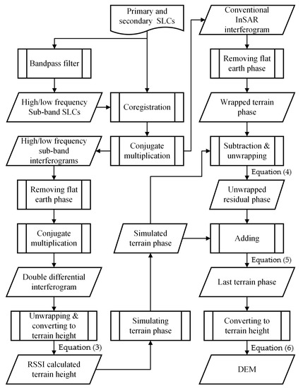
Figure 1.
The implementation flowchart of the RID method.
3. Experimental Results and Analyses
In this study, we used both the simulation data and a pair of TerraSAR-X data on spotlight mode to verify the validity of the RID method. Furthermore, we compared the results generated from the conventional InSAR and RSSI methods with the proposed method. Finally, the accuracy was evaluated by the root mean square error (RMSE) between the results obtained from the three methods mentioned above and that of the reference data. The RMSE can be expressed as follows:
where N is the number of pixels; M represents the different methods, i.e., InSAR, RSSI, or RID; φM represents the terrain phase obtained from InSAR, RSSI, or RID; φr is the reference terrain phase; and i represents the ith pixel.
3.1. Simulated Experiment
To test the performance of the proposed method, we first employed the peaks function to simulate a DEM that the elevations varied from [0, 1000] m, which is shown in Figure 2a. We then used the simulated DEM and a MATLAB toolbox of the simulated InSAR system provided by the Delft University of Technology to generate the InSAR-based DEM phase, shown in Figure 2b. The major parameters used to simulate the InSAR-based DEM are presented in Table 1. Similar to the literature [23], we also took the Gaussian noise using corrected sigma as the phase noise, which accounts for geometric decorrelation. The corrected sigma can be calculated based on coherence and number of looks [23]. Figure 2c shows the simulated phase noise (Gaussian noise), and Figure 2d presents the rewrapped InSAR terrain phases of Figure 2b added Figure 2c.
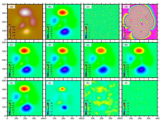
Figure 2.
Performance comparison of the conventional InSAR, RSSI, and RID methods based on the simulated data set: (a) represents the simulated DEM; (b) is the unwrapped phase converted from (a), i.e., full-bandwidth InSAR-based DEM phase; (c) is the Gaussian noise, and (d) is the rewrapped phase of (b) added (c); (e,f) show the simulated noisy high- and low-frequency DEM interferometric phases; (g–i) represent the terrain phase from conventional InSAR, RSSI, and RID methods, respectively; (j–l) present the differences between (b,g–i).

Table 1.
Major Parameters of the Simulated InSAR System.
To obtain the conventional InSAR result, the MCF PU method was used to unwrap the rewrapped terrain phases in Figure 2d, and Figure 2g shows the unwrapped terrain phases. For the implementation of the RSSI method, we first simulated the high- (Figure 2e) and low-frequency (Figure 2f) terrain phases with Gaussian noise and then calculated the terrain phases based on Equations (1)–(4); the simulated result is illustrated in Figure 2h. Note that, according to [42], the accuracy and resolution of the DEM extraction by the RSSI method are relatively ideal when the carrier frequencies of the high- and low-frequency sub-bands are f0 + 0.4B (B is the range bandwidth) and f0 − 0.4B for the TerraSAR-X data with a range bandwidth of 300 MHz, respectively. Therefore, we used the same strategy here to simulate the implementation of the RSSI method. The RID method was implemented following the steps described in Figure 1, and the result is presented in Figure 2i.
Figure 2d shows the simulated data with dense phase fringes, which can be considered the area with large gradient terrain changes. Figure 2j–l illustrate the residual errors between Figure 2b and Figure 2g–i, respectively. Figure 2g,j indicate that DEM extraction using the conventional InSAR encounters serious PU errors in areas with large terrain gradient changes and the maximum residual error reaches about 20 rad. In contrast, the PU problem is trivial for the RSSI and proposed methods. Figure 2h,i revealed that the results of the RSSI and proposed methods are in reasonable agreement with the original simulated data (Figure 2b); the corresponding absolute residual errors are less than 6.5 rad (Figure 2k) and 2.0 rad (Figure 2l), respectively. The results showed that the RMSEs are 2.7666 rad, 1.4885 rad, and 0.3827 rad for conventional InSAR, RSSI, and RID methods. Compared with InSAR and RSSI methods, the RMSE improvement rate of the RID method is 86.17% and 74.29%, respectively. The RMSRE reveals that the accuracy of the RID method is optimal. As illustrated above, the simulation experiments testify to the superiority of the proposed RID method. Nevertheless, Figure 2j–l show that the residual errors for the RSSI and our methods are distributed in the whole region, while those of the conventional InSAR method are mainly distributed in the region with large terrain gradient variation. This is mainly because the RSSI method amplified the noises in the simulated terrain phases. These phenomena also reveal that the RSSI and proposed methods are more sensitive to noise than the conventional InSAR method.
3.2. TerraSAR-X on Spotlight Mode
To further illustrate the performance of the RID method, a pair of TerraSAR-X images in spotlight mode, with a range bandwidth of 300 MHz, were used. This pair of SAR images cover parts of the Uluru-Kata National Park (the white rectangle in Figure 3a), including both flat terrain and the Ayers Rock with a large terrain gradient (Figure 3a,b), which is helpful to adequately verify the applicability of the RID method under different terrain conditions. The major parameters of the SAR image pair are shown in Table 2. Additionally, we selected the Copernicus DEM with a resolution of 30 m to validate the accuracy of the proposed method (Figure 4a). This type of DEM was chosen for validation, mainly because it has been proven to be superior to other similar DEM products (such as ALOS, ASTER, NASA, and SRTM) in high relief, and with different vegetation types and gentle and steep slopes, and the absolute vertical accuracy is below 2 m in some regions of the world [43,44]. The Copernicus DEM was derived from the editing of the WorldDEM™ products, which are based on X-band SAR data acquired by the TanDEM-X mission in the time period 2010–2015; it is, therefore, newer than the other DEM products (such as ALOS, ASTER, NASA, and SRTM) [45].
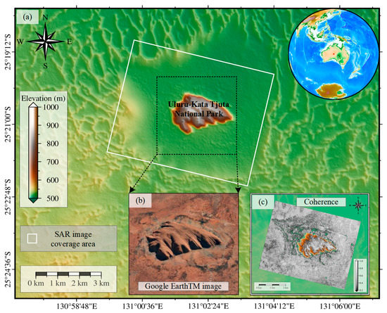
Figure 3.
The study area: (b) represents the google image of the black dotted rectangle in (a), (c) is the coherence of the pair of TerraSAR-X images.
Table 2.
The Major Parameters of The Realistic Sar Image Pair.
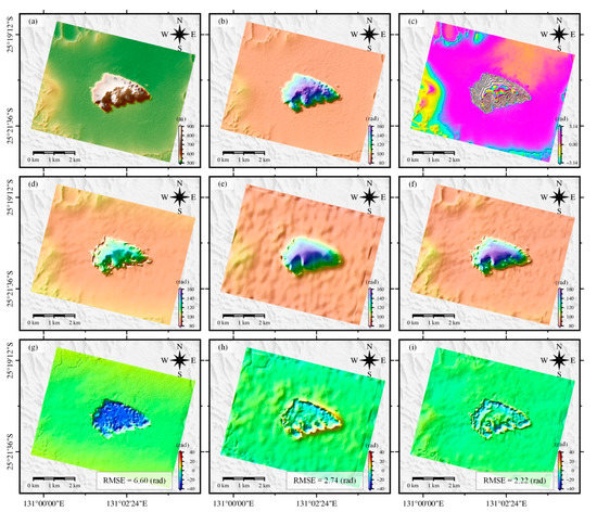
Figure 4.
Performance comparisons of the conventional InSAR, RSSI, and RID methods based on the realistic TerraSAR-X data set: (a–c) represent the Copernicus DEM, unwrapped phase converted from the Copernicus DEM, and rewrapped phase converted from the Unwrapped phase, respectively; (d–f) show the reconstructed DEM phase using the conventional InSAR, RSSI, and RID methods, respectively; (g–i) present the differences between (b) and (d–f).
Figure 4a shows the Copernicus DEM with a spatial resolution of 30 m × 30 m, and Figure 4b is the reference phase converted from Figure 4a. Figure 4c is the rewrapped phase of Figure 4b, and the dense phase fringes demonstrate the edges of the Ayers Rock with large terrain gradients. By computing the difference between adjacent pixels, the maximum azimuth gradient of the Ayers Rock reaches 53.7089 m, and the corresponding height of ambiguity (HoA) is only 34.1284 m. This means that it is difficult for conventional InSAR to perform phase unwrapping in the Ayers Rock area. Figure 4d–f displays the terrain phases generated by conventional InSAR, RSSI, and RID methods. Figure 4g–i exhibits the residual errors between Figure 4b,d–f. Distinctly, the conventional InSAR method suffers from severe PU errors in the Ayers Rock area due to the large gradient. In contrast, the PU is trivial for the RSSI and RID methods, but significant residual errors still appear on the edges of the Ayers Rock. We suspect that this is mainly due to the poor coherence of these regions. Additionally, Figure 4f shows more delicate topographic features than Figure 4e, revealing that the RID method can obtain a DEM with higher resolution than the RSSI method. To further demonstrate the performance of the proposed RID method, we also calculated the RMSEs between these three methods and the real DEM. The results show that the RMSEs are 6.60 rad, 2.74 rad, and 2.22 rad for the conventional InSAR, RSSI, and RID methods, respectively. Compared to the conventional InSAR, the accuracy improvement rates are increased by 58.48% and 66.36% for the RSSI and RID methods, respectively. This improvement demonstrates that the effectiveness of the proposed method is significantly higher than that of the other two methods.
As described in Figure 4g–i, the edges of the Ayers Rock have more significant residual errors. To further explore the cause of this, we presented the coherence of the SAR image pair in the study area (Figure 3c). Note that we masked the areas with the coherence low 0.2 (null in Figure 3c). Apparently, the edges of the Ayers Rock have poor coherences, which is quite consistent with the results of Figure 4g–i. This reveals that the main reason for the large residuals along the edges of the Ayers Rock is the poor coherence of the interferometry pair, which confirms the above speculation.
To analyze the performance of the RID method under different terrain conditions, we divided the study area into large gradient regions and flat regions corresponding to A1 and A2 in Figure 5a, respectively. Figure 5b–d presents the residual error histograms of regions A1 (light blue bar) and A2 (green bar) for the InSAR, RSSI, and RID methods, respectively. The statistics illustrate that the residual errors in A1 are mainly distributed in the ranges from −28.0 to 7.0 rad, −14.0 to 7.0 rad, and −15.0 to 4.0 rad and the corresponding RMSEs are 11.95 rad, 3.64 rad, and 3.66 rad for the InSAR, RSSI, and RID methods, respectively. These analyses demonstrate that the accuracies of the RSSI and RID methods are relatively close in the area with large terrain gradients but much higher than that of the conventional InSAR method; the improvement rates are 69.54% and 69.37%, respectively. In contrast, in A2, the residual errors vary from −2.0 to 5.0 rad, −4.0 to 6.0 rad, and −4.0 to 4.0 rad, and the corresponding RMSEs are 1.97 rad, 2.28 rad, and 1.25 rad for the InSAR, RSSI, and RID methods, respectively. Compared with InSAR and RSSI methods, the RMSE of the RID method is significantly lower than that of the other two methods; the improvements are 36.55% and 45.18%, respectively. These results reveal that the RID method can obtain the optimal accuracy in the flat region of the study area.
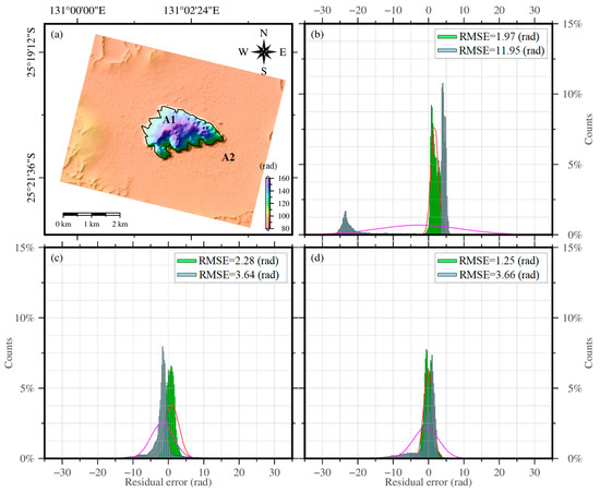
Figure 5.
Comparison of residual statistical results of the conventional InSAR (b), RSSI (c), and RID (d) methods. The light blue bar represents the residual distribution of A1 area in (a). The green bar represents the residual distribution of A2 area in (a). The red and purple curves represent the fitted probability distribution functions of the residual for A1 and A2, respectively.
4. Conclusions
This study proposed a range split-spectrum interferometry (RSSI)-assisted InSAR-derived DEM (RID) method to overcome phase-unwrapping errors. The performance of the RID method was verified using simulation and real data. The experiments show that the proposed method can significantly improve the influence of the phase-unwrapping errors of the conventional InSAR in generating DEM and compensate for the loss of resolution of the RSSI method. Additionally, this study concluded that the proposed method could provide an immediate DEM to overcome the difficulty of removing topographic errors in InSAR monitoring results of large gradient deformations using outdated DEM. Simultaneously, the proposed method provides the new idea of generating DEM from the new generation of dual-frequency SAR satellite images, such as NISAR and ALOS-4.
Author Contributions
Conceptualization, W.M., G.L. and X.W.; data curation, W.M. and X.W.; formal analysis, W.M., B.Z. and R.Z.; funding acquisition, G.L., X.W. and X.H.; investigation, W.X., S.W. and Y.F.; methodology, W.M., G.L. and X.W.; supervision, G.L. and X.W.; writing—original draft, W.M.; writing—review and editing, X.W., G.L., Y.X., X.H., B.Z. and S.P. All authors have read and agreed to the published version of the manuscript.
Funding
This work was funded in part by the National Natural Science Foundation of China (Grant numbers 42171355; 42071410; 41904002; 42104023); the Sichuan Science and Technology Program (Grant numbers 2019ZDZX0042; 2020YJ0322; 2020JDTD0003); the Jiangxi University of Science and Technology High-level Talent Research Startup Project (Grant numbers 205200100564; 205200100588); and the Cultivation Program for the Excellent Doctoral Dissertation of Southwest Jiaotong University (Grant number 2020YBPY12).
Data Availability Statement
Not applicable.
Acknowledgments
Some figures were generated by the Generic Mapping Tool version 6.0 (GMT 6.0) software [46].
Conflicts of Interest
The authors declare no conflict of interest.
References
- Shean, D.E.; Alexandrov, O.; Moratto, Z.M.; Smith, B.E.; Joughin, I.R.; Porter, C.; Morin, P. An automated, open-source pipeline for mass production of digital elevation models (DEMs) from very-high-resolution commercial stereo satellite imagery. ISPRS J. Photogramm. Remote Sens. 2016, 116, 101–117. [Google Scholar] [CrossRef] [Green Version]
- Wani, Z.M.; Nagai, M. An approach for the precise DEM generation in urban environments using multi-GNSS. Measurement 2021, 177, 109311. [Google Scholar] [CrossRef]
- Shan, J.; Aparajithan, S. Urban DEM generation from raw LiDAR data. Photogramm. Eng. Remote Sens. 2005, 71, 217–226. [Google Scholar] [CrossRef] [Green Version]
- Deilami, K.; Hashim, M. Very high resolution optical satellites for DEM generation: A review. Eur. J. Sci. Res. 2011, 49, 542–554. [Google Scholar]
- Rosen, P.A.; Hensley, S.; Joughin, I.R.; Li, F.K.; Madsen, S.N.; Rodriguez, E.; Goldstein, R.M. Synthetic aperture radar interferometry. Proc. IEEE 2000, 88, 333–382. [Google Scholar] [CrossRef]
- Del Soldato, M.; Confuorto, P.; Bianchini, S.; Sbarra, P.; Casagli, N. Review of works combining GNSS and InSAR in Europe. Remote Sens. 2021, 13, 1684. [Google Scholar] [CrossRef]
- Li, W.; Zhao, C.; Wang, B.; Zhang, Q. L1-Norm Sparse 2-D Phase Unwrapping Algorithm Based on Reliable Redundant Network. IEEE Geosci. Remote Sens. Lett. 2020, 19, 8004605. [Google Scholar] [CrossRef]
- Yu, H.; Lan, Y.; Yuan, Z.; Xu, J.; Lee, H. Phase unwrapping in InSAR: A review. IEEE Geosci. Remote Sens. Mag. 2019, 7, 40–58. [Google Scholar] [CrossRef]
- Zhang, W.; Zhu, W.; Tian, X.; Zhang, Q.; Zhao, C.; Niu, Y.; Wang, C. Improved DEM reconstruction method based on multibaseline InSAR. IEEE Geosci. Remote Sens. Lett. 2021, 19, 1–5. [Google Scholar] [CrossRef]
- Yuan, Z.; Deng, Y.; Li, F.; Wang, R.; Liu, G.; Han, X. Multichannel InSAR DEM reconstruction through improved closed-form robust Chinese remainder theorem. IEEE Geosci. Remote Sens. Lett. 2013, 10, 1314–1318. [Google Scholar] [CrossRef]
- Ferraiuolo, G.; Meglio, F.; Pascazio, V.; Schirinzi, G. DEM reconstruction accuracy in multichannel SAR interferometry. IEEE Trans. Geosci. Remote Sens. 2008, 47, 191–201. [Google Scholar] [CrossRef]
- Itoh, K. Analysis of the phase unwrapping algorithm. Appl. Opt. 1982, 21, 2470. [Google Scholar] [CrossRef] [PubMed]
- Yu, H.; Lan, Y. Robust two-dimensional phase unwrapping for multibaseline SAR interferograms: A two-stage programming approach. IEEE Trans. Geosci. Remote Sens. 2016, 54, 5217–5225. [Google Scholar] [CrossRef]
- Goldstein, R.M.; Zebker, H.A.; Werner, C.L. Satellite radar interferometry: Two-dimensional phase unwrapping. Radio Sci. 1988, 23, 713–720. [Google Scholar] [CrossRef] [Green Version]
- Costantini, M. A novel phase unwrapping method based on network programming. IEEE Trans. Geosci. Remote Sens. 1998, 36, 813–821. [Google Scholar] [CrossRef]
- Xu, J.; An, D.; Huang, X.; Yi, P. An efficient minimum-discontinuity phase-unwrapping method. IEEE Geosci. Remote Sens. Lett. 2016, 13, 666–670. [Google Scholar] [CrossRef]
- Flynn, T.J. Two-dimensional phase unwrapping with minimum weighted discontinuity. J. Opt. Soc. Am. A 1997, 14, 2692–2701. [Google Scholar] [CrossRef]
- Bioucas-Dias, J.M.; Valadao, G. Phase unwrapping via graph cuts. IEEE Trans. Image Process. 2007, 16, 698–709. [Google Scholar] [CrossRef]
- Chen, C.W.; Zebker, H.A. Two-dimensional phase unwrapping with use of statistical models for cost functions in nonlinear optimization. J. Opt. Soc. Am. A 2001, 18, 338–351. [Google Scholar] [CrossRef] [Green Version]
- Yu, H.; Xing, M.; Yuan, Z. Baseline Design for Multibaseline InSAR System: A Review. IEEE J. Miniat. Air Space Syst. 2020, 2, 17–24. [Google Scholar] [CrossRef]
- Yu, H.; Li, Z.; Bao, Z. A cluster-analysis-based efficient multibaseline phase-unwrapping algorithm. IEEE Trans. Geosci. Remote Sens. 2010, 49, 478–487. [Google Scholar] [CrossRef]
- Liu, H.; Xing, M.; Bao, Z. A cluster-analysis-based noise-robust phase-unwrapping algorithm for multibaseline interferograms. IEEE Trans. Geosci. Remote Sens. 2014, 53, 494–504. [Google Scholar] [CrossRef]
- Jiang, Z.; Wang, J.; Song, Q.; Zhou, Z. A refined cluster-analysis-based multibaseline phase-unwrapping algorithm. IEEE Geosci. Remote Sens. Lett. 2017, 14, 1565–1569. [Google Scholar] [CrossRef]
- Yuan, Z.; Lu, Z.; Chen, L.; Xing, X. A closed-form robust cluster-analysis-based multibaseline InSAR phase unwrapping and filtering algorithm with optimal baseline combination analysis. IEEE Trans. Geosci. Remote Sens. 2020, 58, 4251–4262. [Google Scholar] [CrossRef]
- Gao, Y.; Tang, X.; Li, T.; Lu, J.; Li, S.; Chen, Q.; Zhang, X. A phase slicing 2-D phase unwrapping method using the L1-norm. IEEE Geosci. Remote Sens. Lett. 2020, 19, 1–5. [Google Scholar] [CrossRef]
- Dai, Y.; Ng, A.H.-M.; Wang, H.; Li, L.; Ge, L.; Tao, T. Modeling-assisted InSAR phase-unwrapping method for mapping mine subsidence. IEEE Geosci. Remote Sens. Lett. 2020, 18, 1059–1063. [Google Scholar] [CrossRef]
- Simonyan, K.; Zisserman, A. Very deep convolutional networks for large-scale image recognition. arXiv 2014, arXiv:1409.1556. [Google Scholar]
- LeCun, Y.; Bengio, Y.; Hinton, G. Deep learning. Nature 2015, 521, 436–444. [Google Scholar] [CrossRef] [PubMed]
- Girshick, R.; Donahue, J.; Darrell, T.; Malik, J. Rich feature hierarchies for accurate object detection and semantic segmentation. In Proceedings of the IEEE Conference On Computer Vision and Pattern Recognition, Columbus, OH, USA, 23–28 June 2014; pp. 580–587. [Google Scholar]
- Zhang, J.; Tian, X.; Shao, J.; Luo, H.; Liang, R. Phase unwrapping in optical metrology via denoised and convolutional segmentation networks. Opt. Express 2019, 27, 14903–14912. [Google Scholar] [CrossRef] [Green Version]
- Spoorthi, G.; Gorthi, S.; Gorthi, R.K.S.S. PhaseNet: A deep convolutional neural network for two-dimensional phase unwrapping. IEEE Signal Process. Lett. 2018, 26, 54–58. [Google Scholar] [CrossRef]
- Zhang, T.; Jiang, S.; Zhao, Z.; Dixit, K.; Zhou, X.; Hou, J.; Zhang, Y.; Yan, C. Rapid and robust two-dimensional phase unwrapping via deep learning. Opt. Express 2019, 27, 23173–23185. [Google Scholar] [CrossRef] [PubMed]
- Spoorthi, G.; Gorthi, R.K.S.S.; Gorthi, S. PhaseNet 2.0: Phase unwrapping of noisy data based on deep learning approach. IEEE Trans. Image Process. 2020, 29, 4862–4872. [Google Scholar] [CrossRef]
- Wang, K.; Li, Y.; Kemao, Q.; Di, J.; Zhao, J. One-step robust deep learning phase unwrapping. Opt. Express 2019, 27, 15100–15115. [Google Scholar] [CrossRef]
- Wu, Z.; Wang, T.; Wang, Y.; Wang, R.; Ge, D. Deep Learning for the Detection and Phase Unwrapping of Mining-Induced Deformation in Large-Scale Interferograms. IEEE Trans. Geosci. Remote Sens. 2021, 60, 1–18. [Google Scholar] [CrossRef]
- Zhou, L.; Yu, H.; Lan, Y. Deep convolutional neural network-based robust phase gradient estimation for two-dimensional phase unwrapping using SAR interferograms. IEEE Trans. Geosci. Remote Sens. 2020, 58, 4653–4665. [Google Scholar] [CrossRef]
- Wu, Z.; Wang, T.; Wang, Y.; Wang, R.; Ge, D. Deep-learning-based phase discontinuity prediction for 2-D phase unwrapping of SAR interferograms. IEEE Trans. Geosci. Remote Sens. 2022, 60, 5216516. [Google Scholar] [CrossRef]
- Zhou, L.; Yu, H.; Lan, Y.; Gong, S.; Xing, M. CANet: An unsupervised deep convolutional neural network for efficient cluster-analysis-based multibaseline InSAR phase unwrapping. IEEE Trans. Geosci. Remote Sens. 2022, 60, 5212315. [Google Scholar] [CrossRef]
- Bamler, R.; Eineder, M. Accuracy of differential shift estimation by correlation and split-bandwidth interferometry for wideband and delta-k SAR systems. IEEE Geosci. Remote Sens. Lett. 2005, 2, 151–155. [Google Scholar] [CrossRef]
- Brcic, R.; Eineder, M.; Bamler, R. Interferometric absolute phase determination with TerraSAR-X wideband SAR data. In Proceedings of the 2009 IEEE Radar Conference, Pasadena, CA, USA, 4–8 May 2009; pp. 1–6. [Google Scholar]
- Brcic, R.; Eineder, M.; Bamler, R. Absolute phase estimation from TerraSAR-X acquisitions using wideband interferometry. In Proceedings of the 2018 IEEE Radar Conference, Rome, Italy, 26–30 May 2008. [Google Scholar]
- Yu, L.; Shan, X.-J.; Song, X.-G.; Qu, C.-Y. Deformation of the 2013 Pakistan MW7. 7 earthquake derived from sub-band InSAR. Chin. J. Geophys. 2016, 59, 1371–1382. [Google Scholar]
- Guth, P.L.; Geoffroy, T.M. LiDAR point cloud and ICESat-2 evaluation of 1 second global digital elevation models: Copernicus wins. Trans. GIS 2021, 25, 2245–2261. [Google Scholar] [CrossRef]
- Marešová, J.; Gdulová, K.; Pracná, P.; Moravec, D.; Gábor, L.; Prošek, J.; Barták, V.; Moudrý, V. Applicability of Data Acquisition Characteristics to the Identification of Local Artefacts in Global Digital Elevation Models: Comparison of the Copernicus and TanDEM-X DEMs. Remote Sens. 2021, 13, 3931. [Google Scholar] [CrossRef]
- Cenci, L.; Galli, M.; Palumbo, G.; Sapia, L.; Santella, C.; Albinet, C. Describing the Quality Assessment Workflow Designed for DEM Products Distributed Via the Copernicus Programme. Case Study: The Absolute Vertical Accuracy of the Copernicus DEM Dataset in Spain. In Proceedings of the 2021 IEEE International Geoscience and Remote Sensing Symposium IGARSS, Brussels, Belgium, 11–16 July 2021; pp. 6143–6146. [Google Scholar]
- Wessel, P.; Luis, J.; Uieda, L.; Scharroo, R.; Wobbe, F.; Smith, W.H.; Tian, D. The generic mapping tools version 6. Geochem. Geophys. Geosyst. 2019, 20, 5556–5564. [Google Scholar] [CrossRef] [Green Version]
Publisher’s Note: MDPI stays neutral with regard to jurisdictional claims in published maps and institutional affiliations. |
© 2022 by the authors. Licensee MDPI, Basel, Switzerland. This article is an open access article distributed under the terms and conditions of the Creative Commons Attribution (CC BY) license (https://creativecommons.org/licenses/by/4.0/).