High Spatiotemporal Rugged Land Surface Temperature Downscaling over Saihanba Forest Park, China

Abstract

Satellite-derived rugged land surface temperature (LST) is an important parameter indicating the status of the Earth’s surface energy budget and its seasonal/temporal dynamic change. However, existing LST products from rugged areas are more prone to error when supporting applications in mountainous areas and Earth surface processes that occur at high spatial and temporal resolutions. This research aimed to develop a method for generating rugged LST with a high temporal and spatial resolution by using an improved ensemble LST model combining three regressors, including a random forest, a ridge, and a support vector machine. Different combinations of high-resolution input parameters were also considered in this study. The input datasets included Moderate Resolution Imaging Spectroradiometer (MODIS) LST datasets (MxD11A1) for nighttime, temporal Sentinel-2 Multispectral Instrument (MSI) datasets, and digital elevation model (DEM) datasets. The 30 m rugged LST datasets derived were compared against an in situ LST dataset obtained at Saihanba Forest Park (SFP) sites and an ASTER-derived 90 m LST, respectively. The results with in situ measurements demonstrated significant LST details, with an R² higher than 0.95 and RMSE around 3.00 K for both Terra/MOD- and Aqua/MYD-based LST datasets, and with slightly better results being obtained from the Aqua/MYD-based LST than that from Terra/MOD. The inter-comparison results with ASTER LST showed that over 80% of the pixels of the difference image for the two datasets were within 2 K. In light of the complex topography and distinct atmospheric conditions, these comparison results are encouraging. The 30 m LST from the method proposed in this study also depicts the seasonality of rugged surfaces.

1. Introduction

Land surface temperature (LST), one of the Essential Climate Variables (ECV), is always identified as a critical, high-proof regional and global indicator for both climate and Earth energy balance [1,2]. Mountains account for about 24% of the Earth’s land surface [3,4], and are highly heterogeneous at both the temporal and spatial scales. Thus, high spatiotemporal (<100 m, about 1 day) LST products over mountainous areas from thermal satellite imagery are of great significance for local and regional research on budget balance and hydrothermal cycles [5].

However, there is currently a general lack of accurate rugged-area LST products with high spatial and high frequency coverage. The existing LST products from rugged areas are not sufficient to support applications involving mountainous areas or various Earth surface processes occurring at high spatial and temporal resolutions [6]. For example, the moderate surface temperature products (~1 km) [7,8,9,10,11] from the existing Moderate Resolution Imaging Spectroradiometer (MODIS) [12] have been widely distributed. Although their temporal resolution can reach about 1 day, and the accuracy can reach about 1 K on flat surfaces, the land surface heterogeneity caused by terrain effects is smoothed in the retrieval model, causing increased errors as a result of the heterogeneity of the land surface, as well as the influence of thermal radiation heterogeneity over rugged areas. Investigations have also shown that the errors caused by land surface heterogeneity can reach 9 K in mountain areas [13,14]; even the difference between shaded and sun-exposed surfaces can reach values greater than 30 K [15].

Currently, there are high-spatial-resolution sensors, such as Landsat-8 [16,17,18,19] and the Advanced Spaceborne Thermal Emission and Reflection Radiometer (ASTER) [20], that themselves directly use high-spatial-resolution satellite data for LST retrieval. However, the acquisition and parameterization of the characterization of rugged surfaces are still quite difficult in terms of LST and effective emissivity. For example, ASTER LST products only consider emissivity under homogeneous conditions [21,22], similar to the Landsat LST products [17]. The results obtained using LST retrieval methods over rugged surfaces are insufficient. Thus, the limitations of high-spatial-resolution thermal remote sensing data and the LST retrieval method have resulted in the loss of high-spatial-temporal LST products.

In order for LST to meet such spatial and temporal resolution requirements, downscaling is a potential method. Downscaling methods can be divided into two categories: the first are kernel-driven methods, in which the LST is downscaled using auxiliary data from multispectral sensors; the other are fusion-based methods, in which the information on temporal changes obtained from different sensors and neighborhood information are integrated to predict high-spatial-resolution LST [23]. The core of downscaling thermal images is inferential statistics; for example, the estimation of the emitted spectral characteristics of surface targets using finer spatial-resolution features from visible- and near-infrared (V-NIR) bands [24]. The feasibility of the downscaling methods depends on the availability of ancillary datasets. When ancillary datasets are limited, simple tools, such as linear and quadratic tools, are effective. Conversely, complex tools, such as artificial neural networks and machine-learning algorithms, can improve accuracy when ancillary datasets are abundant [24].

Although some researchers have reported higher resolution results based on current downscaling methods [25], reasonable accuracy can only be achieved at a spatial resolution of about 200–300 m [26] on flat surfaces. Furthermore, the performance of downscaling methods is more uncertain over rugged areas and might be affected by the lack of in situ measurements and the rugged topography [18]. Several studies have reported that machine-learning algorithms such as the random forest algorithm can be used to construct a reliable nonlinear relationship between LST and other important parameters, such as the normalized difference vegetation index (NDVI), digital elevation model (DEM) and albedo [27,28,29,30,31,32]. Downscaling with a single random forest regressor is always impacted by lower thermal contrasts in the image data, hindering the adequacy of training for the reproduction of temperature variations at a scale of ~250 m [32]. In order to improve the spatiotemporal resolution of LST in rugged areas, highly integrated machine-learning methods should be emphasized.

Thus, a method of LST downscaling is here proposed that integrates three machine-learning techniques to improve the spatiotemporal resolution of LST. The highly integrated nature of these three algorithms lessens the impact of the failure of a single one, making the method more robust. The selection of an ancillary dataset associated with the downscaling method was conducted specifically for a rugged area. The study area and the auxiliary data are illustrated in Section 2. The downscaling method is presented in Section 3. The validation and discussion of the method are presented in Section 4 and Section 5. Finally, the conclusions are summarized in Section 6.

2. Study Area and Data

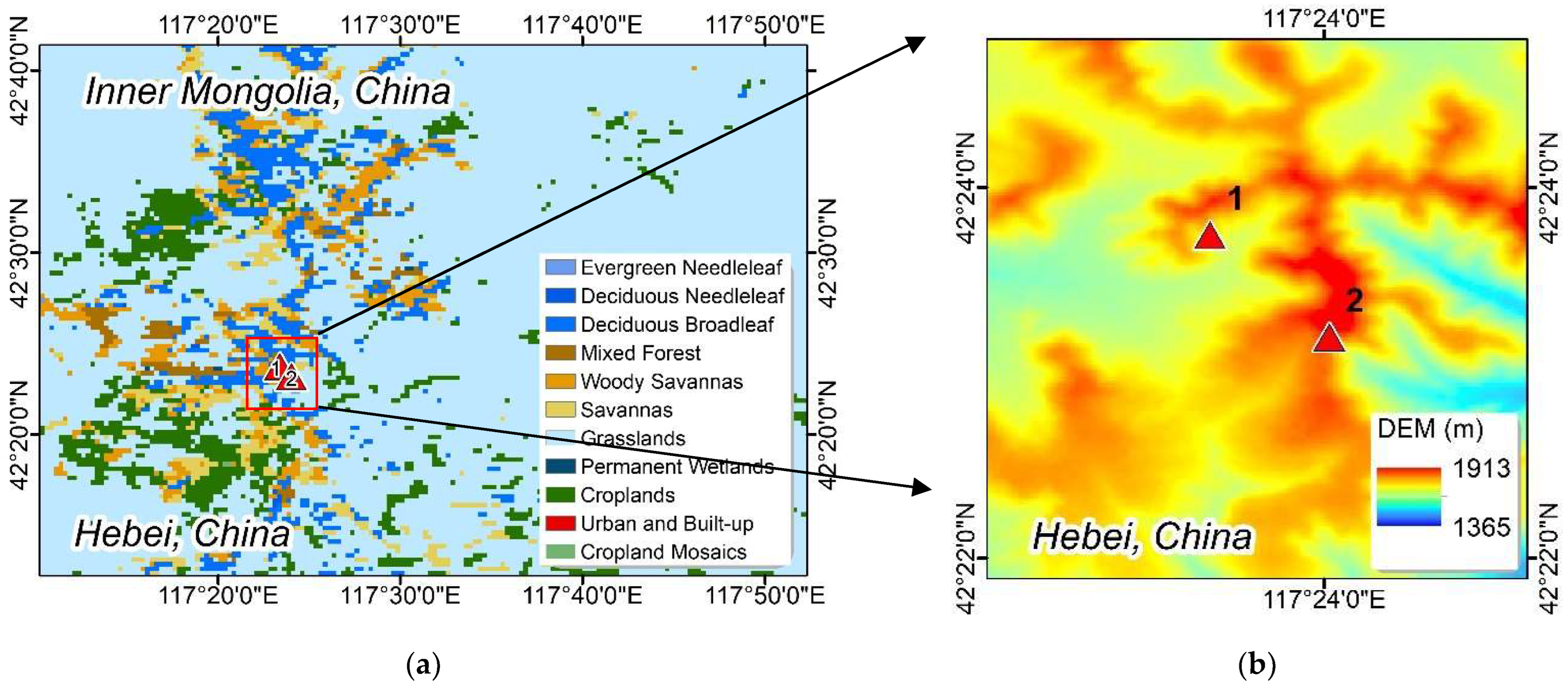
2.1. Study Area

Saihanba Forest Park (SFP) in northern China features a rugged topography, with a mean altitude of approximately 1700 m above sea level. It was set up in 1993 and covers a total area of 27,300 ha of semi-natural mixed deciduous–conifer forest. The carbon balance and water-use monitoring here are quite sensitive to surface temperature, which implies that the estimation of LST in this area is necessary to understand the effects of climate change [33,34]. A rugged study area located near Chengde City, Hebei Province, in the northeast of China was selected. It is characterized by rugged areas with an elevation not higher than 2000 m. The land cover of the study area and the SRTM 30 m DEM are presented in Figure 1. As shown in Figure 1, deciduous broadleaf and savannas are the predominant land types, and the land surface is rugged.

2.2. MODIS 1 km LST Datasets

Each MODIS sensor on board the EOS-Terra and EOS-Aqua satellites can provide daytime and nighttime passes and demonstrate a certain amount of quality control [35]. The daily 1 km LST datasets (MxD11A1), including MOD11A1 (MOD for short) and MYD11A1 (MYD for short), are often impeded by cloud coverage. Therefore, the available MODIS LST datasets have 1–4 day intervals, which means that the available images for MODIS 1 km LST from January to October might correspond to as little as 75 days or less following a year over the study area, counting both the MOD and the MYD. In addition, only nighttime LST (MOD11A1 and MYD11A1) datasets were used in this study in order to avoid the daytime uncertainty in both LST retrieval and validation in rugged areas. Detailed information about both MODIS LST products and the ancillaries utilized in this research is listed in

Table 1. MODIS datasets and ancillaries used in this research.

Product Name	Satellite	Datasets Name	Spatial Resolution	Temporal Resolution	View Time Coverage	Time Series	Number of Images Used
MOD11A1	Terra	LST	1 km	1–4 days	Night	2019.01–2019.10	112
MYD11A1	Aqua	LST	1 km	1–4 days	Night		99
MCD12Q1	Combined	Land cover (IGBP)	500 m	Yearly	2018	2018	1
-	Sentinel-2	NDVI	10 m	-	Multi-day	2019	17
-	Sentinel-2	WSA-VIS	10 m	-	Multi-day		17
SRTM1	SRTM	DEM	30 m	-	-	-	1

.

2.3. Sentinel-2 and SRTM Datasets

The Copernicus Sentinel-2 mission comprises twin satellites, Sentinel-2A and Sentinel-2B, in the same orbit and phased at 180 degrees (https://sentinel.esa.int/, accessed on 16 April 2021). This mission aims to provide high-spatial-resolution observations of land and coastal areas in the optical domain. It is able to fulfill the requirements of this research. Sentinel-2A was launched on 23 June 2015, while Sentinel-2B was launched on 7 March 2017. In this study, the Sentinel-2 datasets from January to October 2019 were used.

The revisit frequency of Sentinel-2 is 3–5 days, which is a high frequency for satellites with a spatial resolution of 10 m in the B2 (490 nm), B3 (560 nm), B4 (665 nm), and B8 (842 nm) bands. The Level-2A product from the Sentinel-2 multispectral instrument (MSI) can provide users with the BOA (bottom of the atmosphere) reflectance in Level-2A products, which are corrected for atmospheric, adjacency, and slope effects. It is derived on the basis of the Level-1C products.

The NDVI and the albedo for Sentinel-2, both 2A and 2B, as well as the VIS (Visible) broadband (0.30–0.70 μm) (albedo/VIS), are calculated on the basis of the Level-2A datasets in Google Earth Engine (GEE). The dataset characteristics are shown in Table 1.

The calculation methods for the NDVI and albedo/VIS are as follows:

$$NDVI=\frac{B8-B4}{B8+B4}$$

(1)

$$albedo/VIS=0.5673\times B2+0.1407\times B3+0.2359\times B4-0.0048$$

(2)

where B2, B3, B4, and B8 are the bands of the Sentinel-2 MSI. The coefficients from Equation (2) were obtained from [36]. Note that the spatial resolution of Sentinel-2 bands is 10 m. In this research, the 10 m original Sentinel-2 bands were first used to calculate NDVI and albedo/VIS; then, the products were resampled to 30 m using the nearest-neighbor method and reprojected to the Universal Transverse Mercator (UTM) projection. This projection was also used for the other datasets in this research.

The SRTM (Shuttle Radar Topography Mission) uses a radar dataset to successfully obtain an accurate global DEM, which is the leading input parameter in the production development of the LST datasets [37]. In this study, a 30 m (1 arc second) resolution SRTM1 dataset covering the study area was selected, which was downloaded from NASA Earthdata Search. The SRTM DEM can also be used to calculate the slope and aspect of each pixel.

2.4. In Situ Dataset

The accuracies of the traditional LST retrieval algorithms are usually validated in relatively flat places, whereas it is difficult to validate the rugged LST using in situ measurements, and less attention is paid to areas with complex topographies and distinct atmospheric conditions [6,33,38]. In this research, homogeneity was not a major consideration. Even if more heterogeneous surfaces yield lower spatial representativeness [39], we focused on the assessment of relative accuracy and the validation between in situ measurements and 30 m LST due to there being so many unstable parameters in rugged areas.

The relatively homogeneous grassland site measurements, taken at two sites in Saihanba Forest Park (SFP), were acquired between January and October 2019 [33,40,41]. The sites’ locations and detailed characteristics are presented in Figure 1 and

Table 2. Characteristics of the two SFP sites used in this study.

Site No.	Longitude (°E)	Latitude (°N)	Elevation (m)	Slope (°)	Aspect (°)	Land Surface Characteristics	Frequency	Period
1	117.3898	42.3957	1756.81	26	175	Mainly grass, three sides with trees but far away, sitting in the lower part of the mountain	Every minute	January–October 2019
2	117.4005	42.3865	1838.17	36	185	Mainly grass, with trees but far away, sitting in the top part of the mountain

. The ground sites represent different slopes and sit in different regions of the mountain. The slopes at site 1 and site 2 are 26 degrees and 36 degrees, respectively. The aspects of site 1 and site 2 are 175 degrees and 185 degrees, respectively. Further information about the sites can be found in [33] (Figure 1). Four-component radiation measurements from CNR4 net radiometers (Kipp & Zonen) were obtained every minute at both sites, and these were utilized to calculate the in situ LST corresponding to the simultaneous 30 m LST at nighttime. The CNR4 net radiometers were used to measure downward shortwave radiation (DSR) [33]. The in situ surface temperature was derived from the surface downwelling longwave (Rld, W/m²) and upwelling longwave radiation (Rlu, W/m²) along with the broadband emissivity [8,42,43], as shown in the following equation:

$$T={\left(\frac{Rlu-\left(1-\epsilon \right)Rld}{\epsilon ·\sigma }\right)}^{1/4}$$

(3)

where T (K) denotes the in situ measurements, which were used as the true values for the LST assessment. $\epsilon$ is the broadband surface emissivity, which was obtained from Landsat 8 Level 2 products sourced from the ASTER Global Emissivity Database (ASTER GED) [39]. $\sigma$ is the Stefan-Boltzmann constant.

2.5. ASTER-Derived 90 m LST Dataset

The Advanced Spaceborne Thermal Emission and Reflection Radiometer (ASTER) onboard EOS-Terra provides observations for three spectral regions with spatial resolutions of 15 m (visible and near-infrared, short wavelength infrared) and 90 m (thermal infrared) [20]. In this research, the ASTER-derived 90 m LST dataset, downloaded from NASA Earthdata Search (https://search.earthdata.nasa.gov/search, accessed on 1 March 2022), was used for the inter-comparison with the derived 30 m LST.

3. Methodology

V-NIR ancillary land surface parameters, such as NDVI and albedo, as well as the topographic effect, are important factors for deriving rugged LST time-series datasets with higher accuracy. To explore the relationship between LST and fine-resolution ancillary datasets in rugged areas, an improved ensemble LST model combining three regressors, including random forest, ridge, and support vector machine (SVM) regressors, was developed. The model was adapted from [29,30]. The LST model can be presented as the following equation:

$$LST=f(Elevation,Slope,Aspect,NDVI,Albedo)$$

(4)

where Elevation, Slope, and Aspect are taken from the DEM datasets, and NDVI and Albedo are calculated on the basis of the V-NIR satellite data from Sentinel-2. The core of this method is training the ensemble regression model and evaluating its performance. First, the datasets are randomly divided into training and test samples; 70% of the samples in this study were utilized to train the ensemble model, while the remaining 30% of the samples were used to evaluate the performance of the model. This 70/30 ratio is commonly used in machine learning. We used 70% as training samples and the rest were used as validation samples. This took into account not only the amount of training data, but also the number of test sets. Next, we created three regressors, namely random forest, ridge, and SVM regressors, and used random search and cross-validation to adjust their hyperparameters. The reason for the combination of these regressors applied here was the successful results from downscaling of LST using these three regressors in former studies [29,30,44]. After updating their hyperparameters, we used the ElasticNET linear regression model to stack the three regressors and fit the ensemble model to the training samples. Finally, we used the test samples to calculate the performance and return the ensemble model and calculated statistics.

Figure 2 shows the proposed method and the scheme from this research, which include the following major steps: (1) to ensure the number of samples for training the ensemble models and to avoid the MODIS cloud detection failure effect [45], satellite images with less than 40 percent of pixels missing (including cloud coverage) were chosen for the estimation of the nocturnal range data; otherwise, the images were excluded; (2) the ancillary data to be merged, including SRTM 30 m and Sentinel-2 NDVI/albedo 30 m, were prepared; (3) the regression parameters between the ancillary datasets and the MODIS 1 km LST nighttime products were constructed; (4) the 1 km coarse-scale LST datasets were downscaled to 30 m fine-resolution LST datasets using the regression parameters; and lastly, (5) the LST method was evaluated. Note that only nighttime MODIS LST datasets were considered in this study to simplify the environmental and planetary boundary layer (PBL) conditions in rugged areas during the daytime [8].

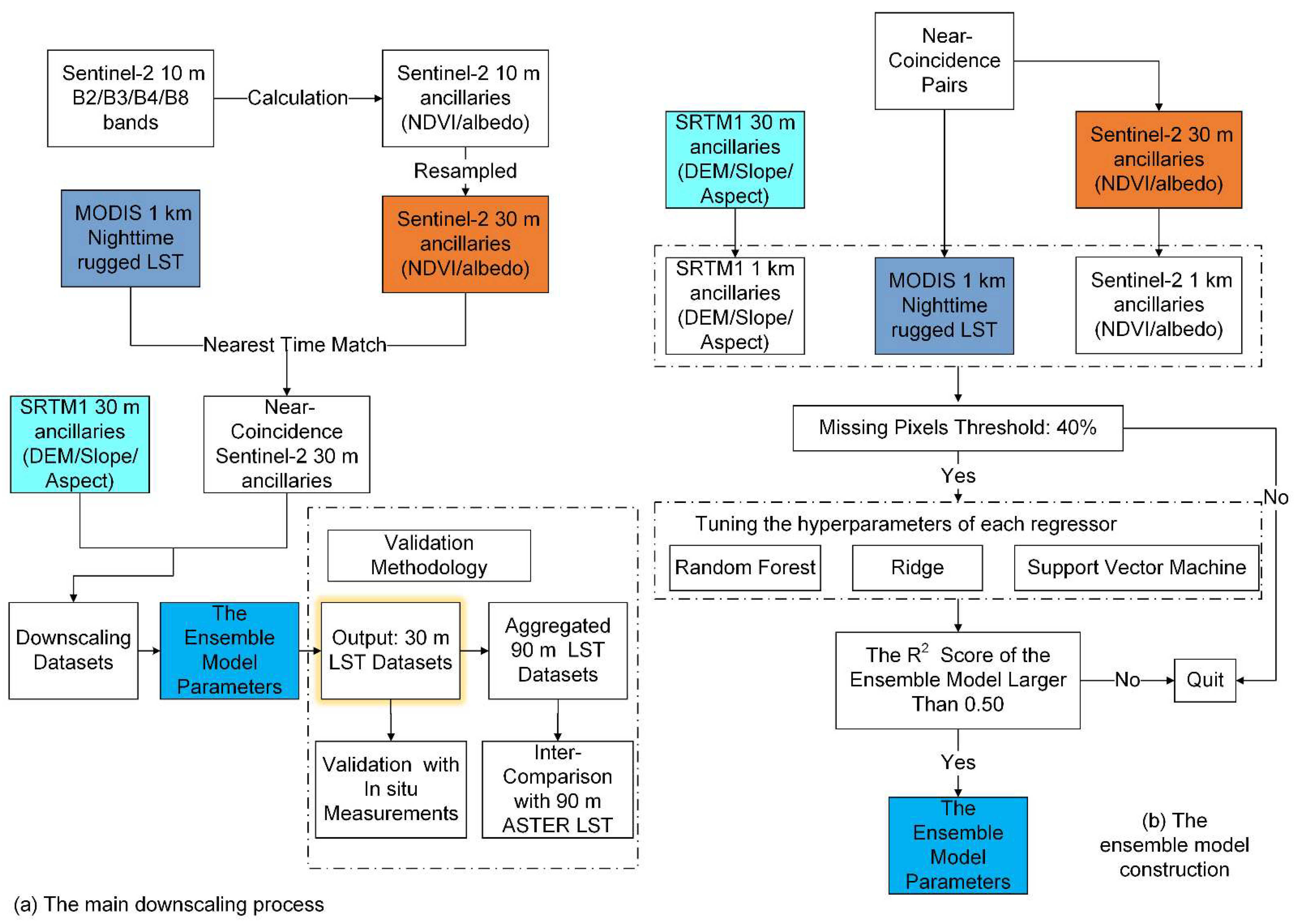
3.1. Methods of 30 m LST Retrieval from MODIS 1 km LST Time Series in Rugged Areas

To obtain finer resolution LST time-series datasets, basic MODIS 1 km LST datasets were the priority requirement. Ancillary datasets, including Sentinel-2 30 m NDVI, 30 m albedo/VIS, and SRTM1 30 m DEM, were utilized for the derivation of LST 30 m, as shown in Table 1.

The primary dataset was co-registered and built for the regression models with ancillary datasets (https://gdal.org/python/ (accessed on 2 May 2020)) to perform the resampling of the raster data and the scikit-learn library (https://scikit-learn.org/stable/ (accessed on 2 May 2020)) to build the regression parameters.

The ancillary datasets were selected by means of the physical principle used in the LST derivation. The physical principle used here was to choose the best combination of information from V-NIR bands to obtain the best understanding of the surface terrain. Recently, Yan [33] concluded that high-spatial-resolution DEM data and pre-defined spectral parameters are essential ancillaries for the radiative transfer model. Some researchers have shown that the correlation between NDVI and LST weakens during the night over North America [46], whereas other researchers have described 15 different indices over urban areas. The ancillary datasets used in the downscaling are different over local particularities of the land surface [30]. In this study, besides the detailed terrain description obtained from the DEM, the VIS albedo (0.30–0.70 μm) and NDVI were also selected, since they depict the spectral characteristics of rugged surfaces separately and can easily be obtained on the basis of sensor observations. The selection of the ancillaries was confirmed by the analysis presented in Section 4.1.

3.2. Assessment Methods for LST over the Study Area with In Situ Measurements

The spatial and temporal accuracy of the 30 m terrain LST was first assessed by means of in situ LST measurements. The matching in situ LST measurements both collocated in space and concurrent in time with the 30 m LST datasets were picked. The evaluation using the nighttime 30 m LST and ground measurements was performed for the period from January to October 2019. Two statistical criteria, including RMSE (root mean square error) and R² (coefficient of determination), were used for each ground site to assess the LST derivation results. The RMSE and R² equations are as follows:

$$RMSE=\sqrt{\frac{{\displaystyle \sum _{i=1}^n{(LS{T}_{30m}-LS{T}_{insitu})}^2}}{n}}$$

(5)

$$R^2={\left(\frac{{\displaystyle \sum (LS{T}_{30m}-\overline{LS{T}_{30m}})}(LS{T}_{insitu}-\overline{LS{T}_{insitu}})}{\sqrt{{\displaystyle \sum {(LS{T}_{30m}-\overline{LS{T}_{30m}})}^2{(LS{T}_{insitu}-\overline{LS{T}_{insitu}})}^2}}}\right)}^2$$

(6)

where $LS{T}_{30m}$ stands for the 30 m rugged LST, $LS{T}_{insitu}$ stands for the LST provided by the in situ measurements, $\overline{LS{T}_{30m}}$ stands for the average of $LS{T}_{30m}$, and $\overline{LS{T}_{insitu}}$ stands for the average of $LS{T}_{insitu}$.

3.3. Time-Series Analysis from the 30 m LST Dataset

The 30 m LST dataset was generated for the period between January and October 2019, which was an excellent period for the observation of temperature variations. To display both the high temporal and high spatial resolutions of the LST dataset, the time series from the in situ sites was used. For the spatial scale, two days from the LST dataset, one serving as a reference for spring and another as a reference for summer, were obtained. Then, the averaged spatial distribution of the LST from the study area over the course of 2019 was determined. For the temporal illustration, both the in situ LST and 30 m LST for the two validation sites were used for the period from January to October 2019. All of the cloud-free datasets from both the MOD- and MYD-derived 30 m LST were selected.

3.4. Inter-Comparison of 30 m Rugged LST and ASTER-Derived 90 m LST

Ideal validation sites are difficult to find, especially over non-flat and rugged terrain [47]. In this regard, in order to minimize the thermal heterogeneities caused by rugged terrain, an inter-comparison between the 30 m rugged LST derived in this research and the high-spatial-resolution ASTER-derived 90 m LST was also conducted to improve the evaluation processes.

First, the rugged 30 m LST was aggregated to a 90 m LST in order to match with the ASTER-derived 90 m LST. Then, a difference image for newly produced 90 m rugged LST and the ASTER LST was produced. Third, a histogram was produced for the difference image. Lastly, the inter-comparison results were analyzed.

4. Results

4.1. Ancillary Dataset Selection

Ancillary dataset selection should be the first step in the model design stage and is extremely important. It is strongly recommended that the selection of the ancillary dataset be performed carefully before any LST downscaling methods are applied in rugged areas.

Table 3. R² results from combinations of two parameters for one night obtained from MOD11A1 over SFP on 10 October 2019.

	WSA/VIS	NDVI	DEM
WSA/VIS	Fail	Fail	0.64
NDVI	-	Fail	0.60
DEM	-	-	Fail

demonstrates the R² results from two combinations for one night obtained from MOD11A1 over SFP on 10 October 2019.

As Table 3 indicates, using WSA/VIS, NDVI, or DEM alone all failed (threshold: R² less than 0.5) when using the proposed method. For combinations of two parameters, the R² of WSA/VIS and DEM reached 0.64, which was higher than those of the other two-parameter combinations. The combined use of more than three parameters was difficult to present in the same table; therefore, their description is presented in

Table 4. R² results from combinations of many parameters for one night obtained from MOD11A1 over SFP on 10 October 2019.

Combinations	R2
WSA/VIS + DEM + NDVI	0.70
WSA/VIS + DEM + ASPECT + SLOPE	0.65
WSA/VIS + NDVI + ASPECT + SLOPE	Fail
DEM + ASPECT + SLOPE	Fail
NDVI + DEM + ASPECT + SLOPE	0.61
WSA/VIS + NDVI + DEM + ASPECT + SLOPE	0.75

. The combination of five parameters received the highest score of 0.75. Although the use of greater numbers of parameters requires longer calculation times, using all five parameters together is still advised, as the ancillary datasets may provide better LST retrieval accuracy in the rugged areas of SFP than when using only two or three of them.

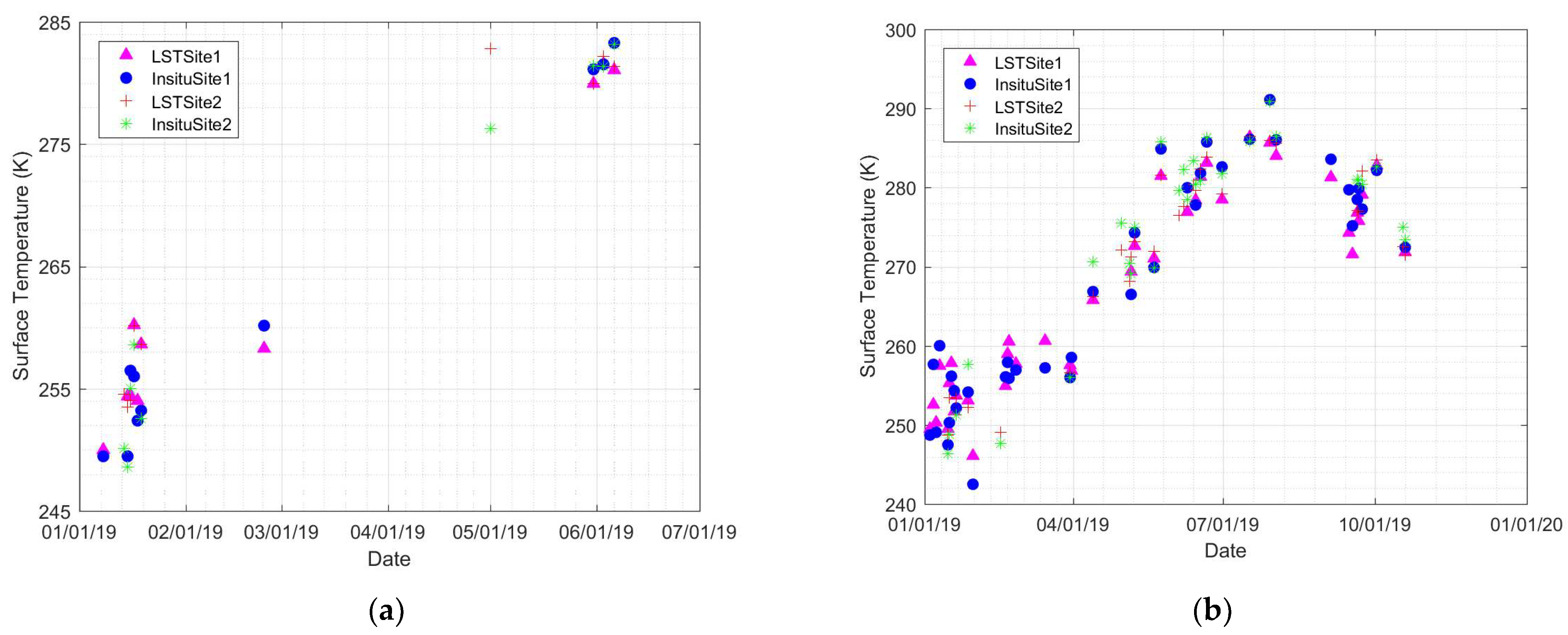
4.2. Comparison of Results for 30 m Rugged LST and In Situ Measurements

The derived 30 m rugged LST cloud-free products obtained using Sentinel-2 and DEM ancillaries were compared to in situ measurements from SFP.

Table 5. Assessment results for the ground sites vs. MODIS MOD and MYD nighttime 30 m LST products from January to October 2019.

Site No.	Terra/MOD-Based LST			Aqua/MYD-based LST
	RMSE (K)	R2	Samples	RMSE (K)	R2	Samples
1	2.95	0.96	10	2.75	0.97	39
2	3.84	0.95	9	2.92	0.96	30
ALL	3.40	0.96	19	2.83	0.97	69

demonstrates the statistical results obtained at site 1 and site 2, respectively, as well as the total results covering both ground sites.

The MOD- and MYD-derived 30 m LST are split into two parts. The Aqua/MYD passes over the study area late at night, at around 2:00 a.m., while the Terra/MOD passes over the study area at around 10:00 p.m. The total number of MODIS evaluation samples in Table 5 for the two ground sites obtained by the two sensors (Aqua and Terra) is 88. It is not normal for the number of samples obtained from Aqua/MYD (69) to be higher than that obtained from Terra/MOD (19). We believe that this might have been related to the different overpass times of the sensors in rugged areas. For the same reason, the MYD RMSE results were much better than those of MOD, with RMSEs less than 3.00 K at both site 1 and site 2. The R² values for all of the comparisons were greater than 0.95.

Figure 3 shows two scatter plots of 30 m LST estimated on the basis of the MOD and MYD datasets against the LST provided by in situ measurements. Although the slope at site 2 (36 degrees) is larger than that at site 1 (26 degrees), the assessment results for LST and in situ measurements were almost the same. The proposed 30 m rugged LST retrieval method showed encouraging performance for both slopes.

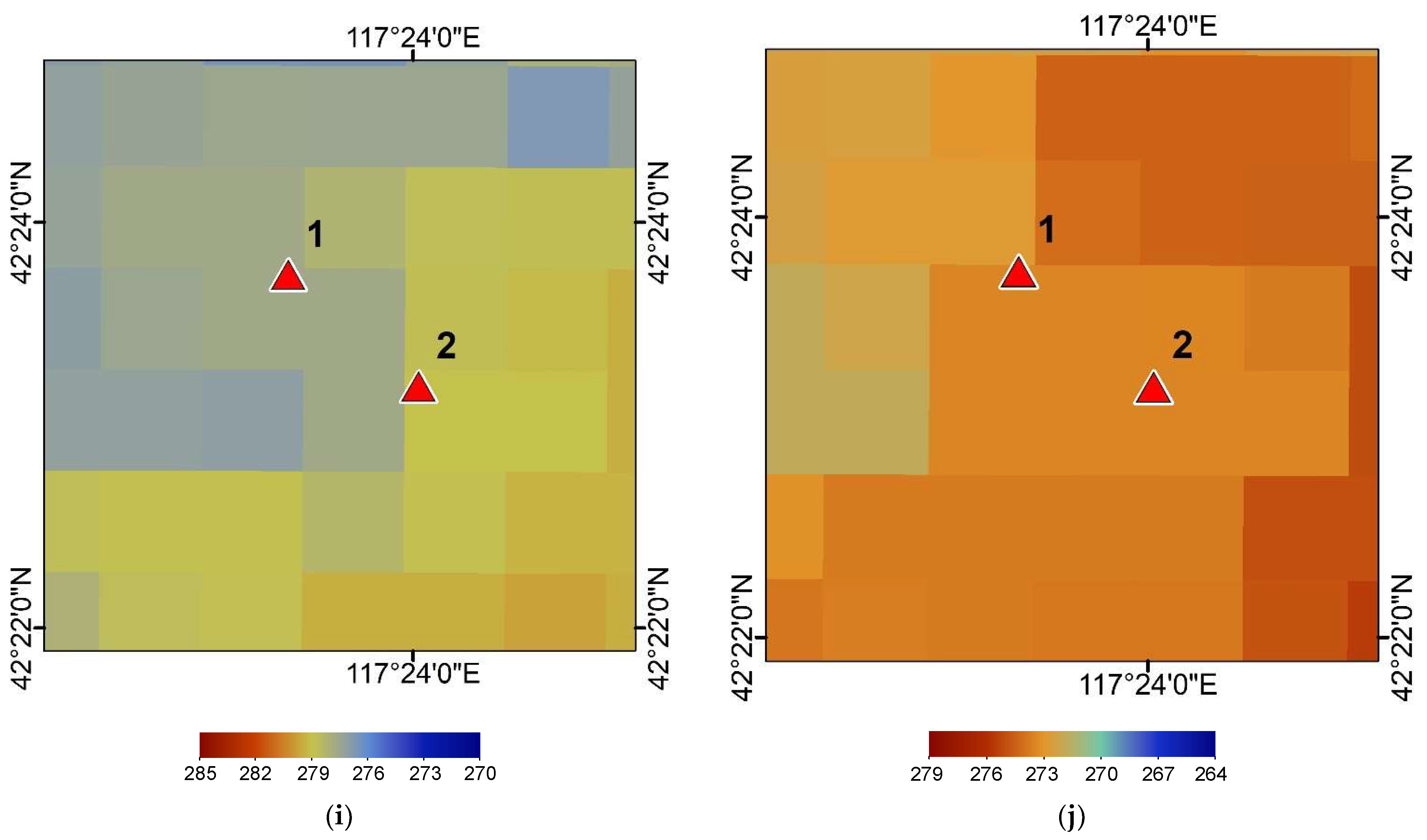
4.3. Temporal and Spatial Analysis from 30 m Rugged LST

The spatial distributions of the 30 m input datasets (DEM and NDVI), the 30 m LST nighttime average for 2019, the randomly selected 30 m LSTs, and the original 1 km LST are shown in Figure 4. Thanks to the ancillaries from DEM and Sentinel-2, these 30 m LSTs (Figure 4e,f) over SFP generally depicted the area well and provided texture with more detail than the 1 km MODIS LST (Figure 4i,j) alone. The spatial distribution from the 2:00 am (MYD) LST (Figure 4c,e) was much more uniform than that from the 10:00 pm (MOD) LST (Figure 4d,f) due to the late-night weather stability. This was also in agreement with the results from the previous part, suggesting that there are more cloud-free and available observations from Aqua/MYD than from Terra/MOD.

The LST datasets have a spatial resolution of 30 m, which is comparable to Sentinel-2 V-NIR products, but still have a higher temporal resolution than Sentinel-2. The selected LST results for 8 May, 9 May and 7 October 2019 clearly showed a temporal temperature change from summer to fall in rugged areas. The highest temperature recorded on 9 May was 288.64 K (Figure 4c), whereas the highest one recorded on 7 October was 270.13 K (Figure 4f). For the mean LST in 2019, the MOD- and MYD-derived LST datasets depict almost the same spatial distribution in Figure 4g,h.

A comparison of the cloud-free time series from 30 m LST and the in situ LST at in situ site 1 and site 2 for the period from January to October 2019 is presented in Figure 5. The surface temperature variations for the four seasons over the sites can be easily abstracted from the Aqua/MYD-derived 30 m LST (Figure 5b). Since the Terra/MOD-derived 30 m LST was not able to obtain a seasonal variation, only the Aqua/MYD-derived 30 m LST is considered in the following. The maximum LST at each site did not occur at the same time in the different datasets (with reference to the ground and satellite). The maximum in situ LSTs for both sites, which were also the maximum in both the ground and satellite datasets, occurred on 29 July 2019. The in situ LSTs for site 1 and site 2 were 291.12 K and 290.85 K, respectively. The maximum 30 m LST at each site occurred on 17 July 2019, a little earlier than the ground LST maximum date. The values for the maximum 30 m LSTs for site 1 and site 2 were 286.41 K and 286.48 K, respectively. The reason for the observed difference in the dates of the maximum LST between satellite and ground measurements was mainly due to the different scales of these datasets.

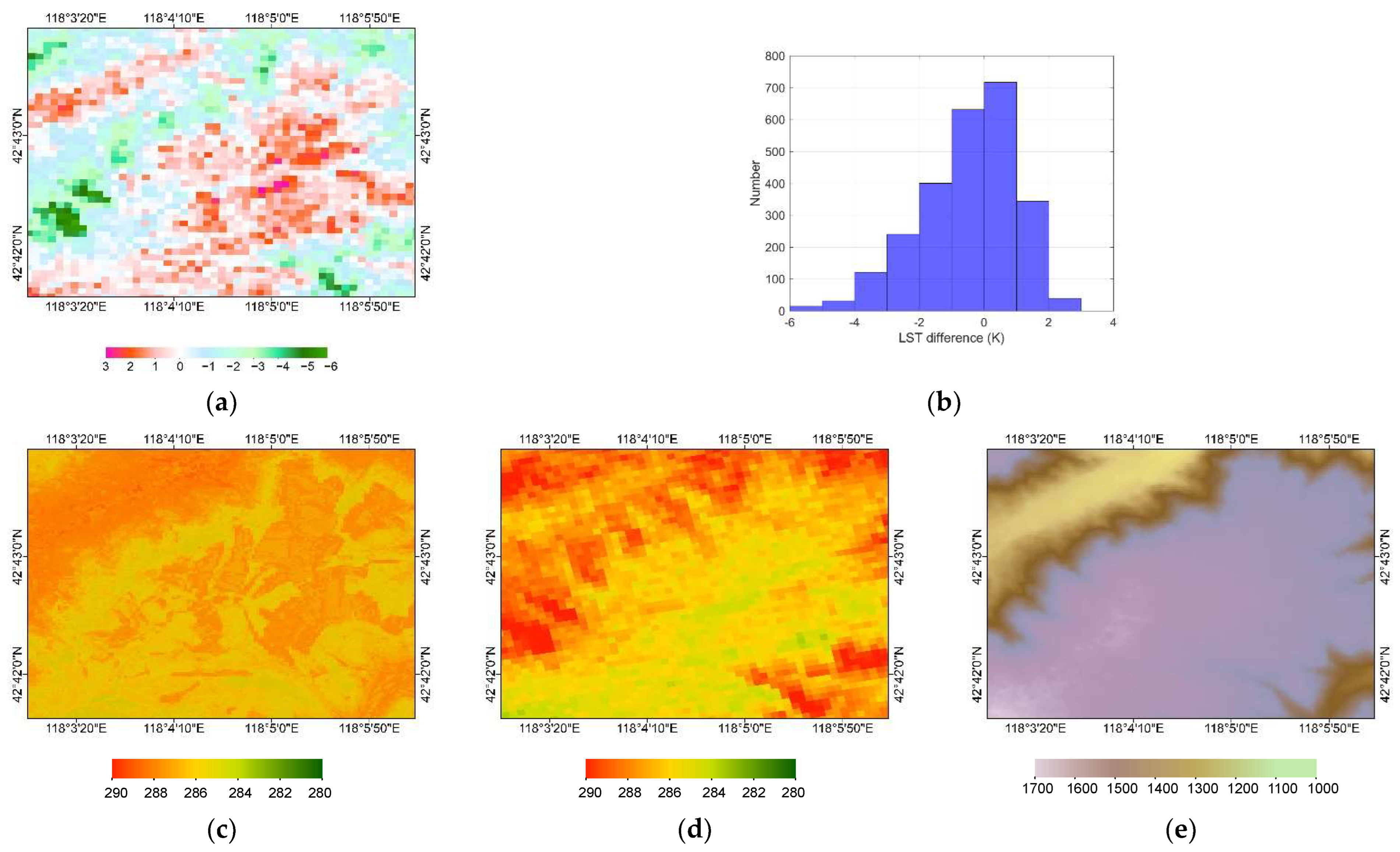
4.4. Inter-Comparison Results for 30 m Rugged LST and ASTER-Derived 90 m LST

In order to obtain a full understanding and to improve the evaluation of the retrieved 30 m rugged LST in the spatial scale, an inter-comparison of the results with the ASTER 90 m LST for regional purposes was also conducted, and the results are shown in Figure 6. Both images were acquired on 23 May 2019, and the 30 m LST was aggregated to 90 m in order to correspond to the spatial resolution of ASTER. As the ASTER swath width is narrower than that of MODIS, the ASTER footprint only passes through a corner of the MODIS image. In this study, no ASTER image was available that included the two validation sites. Since MODIS and ASTER are both on board the Terra satellite, their passing time is almost identical.

The difference image for the rugged 30 m LST and ASTER-derived 90 m LST and the corresponding difference histogram are shown in Figure 6a,b, respectively. The total number of pixels in Figure 6a is 2544. The difference pixels vary between a minimum of −6.07 K and a maximum of 2.99 K. A total of 53.03% of the pixels (1349/2544) are between −1 K and 1 K, while 82.31% of the pixels (2094/2544) are between −2 K and 2 K and 93.36% of pixels (2375/2544) are between −3 K and 3 K. When comparing Figure 6e, which shows the 30 m DEM image, the difference image distribution can be seen to be similar to the DEM spatial distribution to some extent. Clearly, the 30 m rugged LST (Figure 6c) depicts a more highly detailed LST distribution than the ASTER-derived LST (Figure 6d), with a difference of less than 2 K.

5. Discussion

5.1. Spatial Resolution and Selection Limitation in the Ancillary Dataset

The aim of this research was to develop a method for retrieving high-temporal- and high-spatial-resolution rugged LSTs that can be used for monitoring surface energy balance and fluxes. Much effort has been devoted to achieving this objective, and some encouraging results have been obtained. The spatial resolution of the major input parameters, such as the DEM, albedo, and NDVI, acts as a constraint on the output of the LST products. Thus, it is only possible to obtain 30 m LST due to the limited spatial resolution of the DEM input data. Conversely, if high-spatial-resolution input data were available, a high-spatial-resolution LST could also be obtained using the proposed method. Researchers can find other high-quality, high-spatial-resolution ancillary input datasets for LST retrieval using the proposed method. Note that this is not so difficult because the temporal resolution of the ancillaries is not mandatory. In this study, we only used a single DEM and 16-day NDVI/albedo (about 20 for each) for all calculations.

The results in Table 4 show that, when adding NDVI to WSA/VIS + DEM, the R² improved by 0.06. This means that the NDVI is extremely important for indicating the LST variations in rugged areas. It is difficult to explain the addition of ASPECT and SLOPE. When they were added to WSA/VIS + DEM, there was only an improvement in R² by 0.01. When they were added to NDVI + DEM, the R² also improved by 0.01. This means that the effect of adding ASPECT and SLOPE is negligible. However, when adding them to WSA/VIS + DEM + NDVI, the R² improved by 0.05. This might mean that the ASPECT and SLOPE work well with the other three ancillaries.

5.2. The Differences between Terra/MOD and Aqua/MYD

Another aspect is the different LSTs obtained from Terra/MOD and Aqua/MYD. These two original datasets are obtained using different sensors, although they are designed to have the same performance features as each other. The datasets were acquired at different times [42] and from different satellites. The land-surface heterogeneity and spatial characteristics were different due to the different acquisition times. Thus, the differences between these two sensors should be carefully considered in future LST analyses.

The different overpassing times of Terra/MOD (early night) and Aqua/MYD (mid-night) also produce different validation results. In the early night, thermal equilibrium in the rugged area was not achieved; thus, the ground measurements for the two sites were not able to represent the whole 30 m pixel. Conversely, the mid-night assessments performed better. This phenomenon also occurred during the daytime, when the thermal equilibrium is much more complex.

5.3. The Daytime 30 m Rugged LST and Its Validation

The third issue is that the daytime 30 m rugged LST datasets were also produced for the study area but not presented in this paper. As the energy turbulence and atmospheric conditions are much more complex over rugged areas in the daytime, it was difficult to obtain relatively homogeneous in situ measurements to validate the derived 30 m LST. Moreover, the surrounding rugged area provides non-negligible thermal radiation at the target pixels [6]. In addition, the uncertainty of daytime broadband emissivity, which is used for the in situ LST calculation, is twice that found at nighttime [19].

5.4. The Validation Issues with 30 m Rugged LST

This research did not focus on the rugged LST validation procedure, as the aim of this research was to discuss the possibility of 30 m rugged LST production from 1 km LST with ancillaries. Therefore, aspects related to the validation site and the LST comparison were not controlled as tightly as for the 1 km MODIS LST validation experiments [35,48,49]. In fact, the actual purpose of remote sensing products is to perform real-world spatial and temporal analyses in situations where strict control is usually not possible, especially in rugged areas. Therefore, comparisons between satellite-derived LSTs and LSTs obtained in situ are rather easier and more compatible than the strictly controlled validation of the LST algorithm over rugged areas.

In addition, the inter-comparison results were promising. Due to the small swath of ASTER and other environmental factors, only one matching inter-comparison pair was obtained during 2019. On the other hand, the scarcity of high-spatial-resolution images highlighted the importance of employing downscaling methods from moderate-resolution satellites over rugged areas.

5.5. Limitations of the Method

Although the proposed method achieved effective results over the rugged SFP with clear skies in northern China, it is still necessary to conduct further studies over rainy and rugged areas in southwest China, where the 1 km MODIS or other satellite datasets are not always available. In this study, we obtained almost 100 images for each MODIS sensor over the course of a year. It would not be possible to obtain this number in cloudy southwest China. In such places, the solution would be to use the reanalysis dataset and in situ measurements in order to obtain spatial and temporal LSTs [50]. Downscaling the 9 km reanalysis dataset over rugged areas remains a tremendous challenge. Still, the proposed method using a highly integrated machine-learning algorithm associated with DEM datasets may give scholars a method for downscaling LST over rugged and cloudy areas.

6. Conclusions

High-spatiotemporal-resolution LST is particularly important and is also a major controlling factor for monitoring regional surface energy balance and fluxes. In this study, we developed a feasible method for deriving 30 m rugged LST with both high spatial and temporal resolutions from MODIS LST products and Sentinel-2 V-NIR ancillaries. The proposed method was demonstrated to be able to provide high-spatial- and high temporal-resolution LST over rugged areas.

The relationships and the regression parameters between the LST and the fine-resolution V-NIR ancillary land surface parameters were firstly built using an improved ensemble LST model combining three regressors. Then, the 1 km MODIS LST nighttime products were downscaled to 30 m fine-resolution LST datasets on the basis of the regression parameters. This method is constrained by the spatial resolution of the V-NIR ancillaries; however, the temporal resolutions of the ancillaries are not mandatory.

The fine-resolution 30 m LST datasets for the year 2019 were compared against the SFP ground sites with different topographic conditions and different acquisition times. They were found to be in good agreement with the ground measurements, with an R² higher than 0.95 for different slopes (26 degrees and 36 degrees), different aspects (175 degrees and 185 degrees), and different MODIS LST datasets. The RMSEs from the Aqua/MYD-based LST (2.83 K) at 2 a.m. were slightly better than those of the Terra/MOD-based LST (3.40 K) at 10:00 p.m. This might have been related to the different satellite acquisition times and the four-component in situ measurement methods used over SFP. As a supplement to the in situ comparison, the inter-comparison with ASTER 90 m-derived LST showed promising results, with over 50% of the pixels from the difference being between -1 K and 1 K and over 80% of the pixels being between −2 K and 2 K. The proposed method using MODIS and Sentinel-2 datasets in order to obtain 30 m LST derivations depicts the rugged surfaces in greater detail, without losing any of the original accuracy of the 1 km MODIS LST datasets. In the future, a high-resolution digital surface model depicting the surface more accurately should be developed, and daytime validation should be performed in order to enhance LST retrieval and downscaling performances using much more detailed surface details.

References

1. Eleftheriou, D.; Kiachidis, K.; Kalmintzis, G.; Kalea, A.; Bantasis, C.; Koumadoraki, P.; Spathara, M.E.; Tsolaki, A.; Tzampazidou, M.I.; Gemitzi, A. Determination of annual and seasonal daytime and nighttime trends of MODIS LST over Greece-climate change implications. Sci. Total Environ. 2018, 616, 937–947. [Google Scholar] [PubMed]
2. GCOS. The Global Observing System for Climate: Implementation Needs; World Meteorological Organization: Geneva, Switzerland, 2016. [Google Scholar]
3. Meybeck, M.; Green, P.; Vörösmarty, C. A new typology for mountains and other relief classes. Mt. Res. Dev. 2001, 21, 34–45. [Google Scholar] [CrossRef] [Green Version]
4. Wen, J.; Liu, Q.; Xiao, Q.; Liu, Q.; You, D.; Hao, D.; Wu, S.; Lin, X. Characterizing land surface anisotropic reflectance over rugged terrain: A review of concepts and recent developments. Remote Sens. 2018, 10, 370. [Google Scholar]
5. Agam, N.; Kustas, W.P.; Anderson, M.C.; Li, F.; Colaizzi, P.D. Utility of thermal sharpening over Texas high plains irrigated agricultural fields. J. Geophys. Res. Atmos. 2007, 112. [Google Scholar] [CrossRef] [Green Version]
6. Wu, Y.; Wang, N.; Li, Z.; Chen, A.; Guo, Z.; Qie, Y. The effect of thermal radiation from surrounding terrain on glacier surface temperatures retrieved from remote sensing data: A case study from Qiyi Glacier, China. Remote Sens. Environ. 2019, 231, 111267. [Google Scholar] [CrossRef]
7. Ghent, D.; Corlett, G.; Göttsche, F.M.; Remedios, J. Global Land Surface Temperature From the Along-Track Scanning Radiometers. J. Geophys. Res. Atmos. 2017, 122, 12167–12193. [Google Scholar] [CrossRef] [Green Version]
8. Ouyang, X.; Chen, D.; Duan, S.-B.; Lei, Y.; Dou, Y.; Hu, G. Validation and Analysis of Long-Term AATSR Land Surface Temperature Product in the Heihe River Basin, China. Remote Sens. 2017, 9, 152. [Google Scholar] [CrossRef] [Green Version]
9. Pérez-Planells, L.; Niclòs, R.; Puchades, J.; Coll, C.; Göttsche, F.-M.; Valiente, J.A.; Valor, E.; Galve, J.M. Validation of Sentinel-3 SLSTR Land Surface Temperature Retrieved by the Operational Product and Comparison with Explicitly Emissivity-Dependent Algorithms. Remote Sens. 2021, 13, 2228. [Google Scholar] [CrossRef]
10. Yang, C.; Leonelli, F.E.; Marullo, S.; Artale, V.; Beggs, H.; Nardelli, B.B.; Chin, T.M.; De Toma, V.; Good, S.; Huang, B. Sea surface temperature intercomparison in the framework of the Copernicus Climate Change Service (C3S). J. Clim. 2021, 34, 5257–5283. [Google Scholar] [CrossRef]
11. Xu, W.; Wooster, M.J.; He, J.; Zhang, T. First study of Sentinel-3 SLSTR active fire detection and FRP retrieval: Night-time algorithm enhancements and global intercomparison to MODIS and VIIRS AF products. Remote Sens. Environ. 2020, 248, 111947. [Google Scholar]
12. Wan, Z. MODIS land-surface temperature algorithm theoretical basis document (LST ATBD). Inst. Comput. Earth Syst. Sci. St. Barbar. 1999. Available online: https://modis.gsfc.nasa.gov/data/atbd/atbd_mod11.pdf (accessed on 23 May 2022).
13. Yan, G.; Jiao, Z.-H.; Wang, T.; Mu, X. Modeling surface longwave radiation over high-relief terrain. Remote Sens. Environ. 2020, 237, 111556. [Google Scholar] [CrossRef]
14. Lipton, A.E.; Ward, J.M. Satellite-view biases in retrieved surface temperatures in mountain areas. Remote Sens. Environ. 1997, 60, 92–100. [Google Scholar] [CrossRef]
15. Raz-Yaseef, N.; Rotenberg, E.; Yakir, D. Effects of spatial variations in soil evaporation caused by tree shading on water flux partitioning in a semi-arid pine forest. Agric. For. Meteorol. 2010, 150, 454–462. [Google Scholar] [CrossRef]
16. Jiménez-Muñoz, J.C.; Sobrino, J.A.; Skoković, D.; Mattar, C.; Cristóbal, J. Land surface temperature retrieval methods from Landsat-8 thermal infrared sensor data. IEEE Geosci. Remote Sens. Lett. 2014, 11, 1840–1843. [Google Scholar] [CrossRef]
17. Malakar, N.K.; Hulley, G.C.; Hook, S.J.; Laraby, K.; Cook, M.; Schott, J.R. An operational land surface temperature product for Landsat thermal data: Methodology and validation. IEEE Trans. Geosci. Remote Sens. 2018, 56, 5717–5735. [Google Scholar] [CrossRef]
18. Cheng, J.; Meng, X.; Dong, S.; Liang, S. Generating the 30-m land surface temperature product over continental China and USA from landsat 5/7/8 data. Sci. Remote Sens. 2021, 4, 100032. [Google Scholar] [CrossRef]
19. Sekertekin, A.; Bonafoni, S. Sensitivity analysis and validation of daytime and nighttime land surface temperature retrievals from Landsat 8 using different algorithms and emissivity models. Remote Sens. 2020, 12, 2776. [Google Scholar] [CrossRef]
20. Abrams, M. The Advanced Spaceborne Thermal Emission and Reflection Radiometer (ASTER): Data products for the high spatial resolution imager on NASA’s Terra platform. Int. J. Remote Sens. 2000, 21, 847–859. [Google Scholar] [CrossRef]
21. Gillespie, A.R.; Abbott, E.A.; Gilson, L.; Hulley, G.; Jiménez-Muñoz, J.-C.; Sobrino, J.A. Residual errors in ASTER temperature and emissivity standard products AST08 and AST05. Remote Sens. Environ. 2011, 115, 3681–3694. [Google Scholar] [CrossRef]
22. Gillespie, A.R.; Matsunaga, T.; Rokugawa, S.; Hook, S.J. Temperature and emissivity separation from Advanced Spaceborne Thermal Emission and Reflection Radiometer (ASTER) images. In Proceedings of the SPIES International Symposium on Optical Science, Denver, CO, USA, 4 August 1996. [Google Scholar]
23. Xia, H.; Chen, Y.; Li, Y.; Quan, J. Combining kernel-driven and fusion-based methods to generate daily high-spatial-resolution land surface temperatures. Remote Sens. Environ. 2019, 224, 259–274. [Google Scholar] [CrossRef]
24. Zhan, W.F.; Chen, Y.H.; Zhou, J.; Wang, J.F.; Liu, W.Y.; Voogt, J.; Zhu, X.L.; Quan, J.L.; Li, J. Disaggregation of remotely sensed land surface temperature: Literature survey, taxonomy, issues, and caveats. Remote Sens. Environ. 2013, 131, 119–139. [Google Scholar] [CrossRef]
25. Sánchez, J.M.; Galve, J.M.; González-Piqueras, J.; López-Urrea, R.; Niclòs, R.; Calera, A. Monitoring 10-m LST from the Combination MODIS/Sentinel-2, Validation in a High Contrast Semi-Arid Agroecosystem. Remote Sens. 2020, 12, 1453. [Google Scholar] [CrossRef]
26. Pu, R.L. Assessing scaling effect in downscaling land surface temperature in a heterogenous urban environment. Int. J. Appl. Earth Obs. Geoinf. 2021, 96, 102256. [Google Scholar] [CrossRef]
27. Zhao, W.; Duan, S.-B. Reconstruction of daytime land surface temperatures under cloud-covered conditions using integrated MODIS/Terra land products and MSG geostationary satellite data. Remote Sens. Environ. 2020, 247, 111931. [Google Scholar] [CrossRef]
28. Zhou, J.; Liu, S.; Li, M.; Zhan, W.; Xu, Z.; Xu, T. Quantification of the scale effect in downscaling remotely sensed land surface temperature. Remote Sens. 2016, 8, 975. [Google Scholar] [CrossRef] [Green Version]
29. Sismanidis, P. Applying Computational Methods for Processing Thermal Satellite Images of Urban Areas. Ph.D. Thesis, School of Chemical Engineering, National Technical University of Athens, Athens, Greece, 2018. [Google Scholar]
30. Sismanidis, P.; Keramitsoglou, I.; Bechtel, B.; Kiranoudis, C.T. Improving the downscaling of diurnal land surface temperatures using the annual cycle parameters as disaggregation kernels. Remote Sens. 2017, 9, 23. [Google Scholar] [CrossRef] [Green Version]
31. Yang, G.; Pu, R.; Zhao, C.; Huang, W.; Wang, J. Estimation of subpixel land surface temperature using an endmember index based technique: A case examination on ASTER and MODIS temperature products over a heterogeneous area. Remote Sens. Environ. 2011, 115, 1202–1219. [Google Scholar] [CrossRef]
32. Hutengs, C.; Vohland, M. Downscaling land surface temperatures at regional scales with random forest regression. Remote Sens. Environ. 2016, 178, 127–141. [Google Scholar] [CrossRef]
33. Yan, G.; Chu, Q.; Tong, Y.; Mu, X.; Qi, J.; Zhou, Y.; Liu, Y.; Wang, T.; Xie, D.; Zhang, W. An Operational Method for Validating the Downward Shortwave Radiation Over Rugged Terrains. IEEE Trans. Geosci. Remote Sens. 2020, 59, 714–731. [Google Scholar] [CrossRef]
34. Li, L.; Chen, J.; Mu, X.; Li, W.; Yan, G.; Xie, D.; Zhang, W. Quantifying understory and overstory vegetation cover using UAV-based RGB imagery in forest plantation. Remote Sens. 2020, 12, 298. [Google Scholar] [CrossRef] [Green Version]
35. Wan, Z.; Zhang, Y.; Zhang, Q.; Li, Z.L. Quality assessment and validation of the MODIS global land surface temperature. Int. J. Remote Sens. 2004, 25, 261–274. [Google Scholar] [CrossRef]
36. Li, Z.; Erb, A.; Sun, Q.; Liu, Y.; Shuai, Y.; Wang, Z.; Boucher, P.; Schaaf, C. Preliminary assessment of 20-m surface albedo retrievals from sentinel-2A surface reflectance and MODIS/VIIRS surface anisotropy measures. Remote Sens. Environ. 2018, 217, 352–365. [Google Scholar] [CrossRef]
37. Werner, M. Shuttle Radar Topography Mission (SRTM) Mission Overview. Frequenz 2001, 55, 75–79. [Google Scholar] [CrossRef]
38. Coll, C.; Caselles, V.; Galve, J.M.; Valor, E.; Niclos, R.; Sanchez, J.M.; Rivas, R. Ground measurements for the validation of land surface temperatures derived from AATSR and MODIS data. Remote Sens. Environ. 2005, 97, 288–300. [Google Scholar] [CrossRef]
39. Hulley, G.C.; Hook, S.J.; Abbott, E.; Malakar, N.; Islam, T.; Abrams, M. The ASTER Global Emissivity Dataset (ASTER GED): Mapping Earth’s emissivity at 100 meter spatial scale. Geophys. Res. Lett. 2015, 42, 7966–7976. [Google Scholar] [CrossRef]
40. Yan, G.; Tong, Y.; Yan, K.; Mu, X.; Chu, Q.; Zhou, Y.; Liu, Y.; Qi, J.; Li, L.; Zeng, Y. Temporal extrapolation of daily downward shortwave radiation over cloud-free rugged terrains. Part 1: Analysis of topographic effects. IEEE Trans. Geosci. Remote Sens. 2018, 56, 6375–6394. [Google Scholar] [CrossRef]
41. Zhou, Y.; Yan, G.; Zhao, J.; Chu, Q.; Liu, Y.; Yan, K.; Tong, Y.; Mu, X.; Xie, D.; Zhang, W. Estimation of daily average downward shortwave radiation over Antarctica. Remote Sens. 2018, 10, 422. [Google Scholar] [CrossRef] [Green Version]
42. Cheng, J.; Liang, S.L.; Yao, Y.J.; Zhang, X.T. Estimating the Optimal Broadband Emissivity Spectral Range for Calculating Surface Longwave Net Radiation. IEEE Geosci. Remote Sens. Lett. 2013, 10, 401–405. [Google Scholar] [CrossRef]
43. Wang, K.; Liang, S. Evaluation of ASTER and MODIS land surface temperature and emissivity products using long-term surface longwave radiation observations at SURFRAD sites. Remote Sens. Environ. 2009, 113, 1556–1565. [Google Scholar] [CrossRef]
44. Keramitsoglou, I.; Kiranoudis, C.T.; Weng, Q. Downscaling geostationary land surface temperature imagery for urban analysis. IEEE Geosci. Remote Sens. Lett. 2013, 10, 1253–1257. [Google Scholar] [CrossRef]
45. Kokalj, Ž.; Somrak, M. Why not a single image? Combining visualizations to facilitate fieldwork and on-screen mapping. Remote Sens. 2019, 11, 747. [Google Scholar] [CrossRef] [Green Version]
46. Sun, D.; Kafatos, M. Note on the NDVI-LST relationship and the use of temperature-related drought indices over North America. Geophys. Res. Lett. 2007, 34. [Google Scholar] [CrossRef] [Green Version]
47. Guillevic, P.; Göttsche, F.; Nickeson, J.; Hulley, G.; Ghent, D.; Yu, Y.; Trigo, I.; Hook, S.; Sobrino, J.; Remedios, J. Land surface temperature product validation best practice protocol. Version 1.1. Best Pract. Satell.—Deriv. Land Prod. Valid. 2018, 60. [Google Scholar] [CrossRef]
48. Wan, Z.; Zhang, Y.; Zhang, Q.; Li, Z.-L. Validation of the land-surface temperature products retrieved from Terra Moderate Resolution Imaging Spectroradiometer data. Remote Sens. Environ. 2002, 83, 163–180. [Google Scholar] [CrossRef]
49. Bosilovich, M.G. A comparison of MODIS land surface temperature with in situ observations. Geophys. Res. Lett. 2006, 33. [Google Scholar] [CrossRef]
50. Jia, A.; Ma, H.; Liang, S.; Wang, D. Cloudy-sky land surface temperature from VIIRS and MODIS satellite data using a surface energy balance-based method. Remote Sens. Environ. 2021, 263, 112566. [Google Scholar] [CrossRef]
Figure 1. Land cover of the study area in SFP (a) and the SRTM 30 m DEM of the validation stations (b). The land-cover map was obtained from the MODIS land-cover product MCD12Q1 in 2018, in which the International Geosphere–Biosphere Program (IGBP) global vegetation classification was chosen. The two in situ sites in SFP are indicated by the red triangles.
Remotesensing 14 02617 g001
Figure 2. Flowchart of the proposed method and the scheme of this research. (a) The main downscaling process; (b) construction of the ensemble model.
Remotesensing 14 02617 g002
Figure 3. The scatter plots for nighttime temperature at the SFP sites using 30 m LST and in situ measurements from January to October 2019: (a) Terra/MOD (around 10:00 p.m.); (b) Aqua/MYD (around 2:00 a.m.).
Remotesensing 14 02617 g003
Figure 4. Spatial distribution of the (a) DEM, (b) NDVI, (c) nighttime LST on 9 May from MOD, (d) nighttime 30 m LST on 8 May from MYD, (e) nighttime 30 m LST on 7 October from MOD, (f) nighttime 30 m LST on 7 October from MYD, (g) 30 m LST nighttime average for 2019 from MOD, (h) 30 m LST nighttime average for 2019 from MYD, (i) nighttime 1 km LST on 9 May from MOD, (j) nighttime 1 km LST on 8 May from MYD. Note that the LST images are from different acquisition days and times, and thus the legend cannot use the same range.
Remotesensing 14 02617 g004aRemotesensing 14 02617 g004bRemotesensing 14 02617 g004c
Figure 5. Cloud-free time-series comparison between 30 m LST and in situ LST at site 1 and site 2 from January to October 2019: (a) MOD; (b) MYD.
Remotesensing 14 02617 g005
Figure 6. Inter-comparison images for the rugged 30 m LST (aggregated to 90 m) and ASTER-derived 90 m LST. (a) The difference between the rugged 30 m LST (aggregated to 90 m) and ASTER-derived 90 m LST; (b) the histogram corresponding to the difference image; (c) 30 m rugged LST; (d) ASTER-derived 90 m LST; (e) 30 m DEM.
Remotesensing 14 02617 g006