Shadow Removal from UAV Images Based on Color and Texture Equalization Compensation of Local Homogeneous Regions

Abstract

Due to imaging and lighting directions, shadows are inevitably formed in unmanned aerial vehicle (UAV) images. This causes shadowed regions with missed and occluded information, such as color and texture details. Shadow detection and compensation from remote sensing images is essential for recovering the missed information contained in these images. Current methods are mainly aimed at processing shadows with simple scenes. For UAV remote sensing images with a complex background and multiple shadows, problems inevitably occur, such as color distortion or texture information loss in the shadow compensation result. In this paper, we propose a novel shadow removal algorithm from UAV remote sensing images based on color and texture equalization compensation of local homogeneous regions. Firstly, the UAV imagery is split into blocks by selecting the size of the sliding window. The shadow was enhanced by a new shadow detection index (SDI) and threshold segmentation was applied to obtain the shadow mask. Then, the homogeneous regions are extracted with LiDAR intensity and elevation information. Finally, the information of the non-shadow objects of the homogeneous regions is used to restore the missed information in the shadow objects of the regions. The results revealed that the average overall accuracy of shadow detection is 98.23% and the average F1 score is 95.84%. The average color difference is 1.891, the average shadow standard deviation index is 15.419, and the average gradient similarity is 0.726. The results have shown that the proposed method performs well in both subjective and objective evaluations.

1. Introduction

Shadow in remote sensing images is a phenomenon of image degradation that results in the absence of image features or low definition due to light being completely or partially blocked by objects [1,2]. With the advantages of high resolution, low acquisition cost, and fast acquisition speed, unmanned aerial vehicle (UAV) images have become popular in practice for collecting data and mapping [3]. However, due to the compound effect of solar illumination, ground reflection, and atmospheric disturbance, UAV remote sensing images widely suffer from the problem of low recognition of color features and texture features in shadow regions, which seriously reduces the quality of UAV remote sensing images, and then has serious impact on subsequent image processing tasks such as image interpretation, image matching, feature extraction, land cover classification, and digital photogrammetry [4,5,6,7]. Although there are ways to automatically balance in the case of UAV cameras, for example, the DJI GO app has automatic light balance in order to avoid darkness or high exposure, it can only optimize for uneven lighting, not eliminate shadows. How to effectively extract shadows and compensate the color and texture information in the shadowed regions is especially important. However, the current shadow detection and compensation methods [8,9,10,11] are still a challenging task in dealing with the shadows of UAV images with complex surface features and a wide variety of objects.

In order to effectively reduce the effects of shadows on remote sensing images, many researchers have been devoted to developing techniques for shadow detection and compensation from remote sensing images. Accurate shadow detection is an important prerequisite for shadow compensation. Shadow detection methods can be divided into two main categories: model-based and feature-based methods [12,13,14,15,16,17,18]. The model-based methods require a lot of prior information. For example, the sensor’s position, digital elevation model (DEM), and solar azimuth. Such information is difficult to obtain in the research process, which greatly limits the application scope of this method [19,20,21,22]. At present, feature-based methods are mainly used to study the color features of the image, and shadow extraction is carried out by using the color characteristics of the pixel gray scale of the shadow area in RGB, HSV, YCbCr, and other color spaces [23,24]. Tasi et al. [25] calculate the global threshold of ratio image by the ratio of hue-equivalent components to intensity-equivalent components. This threshold is applied to segment the image to obtain the shadow regions. However, the shadow detection effect is weakened when the influence of objects is complex. Based on the work of Tsai, Zhou et al. [26] defined the shadow index (SI) based on the YCbCr space to extract shadow. However, the SI is susceptible to high-reflectance objects such as white vehicles in the shadow region, and requires NIR bands to improve SI. The shadow regions have the maximum value of the saturation component and the minimum value of the value component in the HSV color space. Based on this particular property of shadows, a normalized saturation-value difference index (NSVDI) is constructed by Ma et al. [27] to identify shadows. However, due to the similarity of spectrum, some dark objects still cannot be distinguished from shadows. In conclusion, existing shadow detection methods have limited application conditions, and the accurate shadow detection of UAV RGB remote sensing images needs further research.

Shadow compensation is a restoring process to improve image quality and enhance image visual effects. Although information in shadowed regions is obscured, some effective information is still contained in shadow images. This provides the possibility of restoring surface feature information of the shadowed regions [28]. However, shadow compensation cannot fully restore the occluded information, as shadows are formed by a complex composite function of solar illumination, ground reflection, and atmospheric disturbances. Hence, many shadow compensation methods are dedicated to restoring surface feature information in the shadow area to some extent, rather than fully restoring it [29,30]. The key of shadow compensation is to restore the maximum amount of color and texture detail information in the shadow regions without disturbing the feature information in the non-shadow regions of the image.

The existing shadow compensation strategies [31,32,33,34,35,36,37] can be broadly classified into two types, namely, local and global strategies. The global strategy takes the whole image into consideration directly, and compensates the information of the shadow regions by global optimization [38]. It can remove the shadows in whole directly, but it is not good at restoring color and texture details in images, especially for high-resolution UAV remote sensing images with a complex background and multiple shadows. Comparatively, the local strategy restores overs information of a shadow pixel or region based on the information of adjacent non-shadow features. For example, Zhou et al. [26] used the mean-shift algorithm to segment the image and compensated the shadow illumination by matching adjacent objects. Based on Markov random field theory, Song et al. [39] constructed a matching relation between shadow region and non-shadow region to improve the accuracy of shadow compensation. Silva et al. [40] proposed an algorithm based on the spatial distribution of adjacent pixels, which effectively improves the sharpness of the shadow region of the original image. Overall, the global strategy can produce better shadow compensation results, but still has some shortcomings in dealing with the shadows of UAV images with complex surface features and a wide variety of objects. For example, a local color transfer algorithm is proposed by Gilberto et al. [41] which can accurately correct the color without losing texture information, but the restored image has obvious shadow boundaries. Therefore, how to accurately compensate for shadows remains to be studied in more depth.

Recently, some researchers have taken advantage of the LiDAR to solve the segmentation and detection problems in image processing. For example, Awad [42] demonstrated that the combination of LiDAR data with optical images helps improve the accuracy of image segmentation by reducing over-segmentation and confusion between similar materials. Han et al. [43] proposed a road detection method based on the fusion of LiDAR and image data, and the results proved that the fused features can improve the performance of road detection. Based on the above inspiration, we propose a novel shadow removal algorithm for UAV remote sensing images, which is based on color and texture equalization compensation of locally homogeneous regions to solve the problem of obvious heterogeneity between shadow and non-shadow regions compensated by existing methods.

The main contributions and advantages of the proposed approach are as follows: (1) A novel algorithm is proposed to remove shadows from UAV remote sensing images based on color and texture equalization compensation of local homogeneous regions, which can not only effectively recover color and texture details of shadowed objects, but also well preserve the surface feature information in non-shadow regions; (2) The new shadow detection index is defined based on the R, G, and B bands of a UAV image, which can effectively enhance the shadow; (3) A homogeneous region segmentation method is proposed based on LiDAR data, using the LiDAR intensity and elevation range of typical objects as the basis for homogeneous regions extraction to achieve accurate extraction of homogeneous regions.

The rest of paper is organized as below. Section 2 explains in detail the methodology of the proposed method. Section 3 presents the experimental design and the experimental results. Discussion and conclusions are shown in Section 4 and Section 5, respectively.

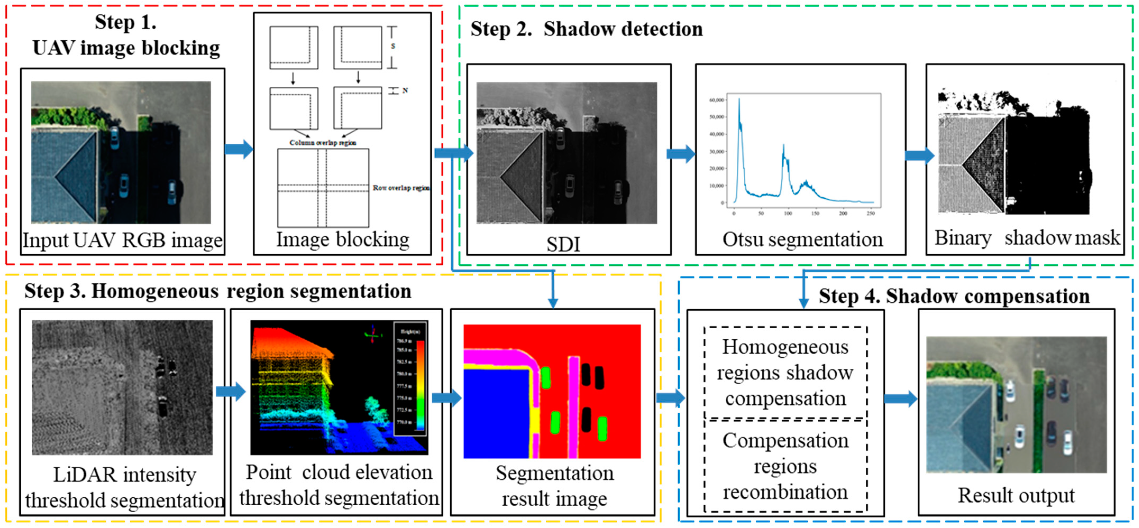
2. Methodology

The flowchart of the proposed methodology is shown in Figure 1. Firstly, the UAV imagery is split into blocks by selecting the size of the sliding window. Secondly, based on the red, green, and blue bands of UAV RGB image, a new shadow detection index (SDI) was defined to enhance the shadows. For the obtained SDI results, the shadow binary mask is obtained by using Otsu threshold segmentation and morphological optimization. Then, calculate the statistical characteristics of the LiDAR intensity and elevation for each image region, set segmentation threshold to extract homogeneous region. Finally, a shading compensation algorithm based on homogeneous region information is proposed, which can accurately recover the missing information in the shaded region by calculating the illumination ratio and grayscale difference between the shadow and non-shadow regions and using the homogeneous region entropy value to balance the color compensation and texture compensation.

2.1. UAV Image Blocking

UAV images are split into small blocks, which are used as the smallest processing unit in detecting shadow regions. In this process, an overlap area with an optimal size needs to be predetermined. A sliding window of size S × S is used to block the original remote sensing image, and S should be slightly larger than the length (L) or width (W) of the largest target on the study site. In this study, we suggest S = max(L,W) because it is common sense that the spectral information tends to be uniform in a small region. By using this way, inconsistency of restored objects and the objects without shadowing can be largely mitigated after shadow removal in an image. Meanwhile, in order to prevent unnaturally stitching objects which cover two adjacent blocks after shadow removal, an overlap region N is defined between these blocks, N = k × S (0 < k < 1), where k is the overlap rate of two adjacent blocks, and the value of parameter k can be flexibly selected based on the size of the block. A blocked image and the overlap regions are shown in Figure 2.

2.2. Shadow Detection

According to the analysis of color characteristics of UAV RGB remote sensing image [44], the red (R), green (G), and blue (B) components of the RGB color space are highly correlated (B-R: 0.78, R-G: 0.98, G-B: 0.94). Specifically, the reflectance of ground objects in the green band is slightly lower than that in the red band, and the red band of remote sensing images has high correlation with the green band; similarly, the reflectance of ground objects in the blue band is slightly lower than that in the green band, and the blue band of remote sensing images has high correlation with the green band. Subtraction operation can be used to increase the spectral reflectance between different ground objects and the contrast when the trend of change in the two bands is opposite. Woebbecke [45] analyzed $R-G$, $G-B$, $\left(G-B\right)/\left|R-G\right|$ and $2G-B-R$ optical characteristics, and found that $2G-B-R$ has the best optical contrast between the target and the background. According to the optical principle, the absorption band of a vegetation area is located in the blue band and red band, and the reflection peak is located in the green band. Light in non-shadow regions mainly comes from reflected light, ambient light, and atmospheric scattering. Light intensity perceived by sensors is mainly reflected light. Vegetation areas can strongly reflect green light. Therefore, the value of G component of the pixel corresponding to the vegetation area is larger than the value of the R and B components. By increasing the weight of the green component, the error detection of green vegetation can be eliminated.

Based on the above analysis, we propose a new shadow detection index (SDI) based on the red, green, and blue bands of a UAV RGB image, which is defined as follows:

$$\mathrm{SDI}=\mathsf{\omega }\times \left|2G-B-R\right|+\epsilon \times G$$

(1)

where, R, G, and B represent the red, green, and blue bands of the original UAV RGB image; ω, ε are parameters, and ω + ε = 1.

The Otsu method, also known as the maximum inter-class variance method, determines the threshold of binary image segmentation [46]. It divides the image into two parts, background and foreground. By calculating the inter-class variance of the foreground and background of each segmentation result, the gray value with the maximum inter-class variance is selected as the segmentation threshold. For the SDI, the Otsu method is used to extract the threshold of shadow segmentation automatically, and then the grayscale image was binarized to obtain the shadow mask. Then, the shadow mask is optimized by morphological operation.

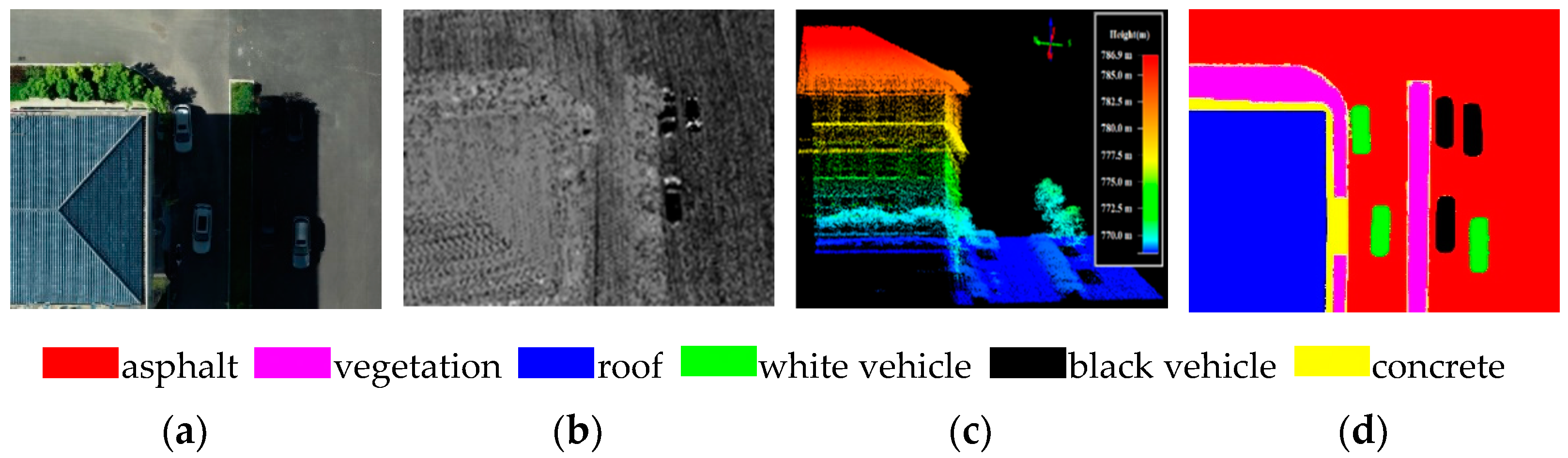
2.3. Homogeneous Region Segmentation

Shadow regions in an image may cover a variety of feature types, and the light reflectance of different surface materials varies. In developing the algorithm to restore color and texture details of shadowed regions, we take the difference into account. A homogeneous region is defined as a large connected region that is spatially adjacent and has the same or similar spectral properties, so that image pixels within it have strong spatial and spectral correlation [47]. In this process, we exploit high-resolution LiDAR point cloud and intensity data, acquired by a LiDAR device equipped with the UAV. LiDAR provides accurate elevation and intensity information that can be effectively associated in segmentation of homogeneous regions [48,49]. The algorithm can be described as follows:

(1)

Enhance the contrast of the intensity data using a histogram equalization method.

(2)

Calculate the statistical characteristics of the LiDAR intensity and elevation for each image region (each block).

(3)

A homogeneous region is selected using thresholding segmentation.

In the experiments of this study, ten types of homogeneous regions are defined and involved in the test images. They are asphalt road, concrete road, grassland, soil, tree, water, dark vehicle, white vehicle, roof, and rock. Region segmentation is performed by manually selecting the thresholding values based on a priori knowledge. For example, different intensity values (IN) and elevation values (EL) corresponding to different homogeneous regions in the image are shown in Figure 3. In Equation (2), and$IN{{\displaystyle \cap }}^{ }EL$ is a homogeneous region. An example result is shown in Figure 3d.

$$IN=\{\begin{array}{ll}0\le IN\le 10& Black metal\\ 30\le IN\le 60& Asphalt\\ 45\le IN\le 125& Vegetation\\ 120\le IN\le 200& Roof\\ 180\le IN\le 195& Concrete\\ 250\le IN\le 255& White metal\end{array}\hspace{1em}\hspace{1em}\hspace{1em}EL=\{\begin{array}{ll}0\le EL\le 0.3& Road\\ 1.3\le EL\le 2.2& Vehicle\\ 0.7\le EL\le 6.2& Tree\\ 4\le EL\le 18.8& Building\end{array}$$

(2)

2.4. Shadow Compensation

According to the image formation theory [50], the RGB values of image pixels conform to Equation (3).

$$I_i=L_i\times R_i$$

(3)

where $I_i$ is the RGB value at pixel point i, and $L_i$ and $R_i$ are the light intensity and surface reflectance of point i, respectively.

The imaging lighting effect can be regarded as a combination of direct light and ambient light, where direct light is the light that is shone directly from the light source to the object, and ambient light is the light that is obtained by reflection from other objects. Thus, for any pixel i, its intensity can be expressed as:

$$I_i^{}=\left(L_i^e+\alpha L_i^d\right)R_i,\alpha \in \left[0,1\right]$$

(4)

where, for pixel i, $L_i^e$ is the ambient light component, $L_i^d$ is the direct light component, and α is the shadow coefficient of the point. α = 1 means the pixel is not shaded; α = 0 refers to an object being fully shaded. In the transition region between fully shaded and unshaded regions, α is a continuous value and α ∈ (0,1).

The ratio of direct light to ambient light, r, can be expressed as:

$$r=\frac{I_i^{ns}- I_i^s}{ I_i^s}=\frac{\left(L_i^e+L_i^d\right)-\left(L_i^e+\alpha L_i^d\right)}{\left(L_i^e+\alpha L_i^d\right)}$$

(5)

In Equation (5), $I_i^{ns}$ represents pixel intensity at position i of a non-shadow image, and $I_i^s$ represents pixel intensity at position i of a shadow image.

Based on the above analysis, the intensity of a non-shadow pixel i can be expressed as:

$$I_i^{ns}=\frac{\left(r+1\right)}{\left(\alpha r+1\right)}{I}_i$$

(6)

As the light in the imaging area is completely or partially blocked by other obstacle objects, the brightness and contrast of the objects in the shadowed regions are reduced, which denotes the difference between the pixel values in the shadow or non-shadow regions. This difference is converted into a basis for effective enhancement of the shadow regions. For any shadow pixel i, the pixels after shadow compensation can be expressed as:

$$I_i^{s\_free}= I_i^s+d$$

(7)

In Equation (7), $I_i^{s\_free}$ is the shade-free pixel value and d is the difference between the average pixel value of the non-shadow and shadow regions.

$$d=\frac{1}{M}{\displaystyle \sum }_{i=1}^M I_i^{ns}-\frac{1}{N}{\displaystyle \sum }_{i=1}^N I_i^s$$

(8)

Illumination ratio-based shadow compensation methods are good at restoring texture information, but are prone to overcompensation and color distortion. Grayscale difference-based shadow compensation methods are good at restoring color information, but not suitable for shadow regions with complex textures. Combining the advantages and applicability conditions of the above two methods, the entropy value (ent) is used as the basis for judging which of the two methods is used for shadow compensation based on the complexity of the texture of the shadow regions.

$$ent=-{\displaystyle \sum }_{i=0}^n p\left(i\right){\log }_2\left[p\left(i\right)\right]$$

(9)

where n is all possible values of grayscale differential values and p(i) is the probability of each grayscale differential value.

The Algorithm 1 of shadow compensation is described as follows.

Algorithm 1. Shadow compensation algorithm

Input: UAV RGB image $I_j$$(j\in \left[1,m\right])$; The number of homogeneous regions, n; t. Output: The result of shadow compensation, $U^{removal}$, 1. All shadow regions are represented by S and all non-shadow regions are represented by U; 2. Find the non-shadow region $U_i$ corresponding to the homogeneous shadow region $S_i$, $i\in \left\{1,2,\cdot \cdot \cdot ,n\right\}$; 3. for (j = 1; j $\le$ m; j++) do 4.   for (i = 1; i $\le$ n; i ++) do 5.   compute the average value of $S_i$ in the q-band, $S_{i,q}^{avg}$ ($q\in \{R,G,B\}$); 6.   compute the average value of $U_i$ in the q-band, $U_{i,q}^{avg}$ ($q\in \{R,G,B\}$); 7.   $ent=-{\displaystyle {\displaystyle \sum }_{k=0}^N} p\left(k\right){\log }_2\left[p\left(k\right)\right]$; //the entropy value 8.    if (ent $\ge$  t) then 9.    $r_q=\frac{U_{i,q}^{avg}-S_{i,q}^{avg}}{S_{i,q}^{avg}}$; //the ratio of direct light to ambient light. 10.    $U_{i,q}^{removal}=\left(r_q+1\right)S_i$; //shadow compensation in the q-band. 11.   else 12.    $d_q=U_{i,q}^{avg}-S_{i,q}^{avg};$//the difference between the non-shadow and shadow regions. 13.    $U_{i,q}^{removal}=Si+d_q$;//shadow compensation in the q-band. 14.    end if 15.    $U_i^{removal}=\underset{q=R,G,B}{{\displaystyle \cup }}{U}_{i,q}^{removal}$;//the shadow compensation result of $S_i$ 16.   end for 17. end for 18. return $U^{removal}$;

3. Experiments

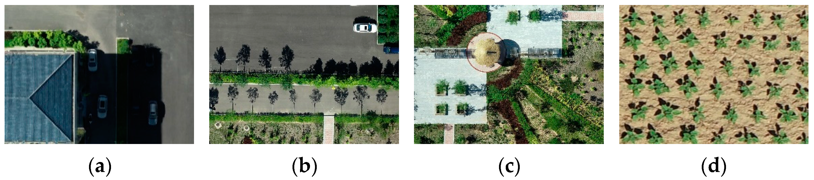
3.1. Experiment Data

Experiments were conducted with UAV images obtained by our team from aerial photography in Xinzhou City, Shanxi Province, China, with the longitude and latitude of 112°43′E and 38°27′N, and the UAV flight altitude was 85 m. The DJI “PHANTOM 4 RTK” drone is equipped with a CMOS camera of 20 effective megapixels and a maximum photo resolution of 5472 pixels × 3648 pixels (3:2). UAV images with complex surface features and a wide variety of objects were selected as experimental data, which contain multiple colors, textures, and a large amount of vegetation, asphalt roads, and concrete floors, as shown in Figure 4. The size of the image is 370 × 330 pixels in study case 4 (the fourth column in Figure 4), and the size of the other three images is 1500 × 1100 pixels. LiDAR data are obtained by DJI M600pro UAV with Genius LiDAR. The maximum range of this Genius Micro UAV-borne LiDAR is beyond 250 m, the maximum measurement speed is 640,000 points/second, and the actual operating point cloud density is better than 200 points/m². The system has a ranging accuracy of 2 cm and an absolute accuracy of better than 10 cm, which can satisfy topographic mapping work at a maximum scale of 1:500.

3.2. Experiment Design

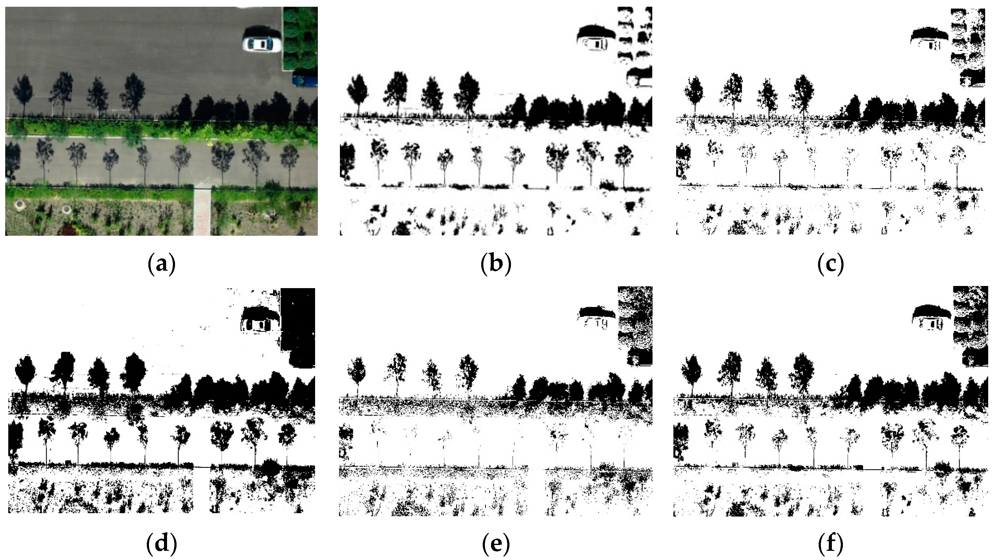
3.2.1. Experiment Design of Shadow Detection

To evaluate the proposed shadow detection algorithm, the experimental results are compared with the most commonly used shadow indexes, which are Tasi’s method in the YCbCr space (T_YCbCr) [25], Tasi’s method in the HSV space (T_HSV) [25], the normalized saturation-value difference index (NSVDI) [27], and the shadow index (SI) [26]. For objective evaluation, the producer’s accuracy (P_s and P_n), the user’s accuracy (U_s and U_n), the overall accuracy (OA), and F1 score are used.

$$\{\begin{array}{l}{P}_{\mathrm{s}}=\frac{TP}{TP+FN}\times 100\%\\ P_{\mathrm{n}}=\frac{TN}{TN+FP}\times 100\%\end{array}$$

(10)

$$\{\begin{array}{l}{U}_{\mathrm{s}}=\frac{TP}{TP+FP}\times 100\%\\ U_n=\frac{TN}{TN+FN}\times 100\%\end{array}$$

(11)

$$OA=\frac{TP+TN}{TP+TN+FP+FN}\times 100\%$$

(12)

$$F 1=2\times \frac{P_{\mathrm{s}}\times U_{\mathrm{s}}}{P_{\mathrm{s}}+U_{\mathrm{s}}}\times 100\%$$

(13)

where TP (true positive) is the number of shadow pixels correctly identified, TN (true negative) is the number of non-shadow pixels correctly identified, FP (false positive) is the number of non-shadow pixels incorrectly identified and FN (false negative) is the number of shadow pixels incorrectly identified. The closer the F1 score is to 1, the better is the performance of the shadow detection method.

3.2.2. Experiment Design of Shadow Compensation

To evaluate the proposed shadow compensation algorithm, the experimental results are compared with the most commonly used shadow compensation algorithms, which are the illumination correction method proposed by Silva [40], the color transfer method proposed by Murali [37], and the shadow synthesis method proposed by Inoue [11]. For objective evaluation, three metrics are used: (1) color difference (CD) for color consistency, (2) shadow standard deviation index (SSDI) proposed in [32] for texture detail consistency, and (3) gradient similarity (GS) for shadow boundary consistency.

(1)

Color difference (CD)

Convert images to the CIE L*a*b* color system with coordinates of a, b, L, using the CIE 1976L*a*b* color difference calculation Equation (14):

$$\mathsf{\Delta }{E}_{lab}={[{\left(\mathsf{\Delta }L\right)}^2+{\left(\mathsf{\Delta }a\right)}^2+{\left(\mathsf{\Delta }b\right)}^2]}^{1/2}$$

(14)

The relationship between color difference value and visual perception is:

When ∆E < 1, the chromatic aberration is barely perceived.

When 1 < ∆E ≤ 2, there is little perception of color difference.

When 2 < ∆E ≤ 3.5, the feeling of color difference is moderate.

When 3.5< ∆E ≤ 6, the feeling of color difference is obvious.

When ∆E > 6, the feeling of color difference is strong.

(2)

Shadow standard deviation index (SSDI)

The SSDI calculation is performed for each channel (R, G, and B) of the output image T, defined by ${\sigma }_{s-ns}$, as shown in Equation (15).

$${\sigma }_{s-ns}=\frac{1}{B}{\displaystyle \sum }_{b=1}^B\sqrt{\frac{1}{N}{\displaystyle \sum }_{i=1}^N{\left(F_{b,i}^s-\overline{F_b^{ns}}\right)}^2}$$

(15)

where b is the current band of the image and B is the total number of image bands. i is the current pixel in the shadow regions and N is the total number of pixels in the shadow regions. $F^s$ is the compensated shadow sample set, and $\overline{F^{ns}}$ is the mean of the corresponding non-shadow sample set.

The SSDI reflects the variation of the shadow regions after shadow compensation with regard to homogeneous non-shadow regions. When the SSDI value is low, it means the shadow regions are consistent with the non-shadow regions in terms of texture detail; when the SSDI value is high, it means the shadow regions are significantly different from the non-shadow regions in terms of texture detail.

(3)

Gradient similarity (GS)

$$g\left(x,y\right)=\frac{2g_x{g}_y+C}{g_x{}^2+g_y{}^2+C}$$

(16)

where $g_x$ and $g_y$ represent the central gradient values of image blocks x and y, respectively, and C is a smaller positive constant, in order to prevent the instability of the algorithm caused by too-small a denominator. $g\left(x,y\right)$ represents the x and y gradient similarity values, which ranges from 0 to 1.

3.3. Experimental Result

3.3.1. Experiment Result of Shadow Detection

Shadow detection results from the proposed method of the study cases 1 and 2 are shown in Figure 5 and Figure 6, in comparison with the other four aforementioned methods. Study case 1 contains large and regular building shadows. Study case 2 contains a lot of irregular and fragmented tree shadows. The results of all five methods in terms of detection accuracy in study cases 1 and 2 are shown in

Table 1. Objective evaluation results of shadow detection in study case 1.

Index	Ps (%)	Pn (%)	Us (%)	Un (%)	OA (%)	F1 (%)
SDI	98.09	99.50	99.22	98.75	98.94	98.65
TYCbCr	81.40	99.60	99.40	87.00	91.51	89.50
THSV	99.69	79.28	79.38	99.68	88.35	88.38
NSVDI	80.33	98.54	97.77	86.23	90.45	88.20
SI	86.84	99.47	99.24	90.43	93.85	92.62

and

Table 2. Objective evaluation results of shadow detection in study case 2.

Index	Ps (%)	Pn (%)	Us (%)	Un (%)	OA (%)	F1 (%)
SDI	94.00	98.27	92.08	98.71	97.51	93.03
TYCbCr	75.51	98.45	90.16	95.53	94.82	82.19
THSV	98.13	84.62	54.56	99.59	86.76	70.13
NSVDI	63.13	93.82	65.28	93.12	88.96	64.43
SI	90.55	95.73	79.98	98.18	94.91	84.94

, respectively.

3.3.2. Experiment Result of Shadow Detection

Shadow compensation results from the proposed method of the four study cases are shown in Figure 7, in comparison with the other three aforementioned methods. In addition, the compensation results of each method are locally enlarged to observe the details of feature information recovery under shadows, as shown in Figure 8. The results of all four methods in terms of compensation accuracy in each study case are shown in

Table 3. Objective evaluation results of color difference (CD).

Case	Illumination Correction	Color Transfer	Shadow Synthesis	Proposed Work
1	4.863	4.352	2.936	1.792
2	4.340	4.053	3.902	1.943
3	5.654	4.924	4.761	1.831
4	5.207	3.896	3.632	1.998
AVG	5.016	4.306	3.807	1.891

,

Table 4. Objective evaluation results of shadow standard deviation index (SSDI).

Case	Illumination Correction	Color Transfer	Shadow Synthesis	Proposed Work
1	23.326	22.013	16.877	16.509
2	19.872	20.362	19.843	17.182
3	18.439	19.394	18.160	13.731
4	18.310	19.212	15.485	14.253
AVG	19.896	20.245	17.591	15.419

and

Table 5. Objective evaluation results of gradient similarity (GS).

Case	Illumination Correction	Color Transfer	Shadow Synthesis	Proposed Work
1	0.491	0.574	0.718	0.769
2	0.503	0.519	0.582	0.673
3	0.464	0.483	0.603	0.721
4	0.510	0.521	0.596	0.740
AVG	0.492	0.524	0.625	0.726

, respectively.

4. Discussion

4.1. Sensitivity of Parameter Settings

In Section 2.1, we introduced a parameter k in image blocking. In Section 2.2, we introduced parameters ω and ε in shadow detection. Due to the sensitivity of the parameter setting, we analyze the influence of overlap rate k on the consistency of feature information recovery at the stage of image stitching by adjusting the value of parameter k. Furthermore, we analyze the effect of the parameters including ω and ε (ω + ε = 1) on the performance of the shadow detection algorithm.

The Kappa coefficient is selected as the consistency test and detection accuracy index. The relationship between the Kappa coefficient and parameters k and ω is shown in Figure 9. The range of k is chosen from 0 to 0.7, the range of ω is chosen from 0.1 to 0.9, and the step interval is 0.1, which shows that the size of the parameters including k, ω, and ε has a significant influence on the Kappa coefficient. The four typical study cases as discussed in Section 3.1 are selected for the analysis. The Kappa coefficient curves in Figure 9a,b show the same trend in the four study cases. It is found that k has an influence on the Kappa coefficient, and k = 0.2 might be a good setting for almost all cases. As presented in Figure 9b, when $\omega \in \left(0.1,0.3\right)$, relatively higher Kappa coefficient values are acquired for the four study cases, which shows that better shadow detection results are achieved. This further demonstrates the robustness and effectiveness of the proposed method under different various landscapes. Hence, in this study, we develop the shadow compensation approach over study cases with k = 0.2 and ω = 0.2.

In Section 2.4, we introduced a threshold value t in the shadow compensation algorithm. It was found that the entropy values of homogeneous regions in UAV remote sensing images range from 3 to 8. When t < 5.3, the texture of the compensated shadow regions is clear, but the color information is lost. When t > 5.8, the color of the compensated shadow regions is correctly corrected, but the texture is blurred. When 5.3 < t < 5.8, both texture and color information in the shadow region are recovered optimally. In the experiment of this paper, t is taken as 5.5.

4.2. Analysis of Experimental Results of Shadow Detection

4.2.1. Subjective Evaluation and Discussion

As shown in Figure 5, there is a large area of building shadow in study case 1. The result of the method proposed in this study is shown in Figure 5b. It can be seen that the method obtained satisfactory results. T_YCbCr identifies the high-reflectance ground object pixels (white vehicles) in the shadow region as non-shadow pixels, which causes omission errors. T_HSV is unable to remove the interference of plants and artificially colored ground objects to the shadow. As shown in Figure 5d, the pixels of some blue roofs, dark green vegetation, and sporadic ground points are mistakenly detected as shadows pixels. NSVDI also causes omission errors, as shown in Figure 5e. This is because the HSV space is restricted by the fact that when the pixel values in R, G, and B bands are equal, the denominator of the HSV’s definition is 0, generating invalid values. Similarly, SI is also susceptible to the influence of high-reflectance ground objects and mistakenly identifies white vehicle pixels in the shadow region as non-shadow pixels, as shown in Figure 5f.

As shown in Figure 6, there are a large number of irregular fragmented tree shadows in study case 2. The result of the method proposed in this study is shown in Figure 6b, showing good integrity of shadow detection. The results of T_YCbCr, NSVDI, and SI were similar. It can be seen that the extraction of the tree shadow edge is incomplete, and pixels of the shadow edge are missed, and a small number of dark green vegetation pixels are detected as shadow pixels. As the gray value of the region is close to the gray value of vegetation pixels, as shown in Figure 6d, the tree shadow is not correctly detected, and T_HSV mistakenly detects most vegetation pixels as shadow pixels.

4.2.2. Objective Evaluation and Discussion

As shown in Table 1, relatively high values are achieved for shadow detection results by the SDI method proposed in this study for the study case 1 in terms of the shadow producer’s accuracy (98.09%), the shadow user’s accuracy (99.22%), the non-shadow producer’s accuracy (99.50%), and the non-shadow user’s accuracy (98.75%). The overall accuracy is up to 98.94% and the F1 score is up to 98.65%, which are higher than the T_YCbCr, T_HSV, NSVDI, and SI methods. This proves that our method has fewer omissions and false detections.

Similarly, as shown in Table 2, relatively high and stable values are also obtained for shadow detection results by the SDI method proposed in this study for the study case 2 in terms of the shadow producer’s accuracy (94.00%), the shadow user’s accuracy (92.08%), the non-shadow producer’s accuracy (98.27%), and the non-shadow user’s accuracy (98.71%). The overall accuracy is 97.51% and the F1 score is 93.03%, which are higher than the other four methods. In general, SDI provides relatively ideal and stable shadow detection accuracy measurements in both experimental sites.

4.3. Analysis of Experimental Results of Shadow Compensation

4.3.1. Subjective Evaluation and Discussion

The first column in Figure 7 is the result of study case 1. It can be seen that the illumination correction algorithm cannot recover the color information accurately when large building shadows cover the asphalt road, although the texture details of the shadow regions are preserved. The color transfer algorithm tends to keep the blue color. In addition, the vehicles and vegetation areas are blurred. The shadow synthesis method results in smoother boundaries than the previous two methods, but there is still obvious difference between shadow and non-shadow regions with regards to color. In contrast, the method proposed in this study provides better visual consistency in the color of the asphalt areas after the shadow compensation process, although the boundaries are still visible. In addition, it is notable that the vegetation areas retain texture information and the vehicles are clearly restored. However, due to the uneven distribution of illumination on the side facade of the roof and the influence of image block effect, the proposed method produces a blocky artifact within the roof. In this regard, the proposed method failed to present a good recovery effect completely.

The second column in Figure 7 is the result of study case 2, when irregular vegetation shadows cover the asphalt road, the green vegetation area after applying the illumination correction algorithm is over-illuminated, and there is oversaturation in the transition area between shadow and non-shadow regions. The asphalt area after compensation by the color transfer algorithm presents color inconsistency at the shadow boundary, whilst the shadow region after compensation by the shadow synthesis method becomes green, the color and texture information are visually inconsistent, and the texture information of the green vegetation area is blurred. The results obtained using our method show that the color of the asphalt area is improved after shadow compensation compared with the other three methods, and the texture and color of the green vegetation are closer to the real scenery.

The third column in Figure 7 is the result of study case 3. When shadow compensation happens in concrete areas, the illumination correction algorithm and the color transfer algorithm tend to maintain the blue-like color. The shadow synthesis method provides a result with color closer to that of the non-shadow regions, but the vegetation after shadow compensation still has significant difference in texture details, as shown in Figure 8. The proposed method significantly improves the color inconsistency, and the shadow boundaries are not as obvious as those from other methods. In addition, the vegetation after shadow compensation has obvious improvement in texture details.

The fourth column in Figure 7 is the result of study case 4. When compensating the shadows of sunflower plants in farmland, both the illumination correction algorithm and the color transfer algorithm leave a clear boundary effect between the shadow and non-shadow regions after the shadow compensation process. The shadow synthesis method and the proposed method have both achieved more satisfactory results with regards to the boundary effect, but the shadow synthesis method did not recover the objects (two cars) in the shadowed region, as shown in Figure 8.

4.3.2. Objective Evaluation and Discussion

Table 3 shows the results of color difference calculated by Equation (14) for all shadow compensation methods. The CD values of our method for four experimental images are 1.792, 1.943, 1.831, and 1.998, with an average CD value of 1.891. In contrast, the average CD value is 3.125, 2.415, and 1.916 for the illumination correction, the color transfer and shadow synthesis methods, respectively. This proves that our method has less color distortion after shadow compensation.

The SSDI results are presented in Table 4, and the SSDI values of our method are 16.509, 17.182, 13.731, and 14.253 for the four experimental images, respectively, with an average SSDI value of 15.419. Compared with the average SSDI values from the illumination correction and the color transfer methods, it is 4.477 and 4.826 lower. The average SSDI value from our method is numerically 2.172 lower than that of the shadow synthesis method. This means that our method produces good results, in which the compensated shadow regions and non-shadow regions are consistent in terms of texture details.

Table 5 gives the results of the gradient similarity of all methods for the four test images. The shaded boundary GS values for our method are 0.769, 0.673, 0.721, and 0.740 for the four test images, respectively, with an average of 0.726. It is 0.234, 0.202, and 0.101 higher than the average shaded boundary GS values of the illumination correction, the color transfer and shadow synthesis methods, respectively.

Based on the above analysis, the combination of LiDAR information and UAV visible images in this study leads to a better result. When designing the homogeneous area segmentation method based on the information of LiDAR intensity and elevation, we defined the intensity range and elevation range of typical features based on a priori knowledge and rigorous statistical analysis. The threshold range is applicable to most scenes and has strong universality. In addition, in terms of data acquisition, it is certainly more universal if only a single device is used for testing, but the accuracy needs to be improved.

5. Conclusions

In this study, we have presented a shadow removal method from UAV images based on color and texture equalization compensation of local homogeneous regions. The following conclusions are drawn through comparative analysis of the experimental results.

(1)

The new shadow detection index, defined based on the R, G, and B bands of a UAV image, can effectively enhance the shadow, and is conducive to accurate shadow extraction of UAV RGB remote sensing images. The average overall accuracy of shadow detection is 98.23% and the average F1 score is 95.84%.

(2)

The proposed method was tested in scenes containing quite complex surface features and a great variety of objects, and it performed well. In the visual effect, the color and texture details of the shadow regions are effectively compensated, and the shadow border is not obvious. The compensated image had high consistency with the real scenes. Likewise, in the quantitative analysis, the average color difference is 1.891, the average shadow standard deviation index is 15.419, and the average gradient similarity is 0.726. It achieved the best results compared with the aforementioned testing methods and proved the effectiveness of the proposed method.

In the future, the work may extend to optimizing homogeneous region segmentation and processing shadow boundaries.

References

- Adeline, K.; Chen, M.; Briottet, X.; Pang, S.K.; Paparoditis, N. Shadow detection in very high spatial resolution aerial images: A comparative study. ISPRS J. Photogramm. Remote Sens. Environ. 2013, 80, 21–38. [Google Scholar] [CrossRef]
- Zhou, W.; Huang, G.; Troy, A.; Cadenasso, M.L. Object-based land cover classification of shaded areas in high spatial resolution imagery of urban areas: A comparison study. Remote Sens. Environ. 2009, 113, 1769–1777. [Google Scholar] [CrossRef]
- Ankush, A.; Kumar, S.; Singh, D. An Adaptive Technique to Detect and Remove Shadow from Drone Data. J. Indian Soc. Remote 2021, 49, 491–498. [Google Scholar]
- Amin, B.; Riaz, M.M.; Ghafoor, A. Automatic shadow detection and removal using image matting. Signal Processing 2019, 170, 107415. [Google Scholar] [CrossRef]
- Arévalo, V.; González, J.; Ambrosio, G. Shadow detection in colour high-resolution satellite images. Int. J. Remote Sens. 2008, 29, 1945–1963. [Google Scholar] [CrossRef]
- Mostafa, Y.; Abdelwahab, M.A. Corresponding regions for shadow restoration in satellite high-resolution images. Int. J. Remote Sens. 2018, 39, 7014–7028. [Google Scholar] [CrossRef]
- Gao, M.; Yang, F.; Wei, H.; Liu, X. Individual Maize Location and Height Estimation in Field from UAV-Borne LiDAR and RGB Images. Remote Sens. 2022, 14, 2292. [Google Scholar] [CrossRef]
- Zhang, Y.; Chen, G.; Vukomanovic, J.; Singh, K.; Liu, Y.; Holden, S.; Meentemeyer, R.K. Recurrent Shadow Attention Model (RSAM) for shadow removal in high-resolution urban land-cover mapping. Remote Sens. Environ. 2020, 247, 111945. [Google Scholar] [CrossRef]
- Luo, Y.; Xin, J.; He, H.; Geomatics, F.O. Research on shadow detection method of WorldView-Ⅱremote sensing image. Sci. Surv. Mapp. 2017, 42, 132–142. [Google Scholar]
- Wen, Z.; Wu, S.; Chen, J.; Lyu, M.; Jiang, Y. Radiance transfer process based shadow correction method for urban regions in high spatial resolution image. J. Remote Sens. 2016, 20, 138–148. [Google Scholar]
- Inoue, N.; Yamasaki, T. Learning from Synthetic Shadows for Shadow Detection and Removal. IEEE Trans. Circuits Syst. Video Technol. 2021, 31, 4187–4197. [Google Scholar] [CrossRef]
- Gilberto, A.; Roque, A.O.; Francisco, J.S.; Luis, L. An Approach for Shadow Detection in Aerial Images Based on Multi-Channel Statistics. IEEE Access 2021, 9, 34240–34250. [Google Scholar]
- Han, H.; Han, C.; Lan, T.; Huang, L.; Hu, C.; Xue, X. Automatic Shadow Detection for Multispectral Satellite Remote Sensing Images in Invariant Color Spaces. Appl. Sci. 2020, 10, 6467. [Google Scholar] [CrossRef]
- Luo, H.; Shao, Z. A Shadow Detection Method from Urban High Resolution Remote Sensing Image Based on Color Features of Shadow. In Proceedings of the International Symposium on Information Science and Engineering (ISISE), Shanghai, China, 14–16 December 2012; pp. 48–51. [Google Scholar]
- Liu, Y.; Wei, Y.; Tao, S.; Dai, Q.; Wang, W.; Wu, M. Object-oriented detection of building shadow in TripleSat-2 remote sensing imagery. J. Appl. Remote Sens. 2020, 14, 036508. [Google Scholar] [CrossRef]
- Bendig, J.; Bolten, A.; Bennertz, S.; Broscheit, J.; Eichfuss, S.; Bareth, G. Estimating Biomass of Barley Using Crop Surface Models (CSMs) Derived from UAV-Based RGB Imaging. Remote Sens. 2014, 6, 10395–10412. [Google Scholar] [CrossRef] [Green Version]
- Duan, G.; Gong, H.; Li, X.; Chen, B. Shadow extraction based on characteristic components and object-oriented method for high-resolution images. J. Appl. Remote Sens. 2014, 18, 760–778. [Google Scholar]
- Zhang, H.; Sun, K.; Li, W. Object-Oriented Shadow Detection and Removal from Urban High-Resolution Remote Sensing Images. IEEE Trans. Geosci. Remote Sens. Lett. 2014, 52, 6972–6982. [Google Scholar] [CrossRef]
- Ehlem, Z.; Mohammed, F.B.; Mohammed, K.; Mohammed, D.; Belkacem, K. New shadow detection and removal approach to improve neural stereo correspondence of dense urban VHR remote sensing images. Eur. J. Remote Sens. 2015, 48, 447–463. [Google Scholar]
- Luo, H.; Wang, L.; Shao, Z.; Li, D. Development of a multi-scale object-based shadow detection method for high spatial resolution image. Remote Sens. Lett. 2015, 6, 59–68. [Google Scholar] [CrossRef]
- Tolt, G.; Shimoni, M.; Ahlberg, J. A shadow detection method for remote sensing images using VHR hyperspectral and LIDAR data. In Proceedings of the International Geoscience and Remote Sensing Symposium, Vancouver, BC, Canada, 24–29 July 2011; pp. 4423–4426. [Google Scholar]
- Liu, X.; Hou, Z.; Shi, Z.; Bo, Y.; Cheng, J. A shadow identification method using vegetation indices derived from hyperspectral data. Int. J. Remote Sens. 2017, 38, 5357–5373. [Google Scholar] [CrossRef]
- Shao, Q.; Xu, C.; Zhou, Y.; Dong, H. Cast shadow detection based on the YCbCr color space and topological cuts. J. Supercomput. 2020, 76, 3308–3326. [Google Scholar] [CrossRef]
- Sun, G.; Huang, H.; Weng, Q.; Zhang, A.; Jia, X.; Ren, J.; Sun, L.; Chen, X. Combinational shadow index for building shadow extraction in urban areas from Sentinel-2A MSI imagery. Int. J. Appl. Earth Obs. Geoinf. 2019, 78, 53–65. [Google Scholar] [CrossRef]
- Tsai, V.J.D. A comparative study on shadow compensation of color aerial images in invariant color models. IEEE Trans. Geosci. Remote Sens. Lett. 2006, 44, 1661–1671. [Google Scholar] [CrossRef]
- Zhou, T.; Fu, H.; Sun, C. Shadow Detection and Compensation from Remote Sensing Images under Complex Urban Conditions. Remote Sens. 2021, 13, 699. [Google Scholar] [CrossRef]
- Ma, H.; Qin, Q.; Shen, X. Shadow Segmentation and Compensation in High Resolution Satellite Images. In Proceedings of the International Geoscience and Remote Sensing Symposium, Boston, MA, USA, 7–11 July 2008; pp. 1036–1039. [Google Scholar]
- Wen, Z.; Shao, G.; Mirza, Z.A.; Chen, J.; Lu, M.; Wu, S. Restoration of shadows in multispectral imagery using surface reflectance relationships with nearby similar areas. Int. J. Remote Sens. 2015, 36, 4195–4212. [Google Scholar] [CrossRef]
- Mostafa, Y. A Review on Various Shadow Detection and Compensation Techniques in Remote Sensing Images. Can. J. Remote Sens. 2017, 43, 545–562. [Google Scholar] [CrossRef]
- Zhang, L.; Zhang, Q.; Xiao, C. Shadow Remover: Image Shadow Removal Based on Illumination Recovering Optimization. IEEE Trans. Image Processing 2015, 24, 4623–4636. [Google Scholar] [CrossRef]
- Mo, N.; Zhu, R.; Yan, L.; Zhao, Z. Deshadowing of Urban Airborne Imagery Based on Object-Oriented Automatic Shadow Detection and Regional Matching Compensation. IEEE J. Sel. Top. Appl. Earth Obs. Remote Sens. 2018, 11, 585–605. [Google Scholar] [CrossRef]
- Luo, S.; Shen, H.; Li, H.; Chen, Y. Shadow removal based on separated illumination correction for urban aerial remote sensing images. Signal Processing 2019, 165, 197–208. [Google Scholar] [CrossRef]
- Shahtahmassebi, A.; Yang, N.; Wang, K.; Moore, N.; Shen, Z. Review of shadow detection and de-shadowing methods in remote sensing. Chin. Geogr. Sci. 2013, 23, 403–420. [Google Scholar] [CrossRef] [Green Version]
- Sabri, M.A.; Aqel, S.; Aarab, A. A multiscale based approach for automatic shadow detection and removal in natural images. Multimed. Tools Appl. 2019, 78, 11263–11275. [Google Scholar] [CrossRef]
- Su, N.; Zhang, Y.; Tian, S.; Yan, Y.; Miao, X. Shadow Detection and Removal for Occluded Object Information Recovery in Urban High-Resolution Panchromatic Satellite Images. IEEE J. Sel. Top. Appl. Earth Obs. Remote Sens. 2016, 9, 2568–2582. [Google Scholar] [CrossRef]
- Yago, V.T.F.; Hoai, M.; Samaras, D. Leave-one-out kernel optimization for shadow detection and removal. IEEE Trans. Pattern Anal. Mach. Intell. 2018, 40, 682–695. [Google Scholar]
- Saritha, M.; Govindan, V.K. Shadow Detection and Removal from a Single Image Using LAB Color Space. Cybern. Inf. Technol. 2013, 13, 95–103. [Google Scholar]
- Jian, Y.; Yu, H.; John, C. Fully constrained linear spectral unmixing based global shadow compensation for high resolution satellite imagery of urban areas. Int. J. Appl. Earth Obs. Geoinf. 2015, 38, 88–98. [Google Scholar]
- Song, H.; Huang, B.; Zhang, K. Shadow Detection and Reconstruction in High-Resolution Satellite Images via Morphological Filtering and Example-Based Learning. IEEE Trans. Geosci. Remote Sens. 2014, 52, 2545–2554. [Google Scholar] [CrossRef]
- Silva, G.F.; Carneiro, G.B.; Doth, R.; Amaral, L.A.; De Azevedo, D.F.G. Near real-time shadow detection and removal in aerial motion imagery application. ISPRS J. Photogramm. Remote Sens. Lett. 2017, 140, 104–121. [Google Scholar] [CrossRef]
- Gilberto, A.; Francisco, J.S.; Marco, A.G.; Roque, A.O.; Luis, A.M. A Novel Shadow Removal Method Based upon Color Transfer and Color Tuning in UAV Imaging. Appl. Sci. 2021, 11, 11494. [Google Scholar]
- Awad, M.M. Toward Robust Segmentation Results Based on Fusion Methods for Very High Resolution Optical Image and LiDAR Data. IEEE J. Sel. Top. Appl. Earth Obs. Remote Sens. 2017, 10, 2067–2076. [Google Scholar] [CrossRef]
- Han, X.; Wang, H.; Lu, J.; Zhao, C. Road detection based on the fusion of Lidar and image data. Int. J. Adv. Robot. Syst. 2017, 14, 1. [Google Scholar] [CrossRef] [Green Version]
- Liu, J.; Yang, J.; Fang, T. Color Property Analysis of Remote Sensing Imagery. Acta Photonica Sin. 2009, 38, 441–447. [Google Scholar]
- Woebbecke, D.M.; Meyer, G.E.; Bargen, K.V.; Mortensen, D.A. Color indices for weed identification under various soil, residual, and lighting conditions. Trans. ASAE 1995, 38, 259–269. [Google Scholar] [CrossRef]
- Otsu, N. A Threshold Selection Method from Gray-Level Histograms. IEEE Trans. Syst. Man Cybern. 1979, 9, 62–66. [Google Scholar] [CrossRef] [Green Version]
- Wanderson, S.C.; Leila, M.G.F.; Thales, S.K.; Margareth, S.; Hugo, N.B.; Ricardo, C.M.S. Segmentation of Optical Remote Sensing Images for Detecting Homogeneous Regions in Space and Time. Rev. Bras. Cartogr. 2018, 70, 1779–1801. [Google Scholar]
- Yang, F.; Wei, H.; Feng, P. A hierarchical Dempster-Shafer evidence combination framework for urban area land cover classification. Measurement 2020, 151, 105916. [Google Scholar] [CrossRef]
- Feng, P.; Yang, F.; Wei, H. A fast method for land-cover classification from LIDAR data based on hybrid Dezert-Smarandache Model. ICIC Express Lett. Part B Appl. 2015, 6, 3109–3114. [Google Scholar]
- Barrow, H.; Tenenbaum, J.; Hanson, A.; Riseman, E. Recovering intrinsic scene characteristics. Comput. Vis. Syst. 1978, 2, 2. [Google Scholar]