
New Insights into Ice Avalanche-Induced Debris Flows in Southeastern Tibet Using SAR Technology


 , ,
, ,  ,
,
Abstract
:1. Introduction
2. Study Area and Data Sources
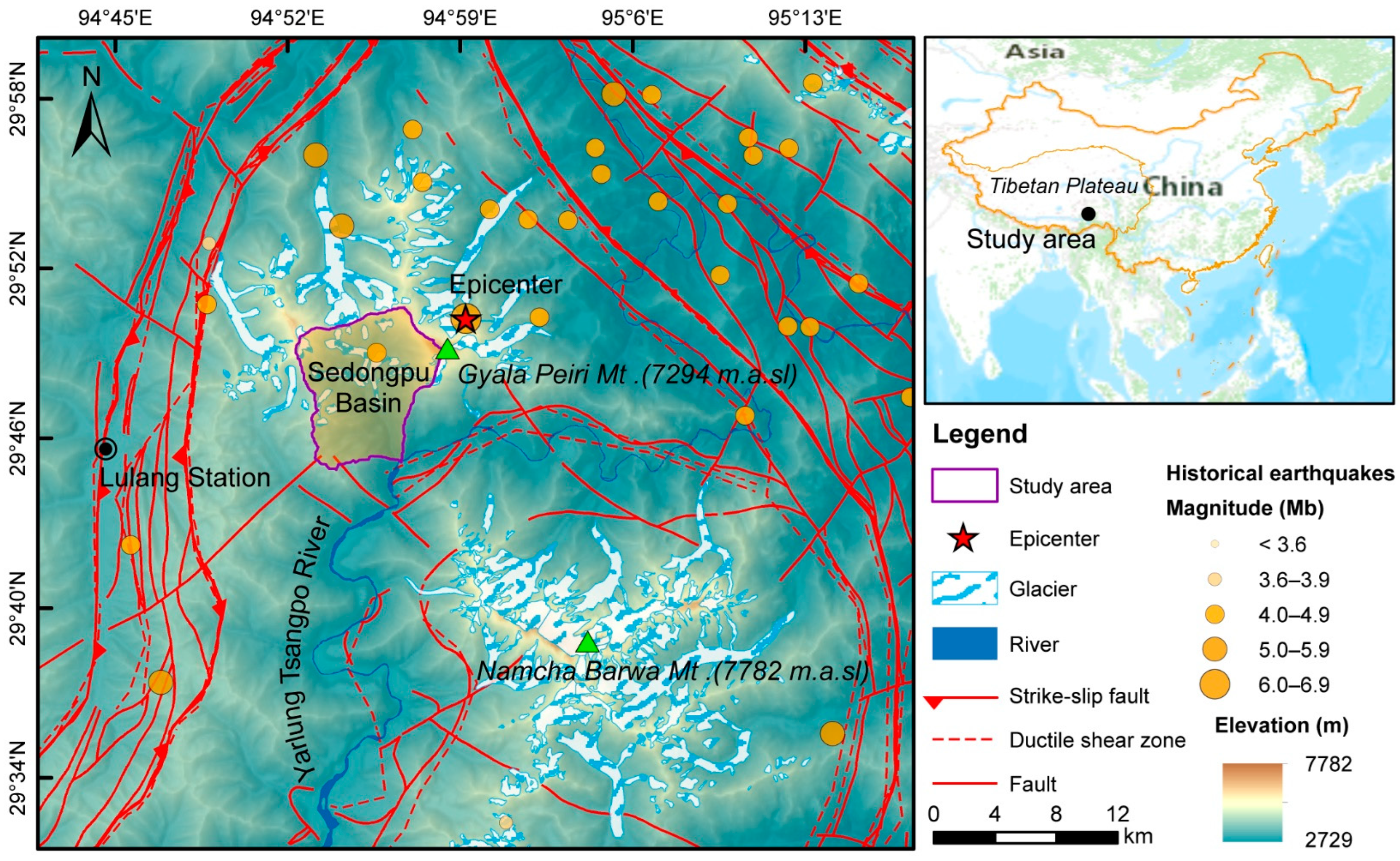
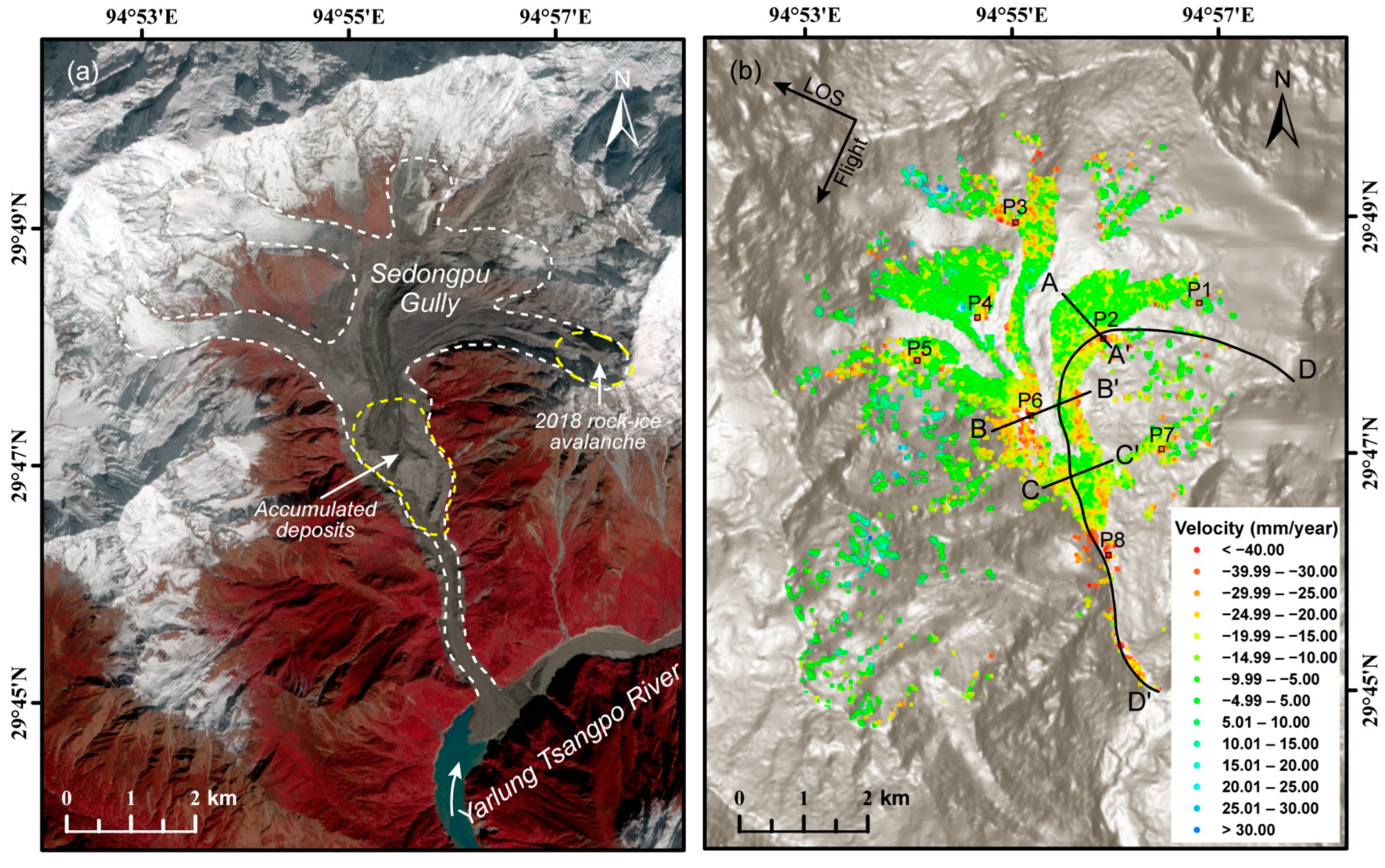
2.1. Study Area
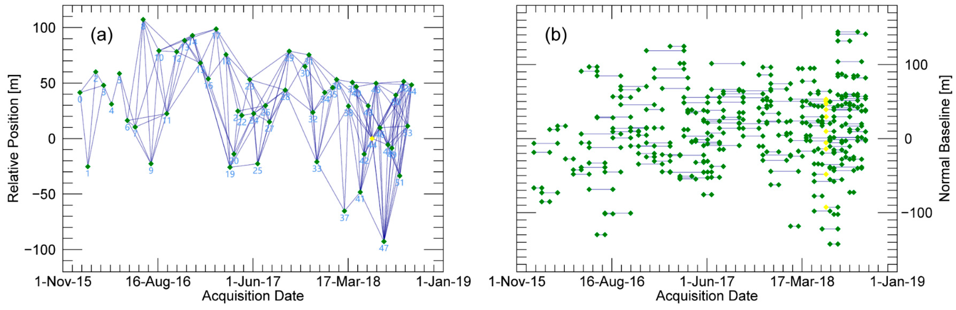
2.2. Data Sources
3. Methodology
3.1. Fundamental Principle of the SBAS Method
3.2. Extraction of Wet Snow Cover Area
4. Results and Analysis
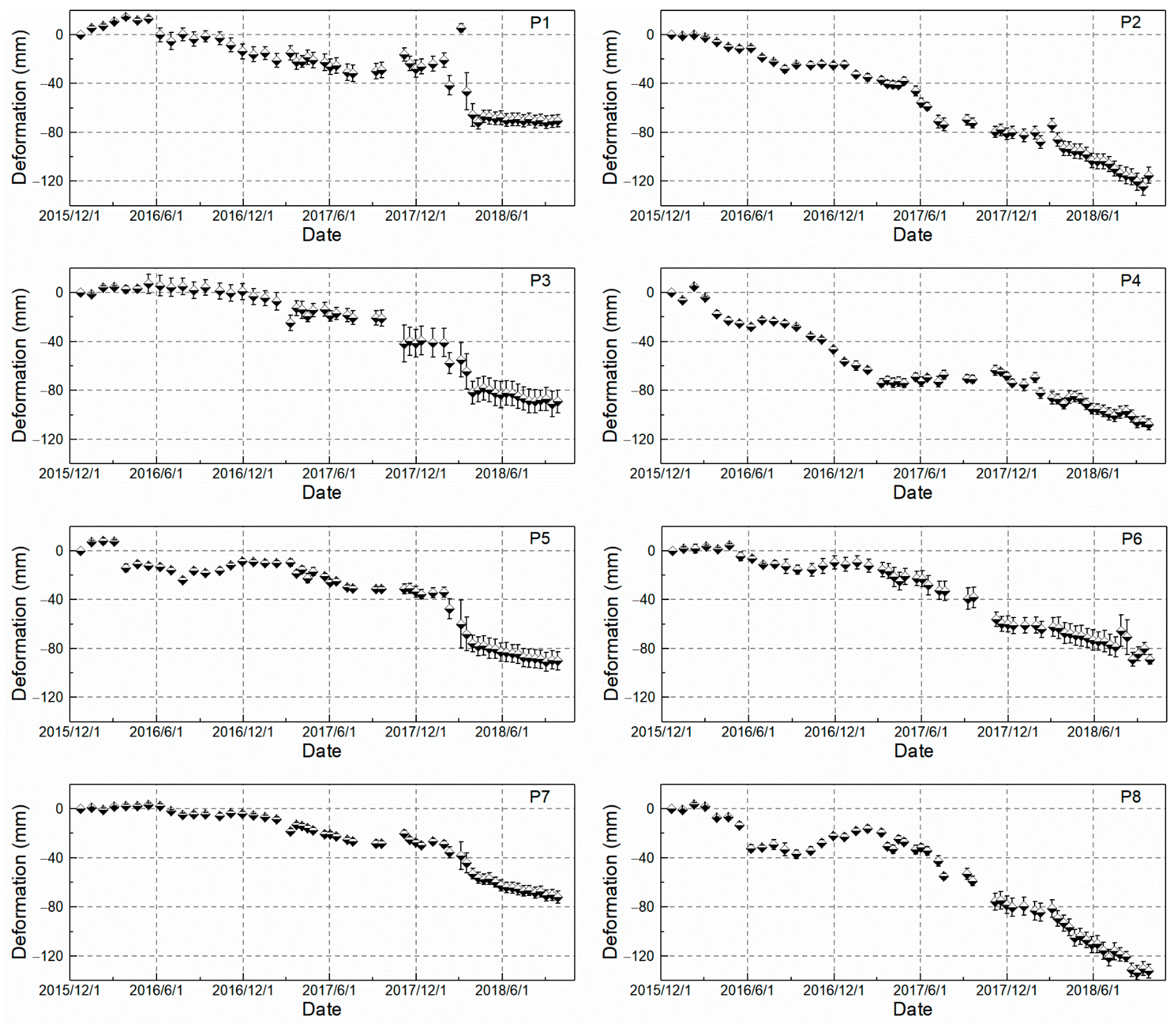
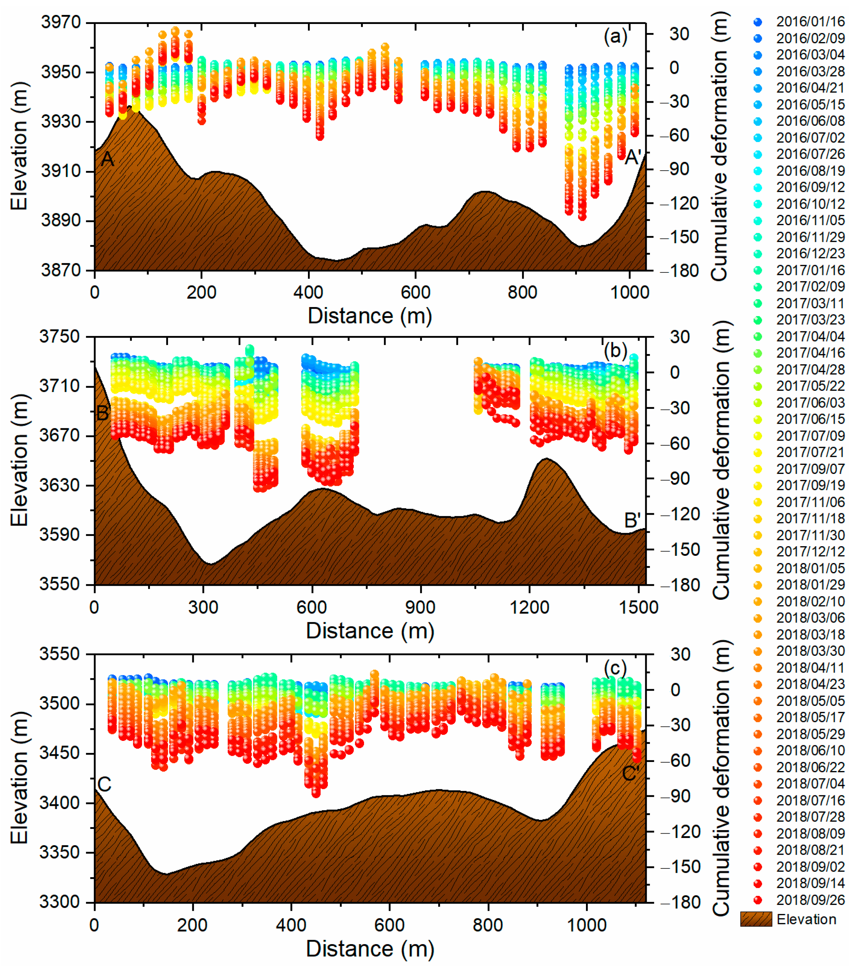
4.1. Precursory Movements of Ice Avalanche-Induced Debris Flows Measured via Time Series InSAR Analysis
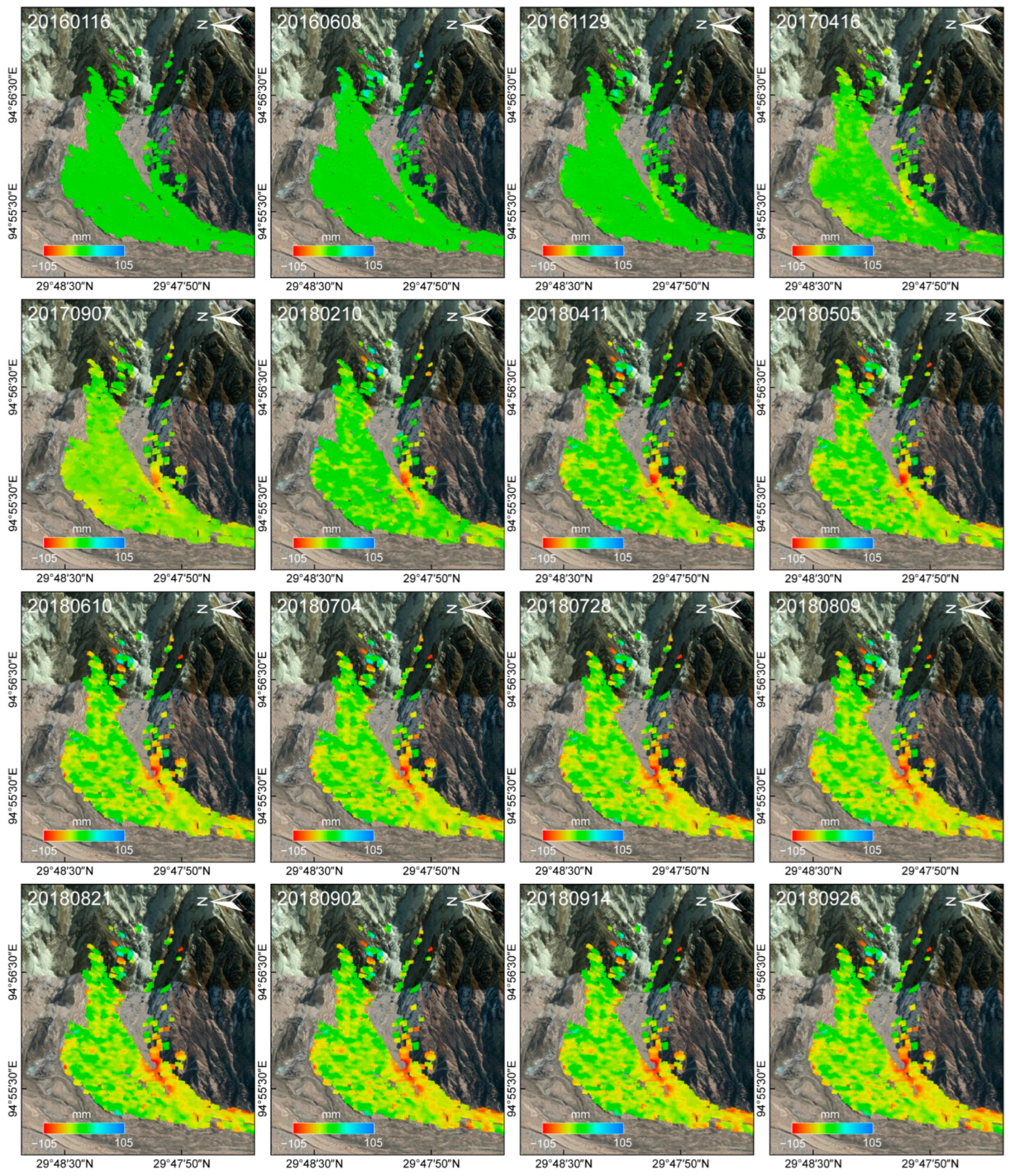
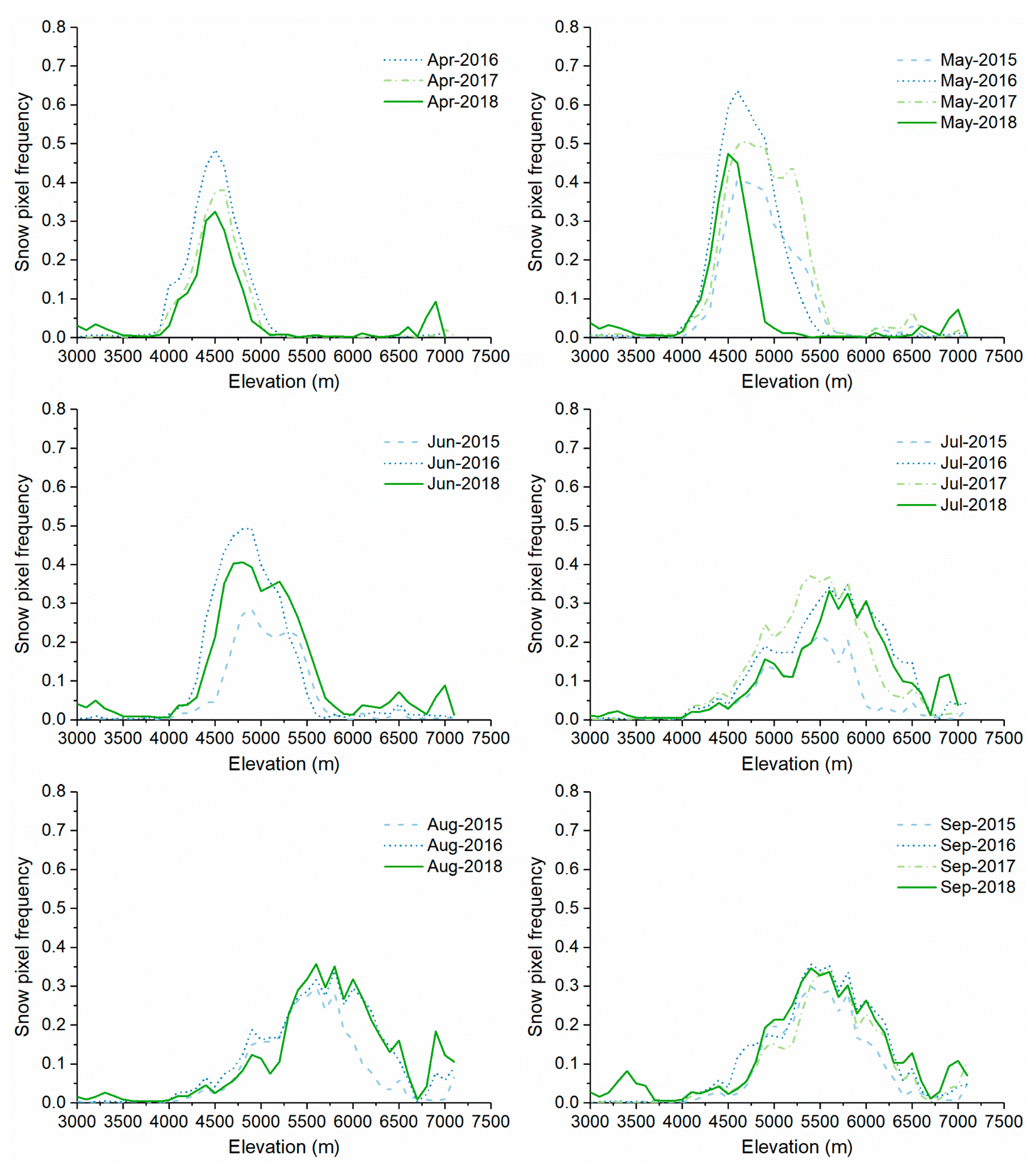
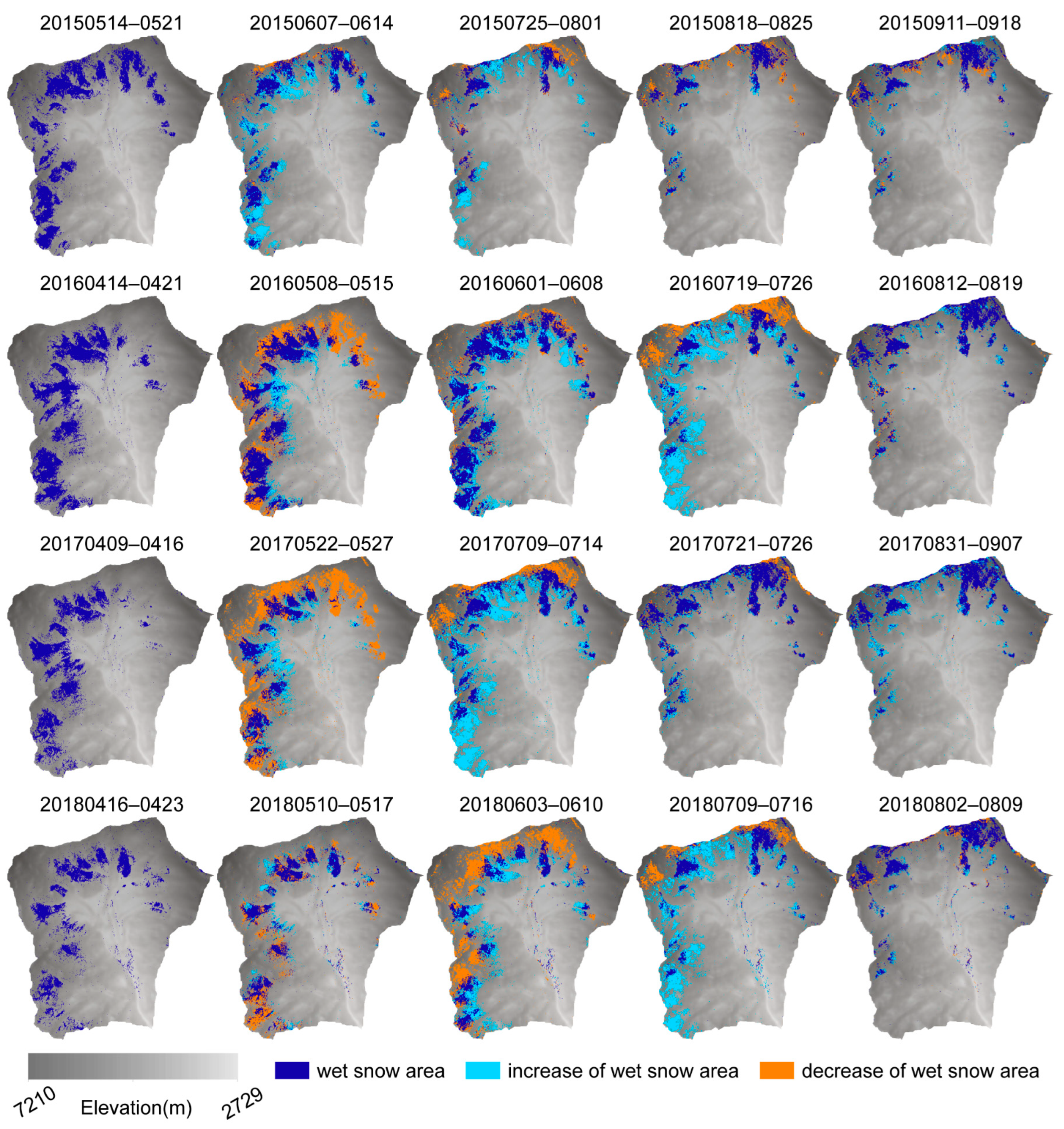
4.2. Spatiotemporal Changes in the Wet Snow Area during the Snowmelt Season
5. Discussion
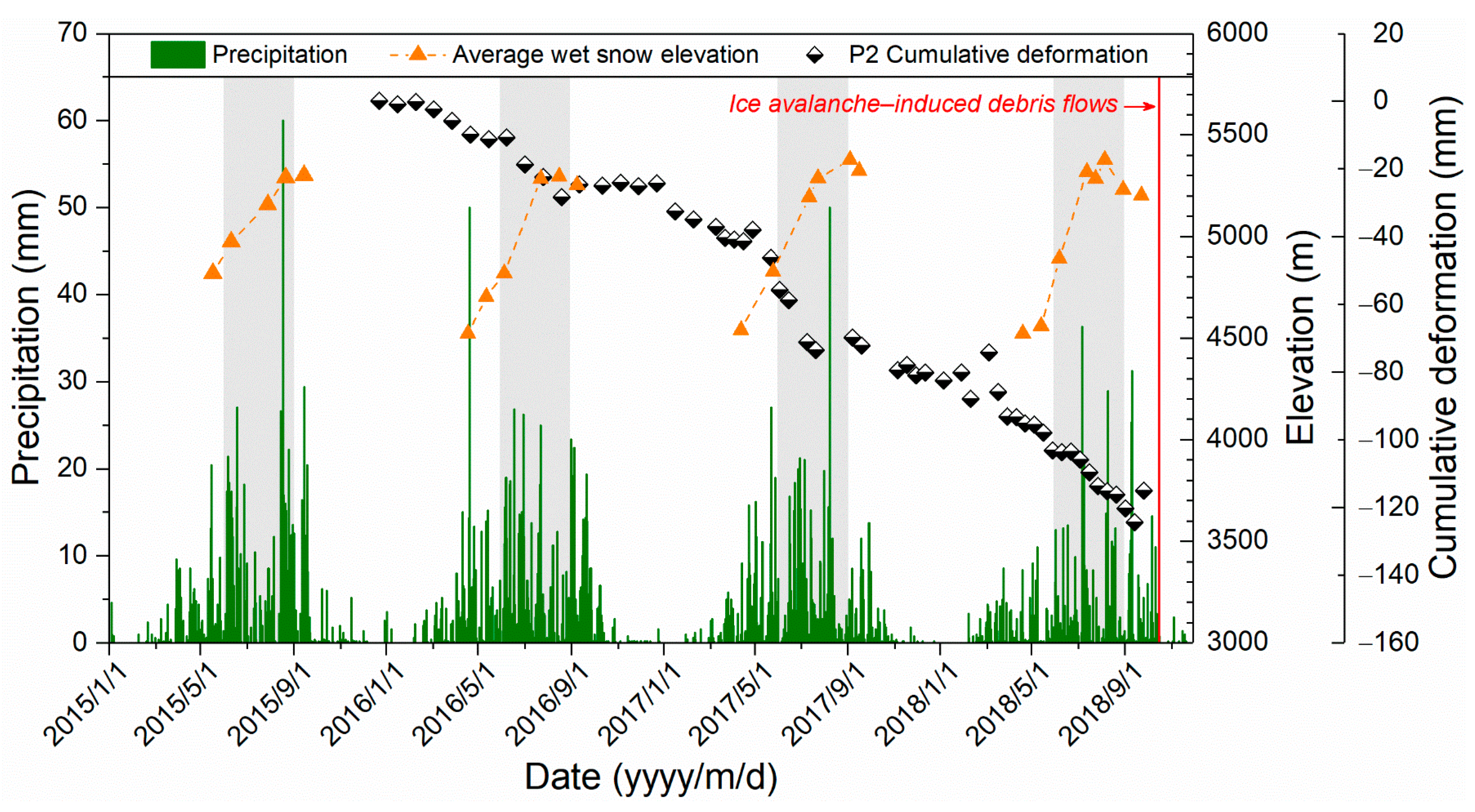
5.1. Deformation Measured Using InSAR and Snowmelt Changes
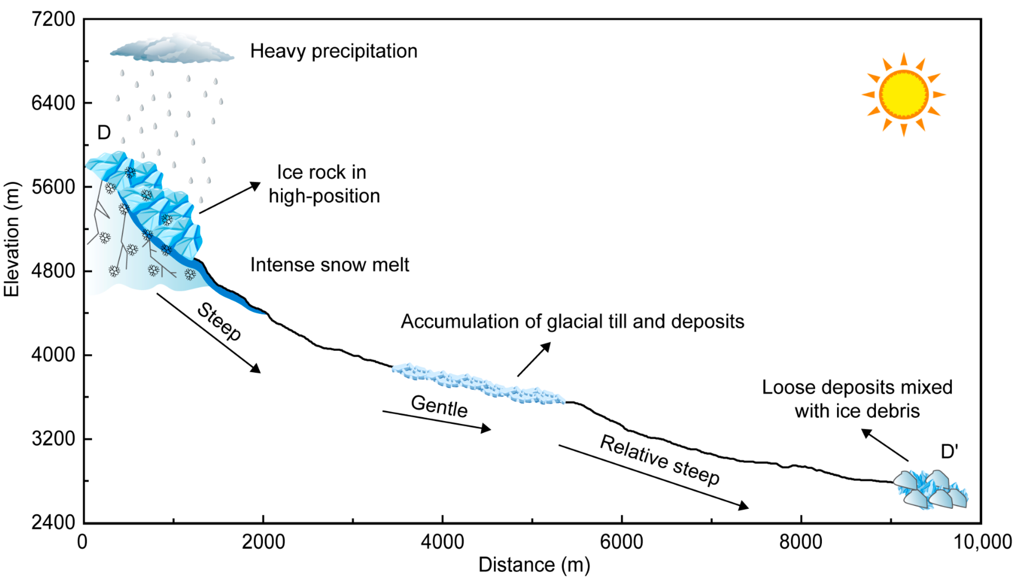
5.2. Seismic and Topographic Characteristics
6. Conclusions
Author Contributions
Funding
Data Availability Statement
Acknowledgments
Conflicts of Interest
References
- Immerzeel, W.W.; Lutz, A.; Andrade, M.; Bahl, A.; Biemans, H.; Bolch, T.; Hyde, S.; Brumby, S.; Davies, B.; Elmore, A. Importance and vulnerability of the world’s water towers. Nature 2020, 577, 364–369. [Google Scholar] [CrossRef] [PubMed]
- Yao, T.; Xue, Y.; Chen, D.; Chen, F.; Thompson, L.; Cui, P.; Koike, T.; Lau, W.K.-M.; Lettenmaier, D.; Mosbrugger, V. Recent third pole’s rapid warming accompanies cryospheric melt and water cycle intensification and interactions between monsoon and environment: Multidisciplinary approach with observations, modeling, and analysis. Bull. Am. Meteorol. Soc. 2019, 100, 423–444. [Google Scholar] [CrossRef]
- Miles, E.; McCarthy, M.; Dehecq, A.; Kneib, M.; Fugger, S.; Pellicciotti, F. Health and sustainability of glaciers in High Mountain Asia. Nat. Commun. 2021, 12, 2868. [Google Scholar] [CrossRef] [PubMed]
- Kirschbaum, D.; Watson, C.S.; Rounce, D.R.; Shugar, D.H.; Kargel, J.S.; Haritashya, U.K.; Amatya, P.; Shean, D.; Anderson, E.R.; Jo, M. The state of remote sensing capabilities of cascading hazards over High Mountain Asia. Front. Earth Sci. 2019, 7, 197. [Google Scholar] [CrossRef] [Green Version]
- Gao, J.; Yao, T.; Masson-Delmotte, V.; Steen-Larsen, H.C.; Wang, W. Collapsing glaciers threaten Asia’s water supplies. Nature 2019, 565, 19–21. [Google Scholar] [CrossRef] [Green Version]
- Kääb, A.; Leinss, S.; Gilbert, A.; Bühler, Y.; Gascoin, S.; Evans, S.G.; Bartelt, P.; Berthier, E.; Brun, F.; Chao, W.-A. Massive collapse of two glaciers in western Tibet in 2016 after surge-like instability. Nat. Geosci. 2018, 11, 114–120. [Google Scholar] [CrossRef] [Green Version]
- An, B.; Wang, W.; Yang, W.; Wu, G.; Guo, Y.; Zhu, H.; Gao, Y.; Bai, L.; Zhang, F.; Zeng, C. Process, mechanisms, and early warning of glacier collapse-induced river blocking disasters in the Yarlung Tsangpo Grand Canyon, southeastern Tibetan Plateau. Sci. Total Environ. 2021, 816, 151652. [Google Scholar] [CrossRef]
- Deng, M.; Chen, N.; Liu, M. Meteorological factors driving glacial till variation and the associated periglacial debris flows in Tianmo Valley, south-eastern Tibetan Plateau. Nat. Hazards Earth Syst. Sci. 2017, 17, 345–356. [Google Scholar] [CrossRef] [Green Version]
- Chen, C.; Zhang, L.; Xiao, T.; He, J. Barrier lake bursting and flood routing in the Yarlung Tsangpo Grand Canyon in October 2018. J. Hydrol. 2020, 583, 124603. [Google Scholar] [CrossRef]
- Anderson, R.S.; Anderson, L.S.; Armstrong, W.H.; Rossi, M.W.; Crump, S.E. Glaciation of alpine valleys: The glacier–debris-covered glacier–rock glacier continuum. Geomorphology 2018, 311, 127–142. [Google Scholar] [CrossRef]
- Faillettaz, J.; Funk, M.; Vincent, C. Avalanching glacier instabilities: Review on processes and early warning perspectives. Rev. Geophys. 2015, 53, 203–224. [Google Scholar] [CrossRef] [Green Version]
- Jacquemart, M.; Loso, M.; Leopold, M.; Welty, E.; Berthier, E.; Hansen, J.S.; Sykes, J.; Tiampo, K. What drives large-scale glacier detachments? Insights from Flat Creek glacier, St. Elias Mountains, Alaska. Geology 2020, 48, 703–707. [Google Scholar] [CrossRef]
- Li, W.; Zhao, B.; Xu, Q.; Scaringi, G.; Lu, H.; Huang, R. More frequent glacier-rock avalanches in Sedongpu gully are blocking the Yarlung Zangbo River in eastern Tibet. Landslides 2022, 19, 589–601. [Google Scholar] [CrossRef]
- Keefer, D.K. Investigating landslides caused by earthquakes–a historical review. Surv. Geophys. 2002, 23, 473–510. [Google Scholar] [CrossRef]
- Yang, L.; Zhao, C.; Lu, Z.; Yang, C.; Zhang, Q. Three-dimensional time series movement of the cuolangma glaciers, southern tibet with sentinel-1 imagery. Remote Sens. 2020, 12, 3466. [Google Scholar] [CrossRef]
- Yang, W.; Wang, Y.; Wang, Y.; Ma, C.; Ma, Y. Retrospective deformation of the Baige landslide using optical remote sensing images. Landslides 2020, 17, 659–668. [Google Scholar] [CrossRef]
- Piroton, V.; Schlögel, R.; Barbier, C.; Havenith, H.-B. Monitoring the recent activity of landslides in the Mailuu-Suu Valley (Kyrgyzstan) using radar and optical remote sensing techniques. Geosciences 2020, 10, 164. [Google Scholar] [CrossRef]
- Scaioni, M.; Longoni, L.; Melillo, V.; Papini, M. Remote sensing for landslide investigations: An overview of recent achievements and perspectives. Remote Sens. 2014, 6, 9600–9652. [Google Scholar] [CrossRef] [Green Version]
- Zhou, Y.; Li, Z.; Li, J.; Zhao, R.; Ding, X. Glacier mass balance in the Qinghai–Tibet Plateau and its surroundings from the mid-1970s to 2000 based on Hexagon KH-9 and SRTM DEMs. Remote Sens. Environ. 2018, 210, 96–112. [Google Scholar] [CrossRef]
- Ferretti, A.; Prati, C.; Rocca, F. Permanent scatterers in SAR interferometry. IEEE Trans. Geosci. Remote Sens. 2001, 39, 8–20. [Google Scholar] [CrossRef]
- Hooper, A. A multi-temporal InSAR method incorporating both persistent scatterer and small baseline approaches. Geophys. Res. Lett. 2008, 35, L16302–L16309. [Google Scholar] [CrossRef] [Green Version]
- Berardino, P.; Fornaro, G.; Lanari, R.; Sansosti, E. A New Algorithm for Surface Deformation Monitoring Based on Small Baseline Differential SAR Interferograms. IEEE Trans. Geosci. Remote Sens. 2002, 40, 2375–2383. [Google Scholar] [CrossRef] [Green Version]
- Carlà, T.; Intrieri, E.; Raspini, F.; Bardi, F.; Farina, P.; Ferretti, A.; Colombo, D.; Novali, F.; Casagli, N. Perspectives on the prediction of catastrophic slope failures from satellite InSAR. Sci. Rep. 2019, 9, 14137. [Google Scholar] [CrossRef] [PubMed] [Green Version]
- Dong, J.; Zhang, L.; Tang, M.; Liao, M.; Xu, Q.; Gong, J.; Ao, M. Mapping landslide surface displacements with time series SAR interferometry by combining persistent and distributed scatterers: A case study of Jiaju landslide in Danba, China. Remote Sens. Environ. 2018, 205, 180–198. [Google Scholar] [CrossRef]
- Zhao, C.; Lu, Z.; Zhang, Q.; de La Fuente, J. Large-area landslide detection and monitoring with ALOS/PALSAR imagery data over Northern California and Southern Oregon, USA. Remote Sens. Environ. 2012, 124, 348–359. [Google Scholar] [CrossRef]
- Dong, J.; Zhang, L.; Li, M.; Yu, Y.; Liao, M.; Gong, J.; Luo, H. Measuring precursory movements of the recent Xinmo landslide in Mao County, China with Sentinel-1 and ALOS-2 PALSAR-2 datasets. Landslides 2018, 15, 135–144. [Google Scholar] [CrossRef]
- Intrieri, E.; Raspini, F.; Fumagalli, A.; Lu, P.; Del Conte, S.; Farina, P.; Allievi, J.; Ferretti, A.; Casagli, N. The Maoxian landslide as seen from space: Detecting precursors of failure with Sentinel-1 data. Landslides 2018, 15, 123–133. [Google Scholar] [CrossRef] [Green Version]
- Kang, Y.; Lu, Z.; Zhao, C.; Zhang, Q.; Kim, J.-W.; Niu, Y. Diagnosis of Xinmo (China) landslide based on interferometric synthetic aperture radar observation and modeling. Remote Sens. 2019, 11, 1846. [Google Scholar] [CrossRef] [Green Version]
- Zhang, Y.; Meng, X.; Jordan, C.; Novellino, A.; Dijkstra, T.; Chen, G. Investigating slow-moving landslides in the Zhouqu region of China using InSAR time series. Landslides 2018, 15, 1299–1315. [Google Scholar] [CrossRef]
- Zhang, Y.; Meng, X.; Chen, G.; Qiao, L.; Zeng, R.; Chang, J. Detection of geohazards in the Bailong River Basin using synthetic aperture radar interferometry. Landslides 2016, 13, 1273–1284. [Google Scholar] [CrossRef]
- Dunning, S.A.; Rosser, N.J.; McColl, S.T.; Reznichenko, N.V. Rapid sequestration of rock avalanche deposits within glaciers. Nat. Commun. 2015, 6, 7964. [Google Scholar] [CrossRef] [PubMed] [Green Version]
- Karbou, F.; Veyssière, G.; Coleou, C.; Dufour, A.; Gouttevin, I.; Durand, P.; Gascoin, S.; Grizonnet, M. Monitoring Wet Snow Over an Alpine Region Using Sentinel-1 Observations. Remote Sens. 2021, 13, 381. [Google Scholar] [CrossRef]
- Ballesteros-Cánovas, J.A.; Trappmann, D.; Madrigal-González, J.; Eckert, N.; Stoffel, M. Climate warming enhances snow avalanche risk in the Western Himalayas. Proc. Natl. Acad. Sci. USA 2018, 115, 3410–3415. [Google Scholar] [CrossRef] [PubMed] [Green Version]
- Vergara Dal Pont, I.; Moreiras, S.M.; Santibanez Ossa, F.; Araneo, D.; Ferrando, F. Debris flows triggered from melt of seasonal snow and ice within the active layer in the semi-arid Andes. Permafr. Periglac. Process. 2020, 31, 57–68. [Google Scholar] [CrossRef]
- McGrath, D.; Webb, R.; Shean, D.; Bonnell, R.; Marshall, H.P.; Painter, T.H.; Molotch, N.P.; Elder, K.; Hiemstra, C.; Brucker, L. Spatially extensive ground-penetrating radar snow depth observations during NASA’s 2017 SnowEx campaign: Comparison with In situ, airborne, and satellite observations. Water Resour. Res. 2019, 55, 10026–10036. [Google Scholar] [CrossRef] [Green Version]
- Edemsky, D.; Popov, A.; Prokopovich, I.; Garbatsevich, V. Airborne Ground Penetrating Radar, Field Test. Remote Sens. 2021, 13, 667. [Google Scholar] [CrossRef]
- Nagler, T.; Rott, H. Retrieval of wet snow by means of multitemporal SAR data. IEEE Trans. Geosci. Remote Sens. 2000, 38, 754–765. [Google Scholar] [CrossRef]
- Huang, L.; Li, Z.; Tian, B.-S.; Chen, Q.; Liu, J.-L.; Zhang, R. Classification and snow line detection for glacial areas using the polarimetric SAR image. Remote Sens. Environ. 2011, 115, 1721–1732. [Google Scholar] [CrossRef]
- Nagler, T.; Rott, H.; Ripper, E.; Bippus, G.; Hetzenecker, M. Advancements for Snowmelt Monitoring by Means of Sentinel-1 SAR. Remote Sens. 2016, 8, 348. [Google Scholar] [CrossRef] [Green Version]
- Baghdadi, N.; Gauthier, Y.; Bernier, M. Capability of multitemporal ERS-1 SAR data for wet-snow mapping. Remote Sens. Environ. 1997, 60, 174–186. [Google Scholar] [CrossRef]
- Li, Z.; Li, B.; Gao, Y.; Wang, M.; Zhao, C.; Liu, X. Remote sensing interpretation of development characteristics of high-position geological hazards in Sedongpu gully, downstream of Yarlung Zangbo River. Chin. J. Geol. Hazard Control 2021, 32, 33–41. [Google Scholar] [CrossRef]
- Ding, Y.; Zhang, S.; Zhao, L.; Li, Z.; Kang, S. Global warming weakening the inherent stability of glaciers and permafrost. Sci. Bull. 2019, 64, 245–253. [Google Scholar] [CrossRef] [Green Version]
- Casu, F.; Manzo, M.; Lanari, R. A quantitative assessment of the SBAS algorithm performance for surface deformation retrieval from DInSAR data. Remote Sens. Environ. 2006, 102, 195–210. [Google Scholar] [CrossRef]
- Goldstein, R.M.; Werner, C.L. Radar interferogram filtering for geophysical applications. Geophys. Res. Lett. 1998, 25, 4035–4038. [Google Scholar] [CrossRef] [Green Version]
- Pepe, A.; Lanari, R. On the Extension of the Minimum Cost Flow Algorithm for Phase Unwrapping of Multitemporal Differential SAR Interferograms. IEEE Trans. Geoence Remote Sens. 2006, 44, 2374–2383. [Google Scholar] [CrossRef]
- Pepe, A.; Berardino, P.; Bonano, M.; Euillades, L.D.; Lanari, R.; Sansosti, E. SBAS-based satellite orbit correction for the generation of DInSAR time-series: Application to RADARSAT-1 data. IEEE Trans. Geosci. Remote Sens. 2011, 49, 5150–5165. [Google Scholar] [CrossRef]
- Wu, Q.; Jia, C.; Chen, S.; Li, H. SBAS-InSAR based deformation detection of urban land, created from mega-scale mountain excavating and valley filling in the Loess Plateau: The case study of Yan’an City. Remote Sens. 2019, 11, 1673. [Google Scholar] [CrossRef] [Green Version]
- Baghdadi, N.; Gauthier, Y.; Bernier, M.; Fortin, J.P. Potential and limitations of RADARSAT SAR data for wet snow monitoring. Geosci. Remote Sens. IEEE Trans. 2000, 38, 316–320. [Google Scholar] [CrossRef]
- Nagler, T.; Rott, H.; Malcher, P.; Müller, F. Assimilation of meteorological and remote sensing data for snowmelt runoff forecasting. Remote Sens. Environ. 2008, 112, 1408–1420. [Google Scholar] [CrossRef]
- Snehmania; Venkataraman, G.; Nigam, A.K.; Singh, G. Development of an inversion algorithm for dry snow density estimation and its application with ENVISAT-ASAR dual co-polarization data. Geocarto Int. 2010, 25, 597–616. [Google Scholar] [CrossRef]
- Fuhrmann, T.; Garthwaite, M.C. Resolving three-dimensional surface motion with InSAR: Constraints from multi-geometry data fusion. Remote Sens. 2019, 11, 241. [Google Scholar] [CrossRef] [Green Version]
- Guo, R.; Li, S.; Chen, Y.n.; Li, X.; Yuan, L. Identification and monitoring landslides in Longitudinal Range-Gorge Region with InSAR fusion integrated visibility analysis. Landslides 2021, 18, 551–568. [Google Scholar] [CrossRef]
- Zhao, B.; Li, W.; Wang, Y.; Lu, J.; Li, X. Landslides triggered by the Ms 6.9 Nyingchi earthquake, China (18 November 2017): Analysis of the spatial distribution and occurrence factors. Landslides 2019, 16, 765–776. [Google Scholar] [CrossRef]
- Snapir, B.; Momblanch, A.; Jain, S.; Waine, T.W.; Holman, I.P. A method for monthly mapping of wet and dry snow using Sentinel-1 and MODIS: Application to a Himalayan river basin. Int. J. Appl. Earth Obs. Geoinf. 2019, 74, 222–230. [Google Scholar] [CrossRef] [Green Version]
- Liu, C.; Chen, C. Achievements and countermeasures in risk reduction of geological disasters in China. J. Eng. Geol. 2020, 28, 375–383. [Google Scholar] [CrossRef]


| Data | Parameter | Description |
|---|---|---|
| Sentinel-1A/B | Orbit direction | Descending/Ascending |
| Product type | SLC | |
| Polarization mode | VV | |
| Radar wavelength | 5.6 cm | |
| Acquisition mode | IW | |
| Pixel spacing (azimuth × range) | 13.96 m × 2.32 m | |
| Acquisition period | 29 October 2014–13 October 2018 | |
| ASTER GDEM | Resolution | 30 m |
| Number | Average Deformation (mm/Year) | Maximum Deformation (mm/Year) | Maximum Cumulative Displacement (mm) | Slide |
|---|---|---|---|---|
| P1 | −30.90 | −32.52 | −76.05 | Yes |
| P2 | −45.21 | −48.52 | −120.72 | Yes |
| P3 | −40.28 | −44.39 | −97.69 | No |
| P4 | −34.93 | −37.05 | −112.46 | No |
| P5 | −35.04 | −40.46 | −101.32 | No |
| P6 | −34.64 | −37.73 | −93.86 | No |
| P7 | −28.76 | −31.14 | −79.79 | No |
| P8 | −48.44 | −51.99 | −137.52 | Yes |
| Date | Wet Snow Area (km2) | Date | Wet Snow Area (km2) |
|---|---|---|---|
| 14 May 2015–21 May 2015 | 8.9572 | 9 July 2017–14 July 2017 | 7.1532 |
| 7 June 2015–14 June 2015 | 5.2452 | 21 July 2017–26 July 2017 | 6.7004 |
| 25 July 2015–1 August 2015 | 3.672 | 31 August 2017–7 September2017 | 4.8912 |
| 18 August 2015–25 August 2015 | 4.4884 | 12 September 2017–19 September 2017 | 5.0164 |
| 11 September 2015–18 September 2015 | 4.7032 | 16 April 2018–23 April 2018 | 5.728 |
| 14 April 2016–21 April 2016 | 9.6672 | 10 May 2018–17 May 2018 | 7.4168 |
| 8 May 2016–15 May 2016 | 13.5672 | 3 June 2018–10 June 2018 | 9.852 |
| 1 June 2016–8 June 2016 | 10.988 | 9 July 2018–16 July 2018 | 5.0184 |
| 19 July 2016–26 July 2016 | 6.3444 | 21 July 2018–28 July 2018 | 5.4304 |
| 12 August 2016–19 August 2016 | 5.9448 | 2 August 2018–9 August 2018 | 5.1408 |
| 5 September 2016–12 September 2016 | 6.5332 | 26 August 2018–2 September 2018 | 5.1996 |
| 9 April 2017–16 April 2017 | 7.09 | 19 September 2018–26 September 2018 | 6.3752 |
| 22 May 2017–27 May 2017 | 12.4956 |
Publisher’s Note: MDPI stays neutral with regard to jurisdictional claims in published maps and institutional affiliations. |
© 2022 by the authors. Licensee MDPI, Basel, Switzerland. This article is an open access article distributed under the terms and conditions of the Creative Commons Attribution (CC BY) license (https://creativecommons.org/licenses/by/4.0/).
Share and Cite
Luo, S.; Xiong, J.; Liu, S.; Hu, K.; Cheng, W.; Liu, J.; He, Y.; Sun, H.; Cui, X.; Wang, X. New Insights into Ice Avalanche-Induced Debris Flows in Southeastern Tibet Using SAR Technology. Remote Sens. 2022, 14, 2603. https://doi.org/10.3390/rs14112603
Luo S, Xiong J, Liu S, Hu K, Cheng W, Liu J, He Y, Sun H, Cui X, Wang X. New Insights into Ice Avalanche-Induced Debris Flows in Southeastern Tibet Using SAR Technology. Remote Sensing. 2022; 14(11):2603. https://doi.org/10.3390/rs14112603
Chicago/Turabian StyleLuo, Siyuan, Junnan Xiong, Shuang Liu, Kaiheng Hu, Weiming Cheng, Jun Liu, Yufeng He, Huaizhang Sun, Xingjie Cui, and Xin Wang. 2022. "New Insights into Ice Avalanche-Induced Debris Flows in Southeastern Tibet Using SAR Technology" Remote Sensing 14, no. 11: 2603. https://doi.org/10.3390/rs14112603
APA StyleLuo, S., Xiong, J., Liu, S., Hu, K., Cheng, W., Liu, J., He, Y., Sun, H., Cui, X., & Wang, X. (2022). New Insights into Ice Avalanche-Induced Debris Flows in Southeastern Tibet Using SAR Technology. Remote Sensing, 14(11), 2603. https://doi.org/10.3390/rs14112603