An Integrated Algorithm for Extracting Terrain Feature-Point Clusters Based on DEM Data

Abstract

Terrain feature points, such as the peaks and saddles, are the basic framework of surface topography and its undulations, which significantly affect the spatial distribution of surface topography. In the past, terrain feature points were extracted separately for each type, while the internal connections between the terrain feature points were ignored. Therefore, this work proposes an integrated algorithm for extracting terrain feature-point clusters, including the peaks, saddles and runoff nodes, based on the DEM data. This method includes two main processes: positive terrain-constrained ridgeline extraction and terrain feature-point cluster extraction. Firstly, a threshold determination method of flow accumulation in the hydrological analysis is proposed by combining morphological characteristics with runoff simulation, and the ridgelines are extracted based on this threshold. Subsequently, the peaks and their control areas are extracted by space segmentation. Meanwhile, the saddles and runoff nodes are obtained by spatial intersection. Finally, the integrated terrain feature-point clusters are obtained by merging the three extracted terrain feature points. This method was experimented with in the six typical sample areas in Shaanxi Province and verified its results by contour lines and optical images. It shows that the spatial positions of the extracted terrain feature clusters are accurate, and the coupling relationships are great. Finally, the experiments show that the statistical attributes of point clusters and their spatial distribution trends have an obvious correlation with geomorphic types and geomorphic zoning, which can provide an important reference for geomorphic zoning and mapping.

1. Introduction

The terrain surface is composed of a series of characteristic elements (including point, line and surface elements), and its morphology and combination characteristics can be used as the symbolic carrier of the interactions among the earth’s internal tectonic movements, surface processes and climate evolution [1,2,3]. Among them, terrain feature-point clusters, including mountain peaks, saddles and runoff nodes, are widely distributed on the terrain surface, which are the controlling links in describing the terrain’s morphological structure and formation. These three kinds of terrain feature points can not only describe an aspect of terrain independently, but also have good coupling, matching quantity and topological connection relationships among them, which can be combined to describe terrain relief, distribution difference, dynamic development and change characteristics as a whole [4]. Thus, this paper proposes terrain feature-point clusters, which are organic structures with distance, orientation and topological constraints consisting of peaks distributed along the ridgelines and their control ranges, related saddles and runoff nodes. As a high-level abstraction of natural terrain, the terrain feature-point cluster links the micro-analysis and macro-analysis of terrain, which presents the advantages of loading multi-level information. For example, the connections between peaks and saddles describe the undulation degree of ridge and fragmentation characteristics in the region, and the connections between saddles and runoff nodes describe the current topographic erosion characteristics and confluence kinetic energy characteristics. Meanwhile, topographic characteristics and spatial orientation characteristics reflect the topographic differences between different geomorphic regions, which are the powerful tools for geomorphological regionalization.

Existing studies usually focus on a single terrain feature point [5,6,7,8]. Due to the lack of considering the matching and coupling of these points from the overall and global perspective, there are many mismatches in the spatial connection relations and other aspects among different types of point cluster elements obtained by existing methods [9]. Chen and Guevara proposed the very important points (VIP), which are important for displaying terrain surface, and implemented the VIP extraction based on digital elevation model (DEM) data [10]. On this basis, Gökgöz and Hacar proposed important points and edges (IPE) and their extraction method [11]. However, all of these methods focus on the TIN (Triangulated Irregular Network)’s construction, which only considers the points’ importance to the terrain surface, ignoring the geomorphological significance of points and their intrinsic relations. Morse developed Cayley and Maxwell’s topographic models [12,13] based on the differential topology, and applied his theory to geodesics and other critical point extraction in high-dimensional manifolds [14,15]. Discrete Morse theory and methods were developed to extract critical points from discrete data (e.g., DEM and high-dimensional images) [16,17]. At the same time, surface models such as Reed graph [18] and Pfaltz’s graph [19] were used to organize these critical points and lines. These methods can obtain terrain feature points and lines containing topological information, providing a new idea in feature extraction and terrain representation. However, these methods focus on the gradient of manifolds from a topological perspective and lack consideration of the geomorphological significance and scale dependence [20,21]. Therefore, it is urgent to build an integrated terrain feature-point cluster extraction method that can realize the simultaneous extraction of terrain feature-point clusters to ensure the accuracy of point cluster positions and the relative consistency within the clusters.

Although the peaks exist as point elements, they are essentially abstractions of the individual mountain in geographic space, occupying the corresponding spatial area, and the saddles are located at the intersections of the control areas’ boundaries corresponding to these peaks. If the original terrain is divided, the control areas of each peak can be obtained, and the saddles can be obtained by intersecting the control area boundaries with the ridgelines. From the saddles, the peaks can be connected along the watershed lines, and along the ravine lines are runoff nodes. In fact, the peaks’ control areas and the watershed areas can be seen as the unstable Morse complex and stable Morse complex in the Morse theory, respectively. Meanwhile, the saddles can be seen as the Morse–Smale complex [22]. The principle is shown in Figure 1.

Then the problem becomes how to extract ridgelines and the control areas of the peak accurately. Ridgelines are a definite and objective terrain feature object as one of the typical terrain structure lines. The current research on terrain structure line extraction mainly includes the section extreme value method [23,24], skeletonization method [2,25] and runoff simulation method [26,27,28]. The terrain profile analysis method includes three major steps: candidate point extraction, pseudo candidate point elimination, and structure line construction, but the analysis process generally only considers specific directions and ignores other directions. The skeletonization method assumes that the terrain structure lines are symmetrically distributed to the left and right, which is obviously inconsistent with the fact. Currently, the runoff simulation method is widely used to extract the terrain structure lines, among which the deterministic eight-node (D8) algorithm [26,29] is most commonly used. However, due to the lack of an explicit threshold selection instruction in the runoff simulation, the uncertainty of the threshold in this process makes the extracted terrain structure lines poorly comparable [30,31,32]. As for the peak control area acquisition, Luo et al. proposed the space segmentation method with the height difference limitation [33]. The original terrain was turned into an anti-terrain, and a threshold-limited filling process was performed. Then, the anti-terrain watershed areas [34,35,36,37] were extracted as the mountain control areas. This method draws on the hydrological viewpoint, and the obtained mountain control areas are consistent with geomorphological perception.

This paper proposes an integrated method for extracting terrain feature-point clusters to overcome the above limitations. Firstly, the ridgelines are extracted by combining the morphological features with the runoff simulation method. Meanwhile, the peaks and their control areas are extracted by the spatial subdivision method [33]. Then, the ridgelines intersect with the peaks’ control area boundaries to obtain the saddles, and the control area boundaries are self-intersected to obtain the runoff nodes. Finally, the integrated terrain feature-point clusters are obtained by merging these extracted point clusters.

The main contributions of our work are as follows: (1) an integrated method for extracting terrain feature-point clusters is proposed, revealing the structure and intrinsic relationship of the feature points; (2) a way for determining the flow accumulation threshold for ridgeline extraction based on the runoff simulation method is put forward, representing an important attempt at digital terrain analysis; (3) the saddle dissection index is proposed and the geomorphological significance of point clusters is explored.

Section 2 elaborates the materials and methods of this study, including the study area and data (Section 2.1), positive terrain-constrained ridgeline extraction method (Section 2.2.1), and terrain feature-point cluster extraction method (Section 2.2.2). Section 3 introduces and validates the experiment results and discusses their geomorphology significance, including the results of optimal threshold determination (Section 3.1), extraction results and validations of point clusters (Section 3.2), statistics of point clusters’ properties (Section 3.3), and point clusters’ properties and geomorphological regionalization (Section 3.4).

2. Materials and Methods

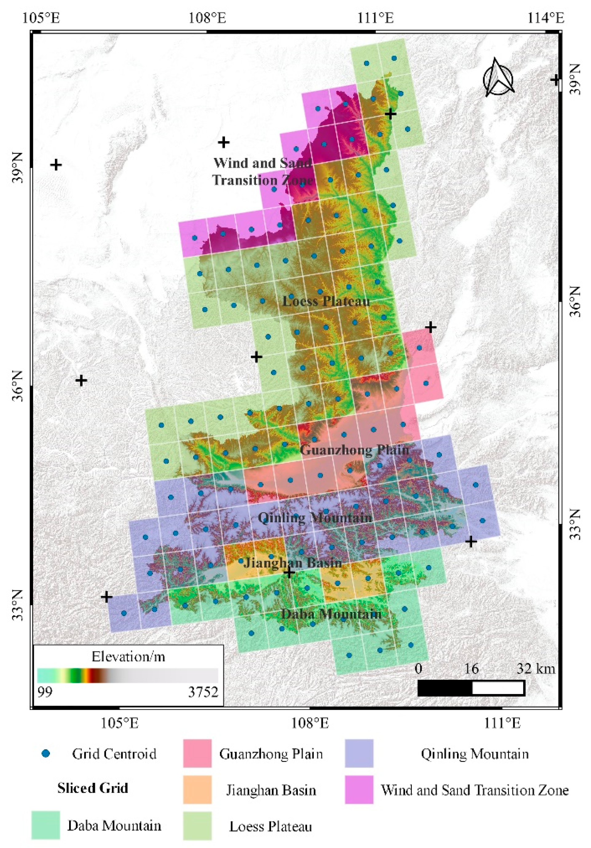
2.1. Study Area and Data

The study area is Shaanxi Province (105°29′E to 111°15′E, 31°42′N to 39°35′N), which is located in the hinterland of northwest China, with a land area of 205,700 km². The northern mountains and the Qinling Mountains divide Shaanxi Province into three natural regions: the northern part is the northern Shaanxi plateau, including the wind–sand landscape and the Loess Plateau (including loess tablelands, hills and ridges), with sparse precipitation and serious soil erosion; the central part is the Guanzhong Plain, which is high in the west and low in the east, and is the urban agglomeration in the province with strong human activities; and the southern part is the Qinba Mountains, which has the landform structure of “two mountains sandwiching one river”, and there are serious natural hazards such as landslides and flash flooding. The various geomorphic differentiation causes the spatial heterogeneity of natural disasters and human disturbances, providing a case basis for the study of terrain point clusters and geomorphic differentiation (Figure 2a).

In the selection of experimental sample areas, considering various factors such as the representativeness of the experimental sample areas, the richness of landform types and the existing research bases, the six counties of Hanyin (HT), Mizhi (MZ), Ningshan (NS), Yanchuan (YC), Zhen’an (ZA) and Zhenba (ZB) were selected as typical sample areas in this study. These six sample areas represent different periods of loess landform evolution to a certain extent and cover the main landform types in Shaanxi Province [38]. The overview of these typical sample areas is shown in

Table 1. Overview of the typical sample areas.

Sample Area Name	Landform Type	Geomorphological Region
Ningshan County	Qinling middle and high mountains	Qinling Mountains
Zhen’an County	Qinling middle mountains	Qinling Mountains
Zhenba County	Daba middle mountains	Daba Mountains
Hanyin County	Low hills and mountains	Hanzhong low hill and basin area
Yanchuan County	Loess ridge	Loess Plateau
Mizhi County	Loess hill	Loess Plateau

and Figure 2b.

In this study, the DEM data are Shuttle Radar Topography Mission (SRTM) DEM, which were jointly measured by the National Aeronautics and Space Administration (NASA) and the US National Geospatial-Intelligence Agency (NGA), and covered almost 80% of the land surface area (from 60 N to 60 S). This time, we use the SRTM1 V3 downloaded from the United States Geological Survey (USGS) as the experimental data. The spatial resolution of these data is one arcsecond (30 m along the equator) with a nominal planimetric accuracy of ±20 m and an elevation accuracy of ±16 m, and the WGS84 coordinate system and EGM96 elevation datum (orthometric) are adopted. The study area and DEM data are shown in Figure 2.

2.2. Methods

The proposed method consists of two processes: positive terrain-constrained ridgeline extraction and terrain feature-point cluster extraction. According to this workflow, the digital elevation model data are used as input data to obtain the optimal flow accumulation threshold for ridgeline extraction based on morphological analysis, and ridgelines are extracted based on this optimal threshold. The peaks and their control areas are extracted using the spatial subdivision method [33], and the saddles and runoff nodes are obtained by spatial intersection. Finally, the integrated terrain feature-point clusters are obtained by merging these extracted point clusters.

Among them, the positive terrain-constrained ridgeline extraction includes three steps: (1) optimal window size determination of the positive terrain analysis; (2) optimal threshold determination of the flow accumulation; and (3) ridgeline extraction based on the runoff simulation method. In contrast, the terrain feature-point cluster extraction includes two main processes: peak extraction based on the spatial subdivision method and feature-point cluster extraction and calibration. More details of these steps are described in the following subsections.

2.2.1. Positive Terrain-Constrained Ridgeline Extraction

A positive terrain-constrained ridgeline extraction method is proposed to overcome the problem that it is difficult to determine the threshold of flow accumulation when extracting ridgelines using the traditional runoff simulation method. Combining morphological characteristics with runoff simulation, the simulated ridgelines are extracted using positive terrain membership degree and morphological analysis, and the optimal threshold of the flow accumulation is determined by the simulated ridgelines’ length. Then, the ridgelines are extracted using the runoff simulation method with the optimal flow accumulation threshold. The workflow of this method is shown in Figure 3.

Optimal window size determination of the positive terrain analysis. Ridgelines are the prominent structural line of positive terrain. Positive and negative terrain are relatively high or low parts of a certain area, respectively [39]. Based on the summary of previous studies, Zhou et al. concluded that the positive terrain of the loess ridges and hills area could be distinguished according to the valley lines, while other topography needs to be analyzed according to local terrain [40]. According to the above views, the positive terrain based on the DEM data can be defined as the relatively convex part under local window analysis, while the negative terrain can be defined as the relatively concave part. This can be distinguished by the macroscopic slope factor [41]:

$$P=H_{i,j}-({\displaystyle \sum _{k=1}^n{H}_k})/n$$

(1)

where H_i,j is the elevation value of the window’s center pixel, ${\displaystyle \sum _{k=1}^n{H}_k}$ is the sum of the elevation values in the window and n is the number of pixels in the window. When P > 0, the center pixel of the window is a positive terrain pixel. The multi-scale characteristic is ubiquitous in almost all geography-related fields [42,43]. Therefore, combined with Equation (1), it can be seen that the analysis window size plays a vital role in whether it is positive terrain. At present, the determination of the optimal analysis window size is mainly to seek the analysis window size. The local mean variance (LMV) method is simple to calculate and the results are easy to analyze, so it is widely used in scale analysis [44,45]. For regions with complex topography, such as karst areas, Li et al. proposed the local normalized variance [46]:

$$LNV=\frac{LMV}{r^2}$$

(2)

where LMV is the mean variance of the elevations in the analysis window, and r is the number of grid cells corresponding to the analysis window’s radius. The variance values are normalized to a uniform unit on one grid cell by dividing by the analysis window’s radius, which improves the comparability of the method across different regions. Since the topography of the Loess Plateau is more complex compared with that of the karst region, normalization using r² is not conducive to the presentation and analysis of topographic details. Therefore, based on the characteristics of the Loess Plateau, this paper derives the Loess local normalized variance:

$$LLNV=\frac{LMV}{2r}$$

(3)

Based on Equation (3), calculating the LLNV sequences:

$$\mathit{S}=\left\{LLN{V}_{k\times k}\right|\hspace{0.33em}k=3,s,\dots ,k-s,k\}$$

(4)

until it is found that:

$$LLN{V}_{k,k}-LLN{V}_{k-s,k-s}\le 0$$

(5)

This means looking for the local maximum point $LLN{V}_{k,k}$ of the LLNV sequence S, and its corresponding analysis window size k is the optimal analysis window size for positive terrain, where s is the step for finding the optimal analysis window size.

Optimal threshold determination of theflow accumulation. In hydrological analysis, the threshold of the flow accumulation significantly impacts the results. An optimal threshold of flow accumulation can greatly improve the quality of ridgelines obtained from the hydrological analysis. The ridgelines can be regarded as the skeleton lines of the positive terrain. Thus, the skeleton lines of positive terrain are obtained by thinning the positive terrain’s profile. Next, the ridgelines’ lengths extracted by the hydrological analysis are constrained by the skeleton lines’ lengths of the positive terrain, and thus, the optimal threshold of the flow accumulation in the hydrologic analysis is obtained by these constraints. Meanwhile, considering the boundary fuzziness and hierarchical separability of the terrain, it can be considered that there is a fuzziness about whether the center pixel in the window on the DEM data is positive terrain. Thus, positive terrain should be continuous in a sequence of multi-neighborhood analysis windows [47,48]. On the other hand, the hierarchical separability of terrain indicates that the multi-neighborhood analysis window must have the designated boundary of terrain hierarchy, and the terrain analysis from one terrain hierarchy to another has no transverse comparability [49]. Therefore, instead of directly using the positive terrain obtained with the optimal window size to extract the skeleton lines of the positive terrain, this paper introduces multiple neighborhoods to transform the positive terrain’s profile extraction into a fuzzy logic discrimination problem. On this basis, the membership degree of positive terrain is defined as:

$$\mathit{\lambda }={\displaystyle \sum _{k=min}^{max}H}{(i,j)}_k/(max-min+1)$$

(6)

where H(i, j)_k is the positive terrain state value corresponding to the pixel (i, j), if the pixel is in positive terrain when the window size is k, the state value is assigned to 1, otherwise it is 0; min and max are the minima and maxima side lengths of the analysis window, respectively. The min is usually set to 3, and the max is set to the optimal analysis window size obtained by the LLNV mentioned in Step 1. In Equation (6), the positive terrain obtained from neighborhood analysis with different windows sizes is considered to be of equal importance, and its weighting function is defined as equal weight. After obtaining the membership degree of positive terrain, the corresponding positive terrain outlines are acquired according to the corresponding membership degree requirements. Then, the skeleton lines of the positive terrain are obtained using a morphological thinning operation [50], and their lengths L are calculated. On the other hand, the watershed boundary lines under different flow accumulation thresholds are extracted using the runoff simulation method [29]. Next, the boundary lines obtained by each flow accumulation threshold T are filtered by positive terrain to obtain the potential ridgelines and calculate their lengths f(T), respectively. The flow accumulation threshold T for obtaining potential ridgelines can be constrained by the skeleton lines’ lengths L of the positive terrain extracted by morphological analysis. Finally, the best flow accumulation threshold $T’$ can be obtained by making L = f (T).

Ridgeline extraction based on the runoff simulation method. On natural surfaces, water always flows from high to low along the steepest direction and continuously converges downstream. The runoff simulation method determines the flow directions based on this view. The water volume is redistributed by the flow directions, and each cell’s final accumulated water volume in the DEM data after the end of the flow is calculated. Then, the cells whose sink volume is greater than the manual threshold are taken as sink points (valley points). Finally, these candidate points are connected according to specific rules, and the results are considered as the sink lines (valley line) [26,51]. The upstream supply areas can be obtained by searching upstream along the sink lines, and the watershed boundaries can be obtained by sketching the water supply areas. In this paper, the watershed boundaries are extracted using this method with the above best flow accumulation threshold $T’$. Eventually, the ridgelines corresponding to the positive terrain are obtained by filtering the watershed boundaries with positive terrain.

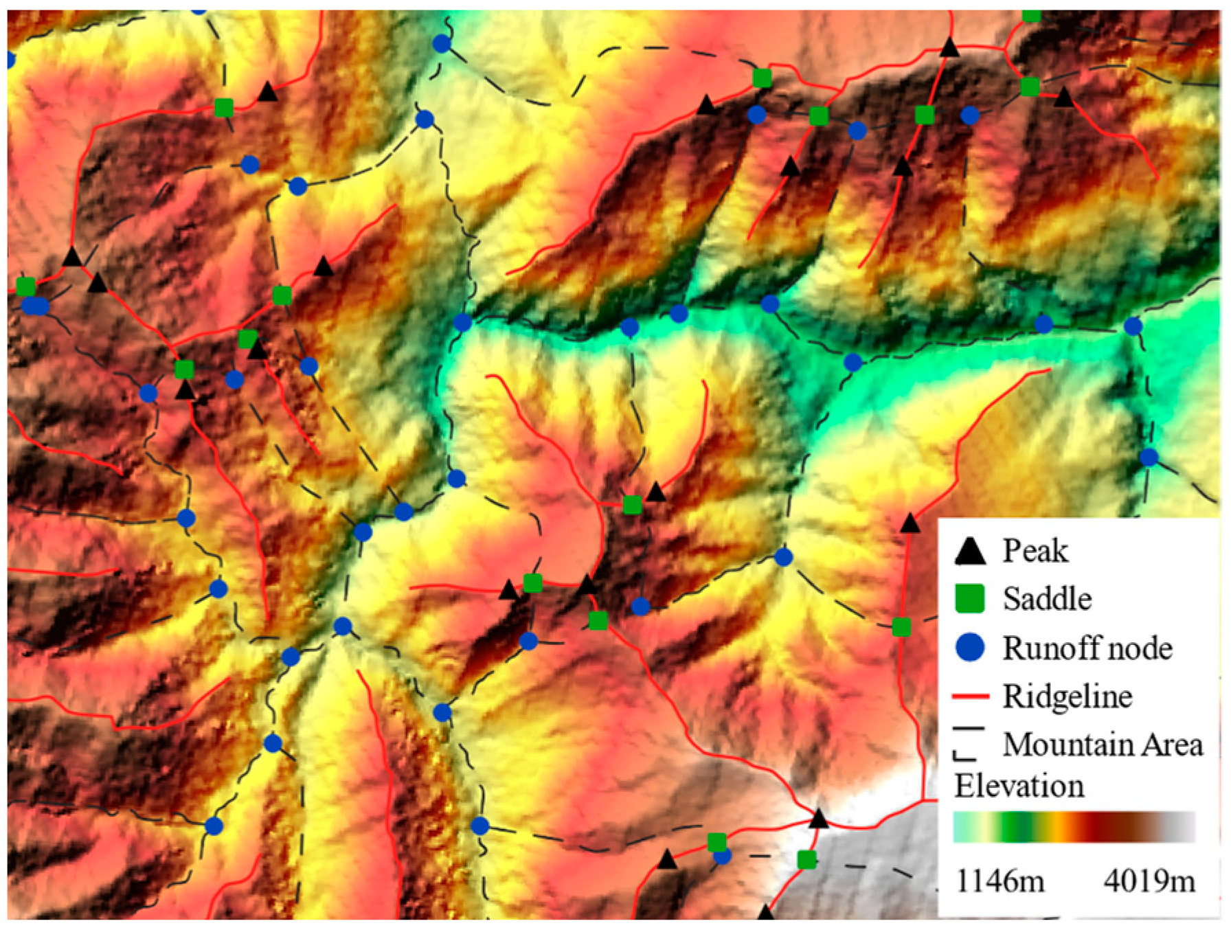
2.2.2. Terrain Feature-Point Cluster Extraction

Terrain feature points such as peaks, saddles and runoff nodes are the basic frameworks that constitute the surface topography and undulation changes. The candidate peaks and their control areas are obtained by the runoff simulation method. Then, the ridgelines are intersected with the boundaries of the peaks’ control area to obtain the candidate saddles. Meanwhile, the candidate runoff nodes are extracted by self-intersecting the peak control areas’ boundaries. Finally, the integrated terrain feature-point clusters are obtained by filtering and merging these feature points. The workflow of the proposed method is shown in Figure 4, including two steps: peak extraction by space segmentation and feature-point cluster extraction and verification.

Peaks extraction by space segmentation. The hydrological view believes that each watershed has its own control area, and there are multiple levels of sub-watersheds within this watershed. The watershed and its sub-watersheds at all levels are affected by specific topography, geomorphology, and lithology, showing a typical and irregular pattern. Correspondingly, the mountainous area can be considered as a positive geomorphic system consisting of the individual mountain, which controls different regional patches, respectively. Therefore, the original positive geomorphic mountains can be reversed to a negative watershed system, and the corresponding peaks can evolve into sinks in each watershed (Figure 5). Based on this viewpoint, the space segmentation method [33] is adopted to extract the peaks and their control areas. The original terrain is reversed into an anti-terrain. The anti-terrain is sink-filled under the Height Difference between Peaks and Saddles (HDPS) threshold limit, and the flow direction is calculated based on the sink-filled anti-terrain. Then, the peaks and their control area’s boundaries can be obtained by the anti-terrain watersheds extracted from the sink-filled flow direction. Among them, the sink filling’s threshold can be regarded as the peak control area’s height difference limit. The processes of this method are as follows: (1) calculate the anti-terrain, let $InvertDEM=DEM\times (-1)$; (2) fill sink on the anti-terrain with the given HDPS threshold; (3) calculate the flow direction of the filled anti-terrain; (4) extract sinks based on the filled anti-terrain flow direction as the candidate peaks of the original terrain; (5) extract the watershed of anti-terrain based on the flow direction and sinks of anti-terrain, as peak’s control area of the original terrain; and (6) obtain the peaks by searching the maximum elevation value of the original DEM in each peak’s control area. The needed peaks and their control areas are finally obtained through the above processes. It is worth noting that the “watershed extract” here is performed on the anti-terrain data, and its results are the candidate peaks’ control areas. Therefore, this step’s input data and output results are different from the “watershed extraction” in the step 3 of Section 2.2.1.

Feature-point cluster extraction and verification. The feature-point clusters include peaks, saddles, and runoff nodes, among which peaks are obtained by the space segmentation method described above. The saddles and runoff nodes are obtained by intersecting the ridgelines with the peak control areas’ boundary and self-intersecting the peak control areas, respectively. The point cluster verification is realized by positive and negative terrain filtering. According to the geomorphological viewpoint, the peaks and saddles are the convex points of the local terrain, which should be located in the positive terrain. Correspondingly, the runoff nodes should be located in the negative terrain. Therefore, the pseudo peaks and saddles can be eliminated by positive terrain checking, and pseudo runoff nodes can be eliminated by negative terrain checking. Finally, the integrated terrain feature-point clusters are obtained.

3. Results and Discussion

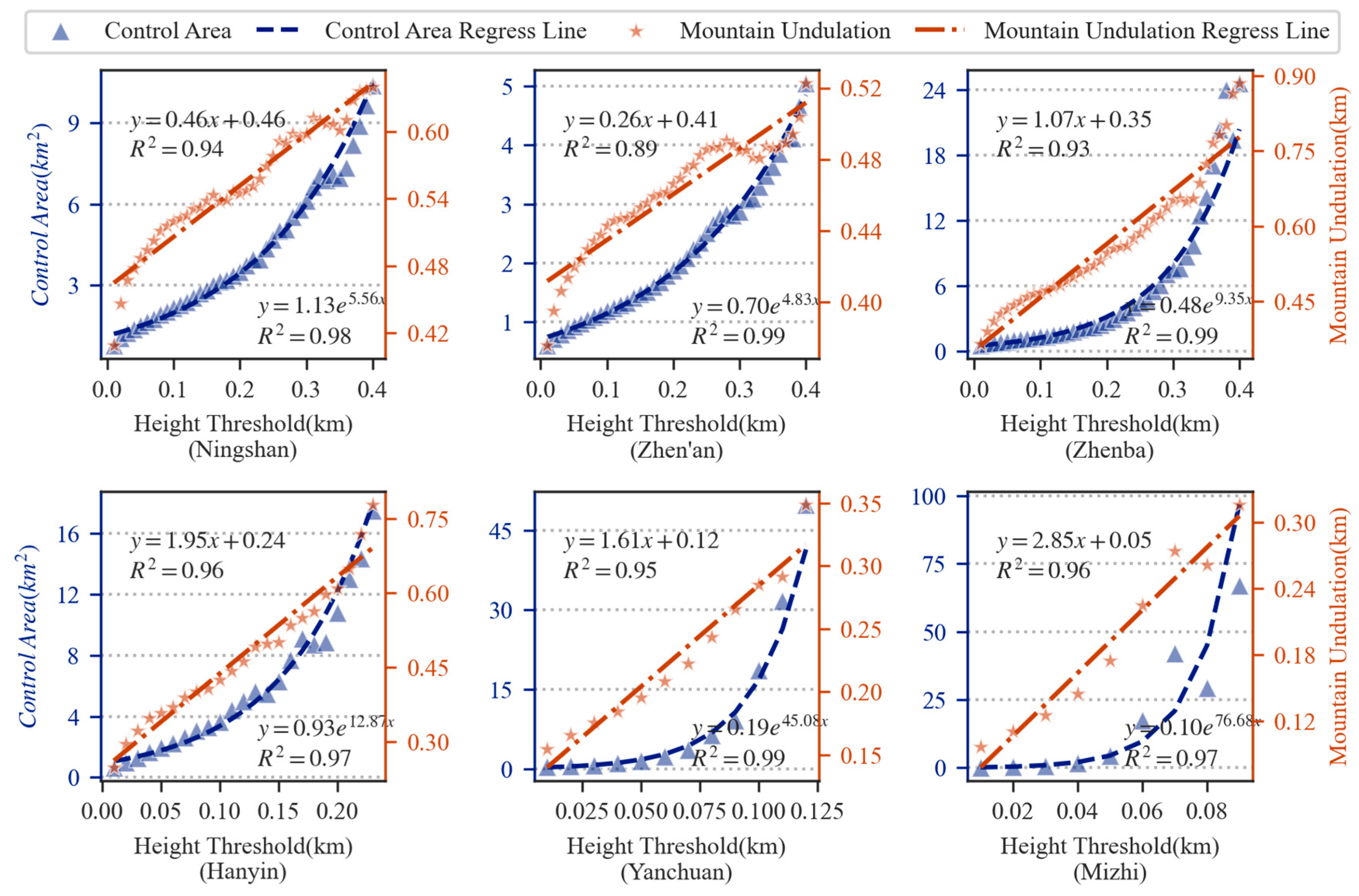
3.1. Results of Optimal Threshold Determination

As described in Section 2.2.1 of this paper, the LLNV and positive terrain constrain method were used to determine the optimal window size of the positive terrain analysis and the optimal threshold of flow accumulation in the runoff simulation, taking the six typical sample areas as an example. Then, the LLNVs and potential ridgeline lengths extracted using different parameters were counted, and their relationships are shown using a scatter plot in Figure 6. In Figure 6, the orange stars represent the relationships between the thresholds of flow accumulation in the runoff simulation and the extracted potential ridgelines’ lengths. It can be seen that there is a significant exponential relationship between the thresholds of flow accumulation and the potential ridgelines’ lengths, and the potential ridgeline length decreases with the increase of the flow accumulation’s threshold. The average value of the logistic regression’s coefficient of determination (R²) scores for the six typical sample areas reached 0.96, especially in the Yanchuan and Mizhi counties, where the R² scores reached 0.99 and 1.00, respectively. Therefore, it can be seen that an appropriate threshold of flow accumulation is of great significance for the potential ridgeline extraction. The blue triangles in Figure 6 represent the relationships between the window sizes of the positive terrain analysis and the corresponding LLNVs. It can be seen that there is a significant correlation between the window sizes and the LLNVs, and the LLNVs showed a trend of increasing first and then decreasing with the increase of the positive terrain analysis’s window size. The median value of the quadratic polynomial regression’s R² scores of the quadratic regression for the six typical sample areas reached 0.675. The optimal window sizes of the positive terrain analysis obtained by the proposed method are plotted as blue vertical dashed lines, all located at the extreme value points of the LLNV and adjacent to the fitted curve’s symmetry axis. It is noteworthy that the regression’s R² scores for Yanchuan and Mizhi counties show significantly higher values, which may be related to the sample area’s topographic relief and topographic complexity. To further analyze the relationship between the window size of the positive terrain analysis and the positive terrain, Ningxia County is taken as an example to show the positive terrain’s distribution with the window size from 3 × 3 to 51 × 51 (Figure 7), where Figure 7c shows the distribution of the positive terrain with the optimal analysis window (s = 21) sought by the proposed method. When the analysis window size is small (Figure 7a,b), the positive terrain’s distribution is more fragmented, and the flatlands are marked as positive terrain dispersedly, while there are still many positive terrain areas missing from the ridges. With the gradual increase of the analysis window size (Figure 7c–f), the positive terrain is mostly located on the ridges and highlands with a dendritic distribution. Meanwhile, the distribution of positive terrain tends to be stable, and the distribution does not change much with the increase of the window size starting from Figure 7c. Thus, the window size of the positive terrain analysis significantly impacts the distribution of the positive terrain, and the proposed method can obtain a typical analysis window size. To sum up, the proposed method for determining the optimal threshold of the flow accumulation and the window size of the positive terrain analysis has met the expectations.

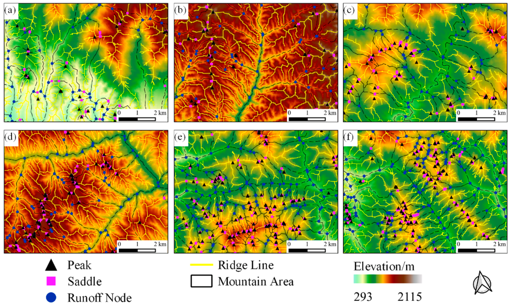
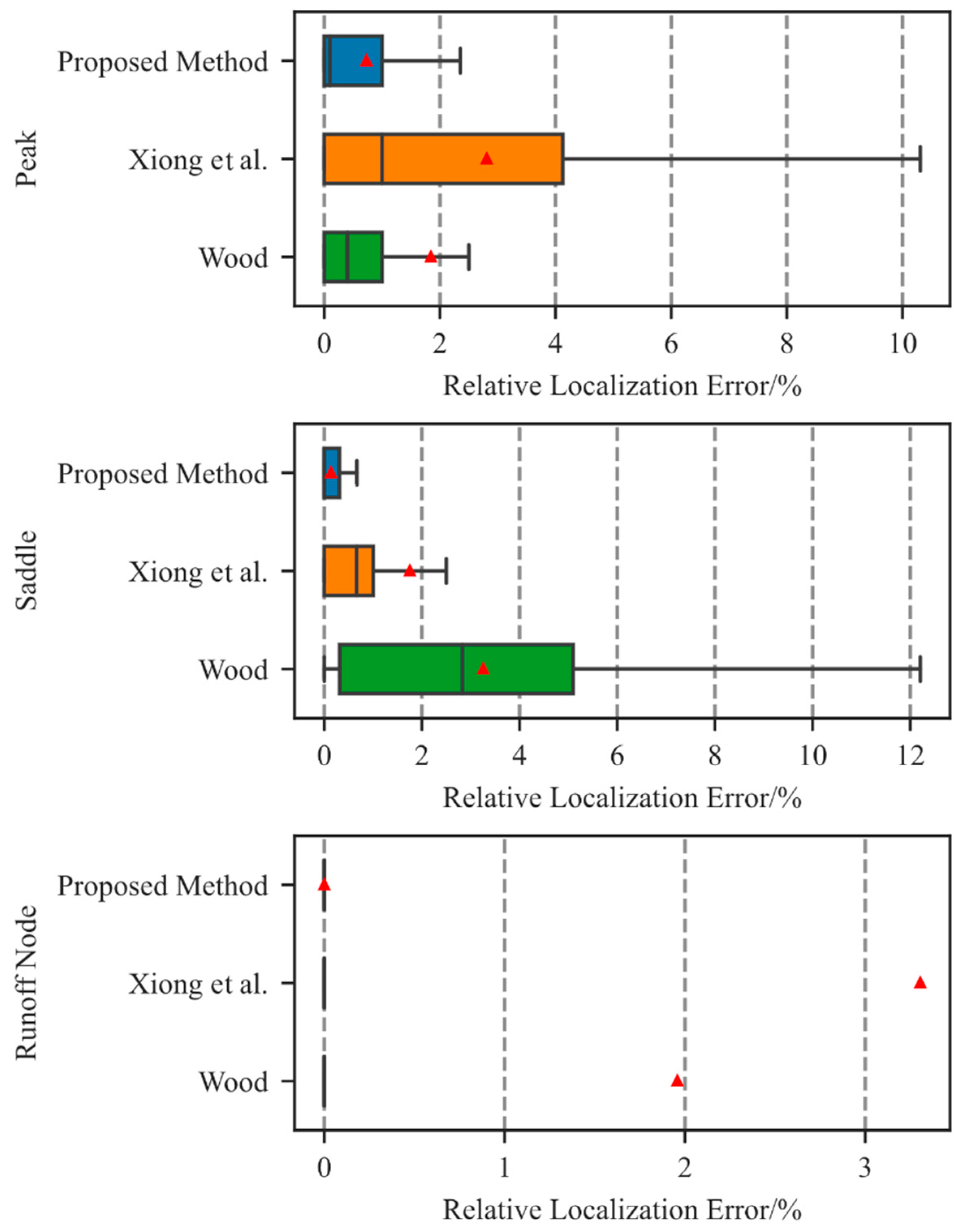
3.2. Extraction Results and Validations of Point Clusters

The integrated terrain feature-point clusters of six typical sample areas were extracted using the method proposed in Section 2. Since the typical sample areas are large, it is difficult to show the extraction effect directly, so the typical sample area is locally enlarged and the results are shown in Figure 8. It can be seen that the extracted peaks of the six typical sample areas are all located at the top of the slope, the saddles are mostly located between the two peaks and at the lowest local terrain, and the runoff nodes are all located in valleys. Theoretically, the three point clusters should be completely consistent. However, due to the DEM data’s spatial resolution and elevation accuracy, the three point clusters obtained based on the DEM data are not completely consistent. Therefore, the overall distribution of the extracted terrain feature elements is in line with expectations. Notably, the terrain segmentation threshold (i.e., the height difference from the peak to the saddle) is a vital threshold for extracting the peaks and their control areas by space segmentation, which is set to 40m here. The influence and significance of this threshold will be further discussed in Section 3.3 and Section 3.4 in this paper.

The extracted terrain feature-point clusters are overlaid with the ridgeline data and optical image data (Figure 8 and Figure 9, respectively) to verify the correctness and validity further. Figure 8 shows that the extracted peaks and saddles are mostly located on the ridgelines, and the runoff nodes are mostly located on the boundaries of the mountain control area. In addition, the saddles are mostly located in the saddle-shaped depression between two adjacent hills, and the runoff nodes are mostly located at the flat slope foot. Figure 9 shows that the extracted peaks are mostly located at the top of the slope, and the runoff nodes are mostly located in the valleys (such as roads, towns and cultivated land).

A quantitative evaluation of the extracted point clusters’ localization accuracy was performed. At present, it is still difficult to extract and verify the accuracy of terrain feature points. Due to the lack of standards such as the peak or the saddle, the peak extracted by each person is determined according to their own cognition, which cannot be well matched to the real world to determine the accuracy. This is one of the reasons why many researchers have done much work and tried to unify the understanding of topographic features [48,52,53]. As a result, this paper does not evaluate the absolute accuracy of the point clusters’ localization. Instead, we evaluate the relative localization accuracy of the point clusters from the perspective of element consistency. The relative localization errors of peaks and saddles are evaluated by the distance between the points and the nearest ridgelines, and the runoff nodes’ errors are assessed by the distance between the point and the boundaries of mountain control areas. For the extraction of terrain feature points, Wood proposed using the second derivative to obtain the six types of terrain feature points [54], which are widely used because of their simplicity and efficiency. Xiong et al. extracted peaks by searching the local maximum point of watershed boundaries based on the DEM data and achieved good results in the Tibetan Plateau [55]. Therefore, these two methods were performed to extract the terrain feature points in order to verify the relative position accuracy of the extracted point clusters with respect to others. The relative localization errors of the point clusters extracted from the six typical sample areas were calculated. The average localization errors are shown in

Table 2. Relative localization errors of extracted point clusters.

Point Cluster Type	Method Name	Avg./m	Std./m	PFM/%	PMM/%
Peak	Proposed Method	21.87	58.21	48.15	87.99
	Wood	55.32	112.68	37.63	73.38
	Xiong et al.	84.28	129.80	26.58	54.23
Saddle	Proposed Method	4.11	5.81	60.23	100.00
	Wood	97.68	103.81	20.20	37.66
	Xiong et al.	52.59	116.97	26.78	74.45
Runoff Node	Proposed Method	0.00	0.02	99.92	100.00
	Wood	58.74	291.74	88.31	92.81
	Xiong et al.	99.16	415.83	84.94	89.62

, and their distributions are shown by the boxplots (Figure 10). For the peak extraction, the proposed method’s average (avg.) and standard deviation (std.) values of localization error are 21.46 m and 54.08 m, respectively, which is less than half of the other methods; the percent of fully matching (PFM) (relative localization error of 0 m) of the proposed method is 47.32%, and the percent of mostly matching (PMM) (relative localization error less than or equal to the DEM spatial resolution) of the proposed method is 87.10%, nearly 50% higher than other methods. For the saddle extraction, the upper quartile and median value of the proposed method are close to 1/4 of the other methods; the average error is 4.11 m, close to 1/10 of the other methods. As for runoff node extraction, the PFM and the PMM are both close to 100%. In summary, the relative accuracy of the peak locations extracted using our method is better than the other methods. The saddles and runoff nodes extracted using our method have natural high consistency with the ridgelines and mountain control area boundaries, since they are extracted by intersecting the terrain feature lines. To sum up, the terrain feature points extracted by the proposed method not only have a good coupling relationship with each other, but also have high relative localization accuracy, which is consistent with geomorphological and hydrological cognition.

3.3. Statistics of Point Cluster Properties

The Height Difference between Peaks and Saddles (HDPS) is one of the main objects of interest in geomorphology research. The primary consideration of extracting terrain feature-point clusters using the integrated method is to determine a reasonable threshold of the HDPS. Considering the significant controversy regarding the quantitative indicators’ determination of mountain undulation, this study does not attempt to put forward a new quantitative indicator, but rather explores the influence and significance of the HDPS from the perspective of attribute statistics.

The HDPS has a significant influence on the extraction of peaks and their control areas, affecting the extraction of other terrain feature elements such as saddles and runoff nodes [31]. To quantitatively analyze the influence of the HDPS, taking these six typical sample areas as an example, each element in set $T=\left\{10n\right|n\in [1,40]\&n\in \mathbb{N}\}$ (unit: m) is used as the HDPS threshold to extract the terrain feature-point clusters, and the terrain feature-point clusters and their control areas with different HDPS thresholds are obtained. It is worth noting that the maximum value of the HDPS threshold of each typical sample area is different. This is due to the different elevation undulations in each area—some sample areas will not be able to extract the desired peaks and their control areas when the HDPS threshold exceeds a certain limit. The response of the mountain control area size and mountain undulation (the height difference between the peaks and the runoff nodes) to the HDPS changes is demonstrated using a scatter plot (Figure 11). The blue triangles in Figure 11 represent the response of the average mountain control area size to changes in the HDPS, and the blue dashed lines show the fitting relationship between them. For the typical sample areas, the HDPS and the average mountain control area size show a typical exponential relationship:

$$y=a{e}^{bx}$$

(7)

where y is the extracted average mountain control area size, x is the HDPS, and a and b are the fitting coefficients. Its minimum fitting coefficient of determination (R²) reaches 0.97. Observing the overall trend, it can be seen that with the gradual reduction of the topographic undulation (from the Qinling middle and high mountains to the loess hilly-gully), the fitting coefficient a gradually decreases, and the coefficient b gradually increases. Meanwhile, the orange dashed line in Figure 11 indicates the response of the average mountain undulation to changes in the HDPS, which shows a typical linear relationship:

$$y=cx+d$$

(8)

where y is the extracted average mountain undulation, x is the HDPS, c and d are the gradient and intercept of the regression line, respectively, and its average fitting R² reaches 0.94. Observing the overall trend, it can be seen that the regression lines’ intercept d shows a gradually increasing trend as the topographic undulation decreases.

The whole Shaanxi Province was used as the experimental sample area for analysis again to further verify the pattern of the fitting coefficients. The Shaanxi Province was divided into 123 grid cells according to the cell size of 0.5° × 0.5°, and each cell belonging to the geomorphological region was determined by the location for its centroid. The spatial distribution of these grid cells and the geomorphic zones they belong to were shown in Figure 12. Then, the terrain feature-point clusters were extracted again for each cell. The distribution probability histograms of the fitting coefficients were plotted (Figure 13) to analyze the relationships of the HDPS with mountain control area size and mountain undulation extracted from 123 grid cells grouped by geomorphological zones. As shown in Figure 13a and Figure 9b, the fitting coefficient a decreases with the decrease of topographic undulation as a whole, while the fitting coefficient b increases, which is consistent with the analysis results of the six typical sample areas. As shown in Figure 13d, the fitting coefficient d increases with the decrease of topographic undulation. In particular, there is no significant correlation between the fitting coefficients’ distribution and the landform types in the Guanzhong Plain and the Wind and Sand Transition Zone, which indicates that the HDPS is not effective in depicting the flat terrain and still needs further research. In summary, there are obviously exponential and linear correlations between the HDPS and mountain control area size and mountain undulation, respectively, and the fitting coefficients are greatly correlated with the landform types.

3.4. Point Cluster Properties and Geomorphological Regionalization

The relationship between the HDPS and mountain control area size and mountain undulation was analyzed above, and their fitting coefficients were found to be highly correlated with geomorphic zones. Therefore, further analyses were performed to validate the relationships between the point cluster properties and geomorphological zones. This paper’s study area is dominated by loess landforms [56]. There are many parameters that can measure the characteristics in the terrain analysis, but from another perspective, we could consider evaluating the cutting of the saddles and compare the differences between landscape types on this basis. Nir pointed out that the commonly used relative height is not a very good index, because even if the relative height was the same, the absolute height difference might also be different [57]. Likewise, when the relative height between the peak and the outlet is the same, the height difference between the saddles and peaks may also be different. Thus, here we define the Saddle Dissection Index:

$$SDI=(H_{peak}-H_{saddle})/(H_{peak}-H_{discharge})$$

(9)

where H_peak, H_saddle and H_discharge are defined as peak height, saddle height and the outlet height relative to the peak; thus, the SDI can be interpreted as the ratio between the HDPS and the degree of ups and downs.

Based on the terrain feature-point clusters extracted from the 0.5° × 0.5° grids of Shaanxi Province in Section 3.2, the HDPS and SDI of each peak are calculated. Then, the statistical attributes of each peak are interpolated using the natural neighborhood method to obtain the spatial distribution of the HDPS and SDI at 1 km spatial resolution in Shaanxi Province (Figure 14). As shown in Figure 14a, the statistical attributes of point clusters better reflect the overall characteristics of the terrain in Shaanxi Province, i.e., the topographic undulation shows an overall increasing trend from north to south. The topographic undulation in the Wind and Sand Transition Zone and Guanzhong Plain is low, the topographic undulation in Qinling and Daba Mountains is large, and the Loess Plateau is between them. In addition, the spatial distribution trend of the HDPS can be well distinguished from the Wind and Sand Transition Zone, the Loess Plateau, Guanzhong Plain and Qinling Mountain. The relatively weak portrayal appears between Guanzhong Plain and Qinling Mountain and Daba Mountain, which may be related to this region’s narrow distribution and complex topographic conditions. Figure 14b shows that the erosion in Shaanxi Province increases from south to north as a whole, and the northern part of the Loess Plateau is seriously eroded, showing a strong fragmentation trend, while the topography of the southern Loess Plateau and Guanzhong Plain is the most complete. The SDI can better distinguish the Loess Plateau, Guanzhong Plain and Qinling Mountains and the poorly carved area is the Hanzhong Basin. This may be due to the interaction of mountains around the basin, which leads to a certain fragmentation trend in the spatial trend of this region [58,59].

To sum up, the terrain feature-point clusters and their statistical attributes can reflect the fragmentation of the plane and mountains, and the stereoscopic undulation to a certain extent. At the same time, their results have a good correspondence with geomorphological divisions, which can serve for geomorphological classification and mapping. In general, the DEM we use has limited elevation accuracy and a large grid cell size. Research on the areas with less relief requires high-precision DEM data, such as LiDAR point cloud data. Therefore, under the condition of limited DEM accuracy, the ability to describe the landform of point clusters in the flat area is relatively weak, and further research is needed.

It is worth noting that terrain representation and various terrain-based geological analyses are significantly scale-dependent [60]. The scales of terrain analysis include geographic scale, observational scale, structural scale and analytical scale, all of which have scale effects [61,62]. For terrain feature extraction, the most significant is the analytical scale, i.e., what scale is used to extract the terrain features. To address this issue, the LLNV method was adopted to determine the optimal analysis scale in this paper. As for the scale, the effects caused by the geographic scale (i.e., the geographic extent of the study area) and the observational scale (i.e., the spatial resolution and height difference accuracy of the DEM data) need to be further researched using more data. On the other hand, this paper used morphological and runoff simulation methods to obtain integrated terrain feature-point clusters; according to Baker and Enzmann’s classification of geomorphologic features, the result is a feature point at the small-scale landform with an area about 10⁻³ to 10⁻¹ km² [63,64]. Further study is required for when the scale becomes larger, such as medium-scale tectonic units.

4. Conclusions

Terrain feature-point clusters determine the overall structure and characteristics of the terrain. They play a vital role in terrain representation and reconstruction, hydrological analysis of watersheds and other scientific studies and engineering applications. This work proposes an integrated extraction method for terrain feature-point clusters. Firstly, this method combines the morphological characteristics and runoff simulation to determine the best flow accumulation threshold quantitatively, and extracts the ridgelines based on this threshold. Then, the integrated terrain feature clusters are extracted using space segmentation and spatial analysis.

Experiments on six typical sample areas in Shaanxi Province show that the terrain feature-point clusters extracted by the proposed method are not only accurate in spatial position, but also have a good coupling relationship with each other, which is consistent with geomorphological and hydrological cognition. The point clusters’ attribute statistics show that there is an exponential dependency y = ae^bx and a linear dependency y = cx+d of the mountain control area size, and of the mountain undulation, respectively, from the HDPS. Meanwhile, the fitting coefficients have a great correlation with the landform types. The fitting coefficient a decreases with the decrease of terrain undulation as a whole, while the coefficients b and d increase. In addition, there is a good correspondence between the spatial distribution trend of point cluster attributes and the geomorphological zoning boundaries of Shaanxi Province.

In summary, the point cluster extraction results of the proposed method are consistent with geomorphological cognition, and their attributes have important geomorphological significance, which can serve for geomorphological zoning and mapping. However, due to the limitations of DEM data accuracy and topographic undulation size, the terrain feature-point clusters are relatively poorly depicted in plain areas, which needs further research.

References

1. Peizhi, H.; Lai, P.-C. The Derivation of Skeleton Lines for Terrain Features. Geo-Spatial Inf. Sci. 2002, 5, 68–73. [Google Scholar] [CrossRef] [Green Version]
2. Li, M.; Wu, T.; Li, W.; Wang, C.; Dai, W.; Su, X.; Zhao, Y. Terrain Skeleton Construction and Analysis in Loess Plateau of Northern Shaanxi. ISPRS Int. J. Geo-Inf. 2022, 11, 136. [Google Scholar] [CrossRef]
3. Li, S.; Hu, G.; Cheng, X.; Xiong, L.; Tang, G.; Strobl, J. Integrating Topographic Knowledge into Deep Learning for the Void-Filling of Digital Elevation Models. Remote Sens. Environ. 2022, 269, 112818. [Google Scholar] [CrossRef]
4. Syzdykbayev, M.; Karimi, B.; Karimi, H. A Method for Extracting Some Key Terrain Features from Shaded Relief of Digital Terrain Models. Remote Sens. 2020, 12, 2809. [Google Scholar] [CrossRef]
5. Wang, L.; Liu, H. An Efficient Method for Identifying and Filling Surface Depressions in Digital Elevation Models for Hydrologic Analysis and Modelling. Int. J. Geogr. Inf. Sci. 2006, 20, 193–213. [Google Scholar] [CrossRef]
6. Lv, G.; Xiong, L.; Chen, M.; Tang, G.; Sheng, Y.; Liu, X.; Song, Z.; Lu, Y.; Yu, Z.; Zhang, K.; et al. Chinese Progress in Geomorphometry. J. Geogr. Sci. 2017, 27, 1389–1412. [Google Scholar] [CrossRef]
7. Yang, X.; Tang, G.; Meng, X.; Xiong, L. Saddle Position-Based Method for Extraction of Depressions in Fengcong Areas by Using Digital Elevation Models. ISPRS Int. J. Geo-Inf. 2018, 7, 136. [Google Scholar] [CrossRef] [Green Version]
8. Hu, J.; Tang, M.; Luo, M.; Wei, L.; Yan, Z.; Qin, Z. The extraction of characteristic elements of mountain based on DEM. J. Geo-Inf. Sci. 2020, 22, 422–430. [Google Scholar]
9. Xiong, L.; Tang, G.; Yang, X.; Li, F. Geomorphology-Oriented Digital Terrain Analysis: Progress and Perspectives. J. Geogr. Sci. 2021, 31, 456–476. [Google Scholar] [CrossRef]
10. Chen, Z.-T.; Guevara, J.A. Systematic Selection of Very Important Points (VIP) from Digital Terrain Model for Constructing Triangular Irregular Networks. Auto Cart. 1987, 8, 50–56. [Google Scholar]
11. Gökgöz, T.; Hacar, M. Comparison of Two Methods for Multiresolution Terrain Modelling in GIS. Geocarto Int. 2020, 35, 1360–1372. [Google Scholar] [CrossRef]
12. Cayley, A. On Contour and Slope Lines. Lond. Edinb. Dublin Philos. Mag. J. Sci. 1859, 18, 264–268. [Google Scholar] [CrossRef]
13. Maxwell, J.C. On Hills and Dales: To the Editors of the Philosophical Magazine and Journal. Lond. Edinb. Dublin Philos. Mag. J. Sci. 1870, 40, 421–427. [Google Scholar] [CrossRef]
14. Morse, M.; Cairns, S.S. Critical Point Theory in Global Analysis and Differential Topology; Academic Press: Cambridge, MA, USA, 1969. [Google Scholar]
15. Matsumoto, Y. An Introduction to Morse Theory; American Mathematical Society: Washington, DC, USA, 2002; Volume 208. [Google Scholar]
16. Robins, V.; Wood, P.J.; Sheppard, A.P. Theory and Algorithms for Constructing Discrete Morse Complexes from Grayscale Digital Images. IEEE Trans. Pattern Anal. Mach. Intell. 2011, 33, 1646–1658. [Google Scholar] [CrossRef]
17. Čomić, L.; De Floriani, L.; Iuricich, F.; Magillo, P. Computing a Discrete Morse Gradient from a Watershed Decomposition. Comput. Graph. 2016, 58, 43–52. [Google Scholar] [CrossRef] [Green Version]
18. Takahashi, S.; Ikeda, T.; Shinagawa, Y.; Kunii, T.L.; Ueda, M. Algorithms for Extracting Correct Critical Points and Constructing Topological Graphs from Discrete Geographical Elevation Data. In Proceedings of the Computer Graphics Forum; Wiley Online Library: Hoboken, NJ, USA, 1995; Volume 14, pp. 181–192. [Google Scholar]
19. Pfaltz, J.L. Surface Networks. Geogr. Anal. 1976, 8, 77–93. [Google Scholar] [CrossRef]
20. Wood, E.F.; Sivapalan, M.; Beven, K.; Band, L. Effects of Spatial Variability and Scale with Implications to Hydrologic Modeling. J. Hydrol. 1988, 102, 29–47. [Google Scholar] [CrossRef]
21. Deng, Y.; Wilson, J.P.; Bauer, B.O. DEM Resolution Dependencies of Terrain Attributes Across a Landscape. Int. J. Geogr. Inf. Sci. 2007, 21, 187–213. [Google Scholar] [CrossRef]
22. Magillo, P.; Danovaro, E.; De Floriani, L.; Papaleo, L.; Vitali, M. A Discrete Approach to Compute Terrain Morphology. In Proceedings of the Computer Vision and Computer Graphics. Theory and Applications; Braz, J., Ranchordas, A., Araújo, H.J., Pereira, J.M., Eds.; Springer: Berlin/Heidelberg, Germany, 2008; pp. 13–26. [Google Scholar]
23. Aumann, G.; Ebner, H.; Tang, L. Automatic Derivation of Skeleton Lines from Digitized Contours. ISPRS J. Photogramm. Remote Sens. 1991, 46, 259–268. [Google Scholar] [CrossRef]
24. Liu, H.; Jin, H.; Miao, B. An Algorithm for Extracting Terrain Structure Lines Based on Contour Data. In Proceedings of the Sixth International Symposium on Digital Earth: Models, Algorithms, and Virtual Reality, Beijing, China, 9–12 September 2009; Volume 7840, pp. 286–291. [Google Scholar]
25. Kong, Y.; Su, J.; Zhang, Y. A New Method of Extracting Terrain Feature Lines by Morphology. Information 2012, 15, 2585–2591. [Google Scholar]
26. O’Callaghan, J.F.; Mark, D.M. The Extraction of Drainage Networks from Digital Elevation Data. Comput. Vis. Graph. Image Process. 1984, 28, 323–344. [Google Scholar] [CrossRef]
27. Bakula, K.; Kurczynski, Z. The Role of Structural Lines Extraction from High-Resolution Digital Terrain Models in the Process of Height Data Reduction. In Proceedings of the Geoconference on Informatics, Geoinformatics and Remote Sensing-Conference Proceedings; Stef92 Technology Ltd.: Sofia, Bulgaria, 2013; Volume I, pp. 579–586. [Google Scholar]
28. Zhang, S.; Zhao, B.; Erdun, E. Watershed Characteristics Extraction and Subsequent Terrain Analysis Based on Digital Elevation Model in Flat Region. J. Hydrol. Eng. 2014, 19, 04014023. [Google Scholar] [CrossRef]
29. Jenson, S.K.; Domingue, J.O. Extracting Topographic Structure from Digital Elevation Data for Geographic Information System Analysis. Photogramm. Eng. Remote Sens. 1988, 54, 1593–1600. [Google Scholar]
30. Ariza-Villaverde, A.B.; Jiménez-Hornero, F.J.; Gutiérrez de Ravé, E. Influence of DEM Resolution on Drainage Network Extraction: A Multifractal Analysis. Geomorphology 2015, 241, 243–254. [Google Scholar] [CrossRef]
31. Ma, Y.; Song, Y.; Zhang, W.; Kang, X.; Zhao, P. Method of Peak Extraction Based on Spatial Subdivision. J. Geomat. Sci. Technol. 2015, 32, 433–436, 440. [Google Scholar]
32. Li, S.; Xiong, L.; Tang, G.; Strobl, J. Deep Learning-Based Approach for Landform Classification from Integrated Data Sources of Digital Elevation Model and Imagery. Geomorphology 2020, 354, 107045. [Google Scholar] [CrossRef]
33. Luo, M.; Tang, G. Mountain peaks extraction based on geomorphology cognitive and space segmentation. Sci. Surv. Mapp. 2010, 35, 126–127, 253. [Google Scholar] [CrossRef]
34. Vincent, L.; Soille, P. Watersheds in Digital Spaces: An Efficient Algorithm Based on Immersion Simulations. IEEE Trans. Pattern Anal. Mach. Intell. 1991, 13, 583–598. [Google Scholar] [CrossRef] [Green Version]
35. Meyer, F. Topographic Distance and Watershed Lines. Signal Process. 1994, 38, 113–125. [Google Scholar] [CrossRef]
36. Roerdink, J.B.T.M.; Meijster, A. The Watershed Transform: Definitions, Algorithms and Parallelization Strategies. Fundam. Inform. 2000, 41, 187–228. [Google Scholar] [CrossRef] [Green Version]
37. Stoev, S.L.; Strasser, W. Extracting Regions of Interest Applying a Local Watershed Transformation. In Proceedings of the Proceedings Visualization 2000, Salt Lake City, UT, USA, 8–13 October 2000; pp. 21–28. [Google Scholar]
38. Liu, Y.; Xiong, L.; Fang, X. Pattern Analysis of Terrain Feature Points of Loess Topography. Geogr. Geo-Inf. Sci. 2017, 33, 35–41. [Google Scholar]
39. Liu, D. Preparation of small-scale stratified color topographic maps. Acta Geogr. Sin. 1957, 23, 447–458. [Google Scholar] [CrossRef]
40. Zhou, Y. Investigation of Loess Positive and Negative Terrain Based on DEMs; Nanjing Normal University: Nanjing, China, 2008. [Google Scholar]
41. Tang, G.; Liu, X.; Lv, G. Tutorials of Digital Elevation Models; Science Press: Beijing, China, 2016. [Google Scholar]
42. Martha, T.R.; Vamsee, A.M.; Tripathi, V.; Kumar, K.V. Detection of Coastal Landforms in a Deltaic Area Using a Multi-Scale Object-Based Classification Method. Curr. Sci. 2018, 114, 1338–1345. [Google Scholar] [CrossRef]
43. Lin, X.; Wen, J.; Liu, Q.; Xiao, Q.; You, D.; Wu, S.; Hao, D.; Wu, X. A Multi-Scale Validation Strategy for Albedo Products over Rugged Terrain and Preliminary Application in Heihe River Basin, China. Remote Sens. 2018, 10, 156. [Google Scholar] [CrossRef] [Green Version]
44. Woodcock, C.E.; Strahler, A.H. The Factor of Scale in Remote Sensing. Remote Sens. Environ. 1987, 21, 311–332. [Google Scholar] [CrossRef]
45. Drăguţ, L.; Eisank, C.; Strasser, T. Local Variance for Multi-Scale Analysis in Geomorphometry. Geomorphology 2011, 130, 162–172. [Google Scholar] [CrossRef] [Green Version]
46. Li, J.; Zhang, H.; Xu, E. A Two-Level Nested Model for Extracting Positive and Negative Terrains Combining Morphology and Visualization Indicators. Ecol. Indic. 2020, 109, 105842. [Google Scholar] [CrossRef]
47. Fisher, P.; Wood, J.; Cheng, T. Where Is Helvellyn? Fuzziness of Multi-scale Landscape Morphometry. Trans. Inst. Br. Geogr. 2004, 29, 106–128. [Google Scholar] [CrossRef]
48. Schmidt, J.; Hewitt, A. Fuzzy Land Element Classification from DTMs Based on Geometry and Terrain Position. Geoderma 2004, 121, 243–256. [Google Scholar] [CrossRef]
49. López-Vicente, M.; Álvarez, S. Influence of DEM Resolution on Modelling Hydrological Connectivity in a Complex Agricultural Catchment with Woody Crops. Earth Surf. Process. Landf. 2018, 43, 1403–1415. [Google Scholar] [CrossRef]
50. Zhan, C. A Hybrid Line Thinning Approach. In Proceedings of the Auto-Carto; American Society for Photogrammetry and Remote Sensing: Minneapolis, MN, USA, 1993; p. 396. [Google Scholar]
51. Band, L.; Robinson, V. Intelligent Land Information System Final Report; Toronto University: Toronto, ON, Canada, 1992. [Google Scholar]
52. Smith, B.; Mark, D.M. Do Mountains Exist? Towards an Ontology of Landforms. Environ. Plan. B Plan. Des. 2003, 30, 411–427. [Google Scholar] [CrossRef] [Green Version]
53. Zhu, L.-J.; Zhu, A.-X.; Qin, C.-Z.; Liu, J.-Z. Automatic Approach to Deriving Fuzzy Slope Positions. Geomorphology 2018, 304, 173–183. [Google Scholar] [CrossRef]
54. Wood, J. The Geomorphological Characterisation of Digital Elevation Models. Ph.D. Thesis, University of Leicester, Leicester, UK, 1996. [Google Scholar]
55. Xiong, L.-Y.; Tang, G.-A.; Zhu, A.-X.; Qian, Y.-Q. A Peak-Cluster Assessment Method for the Identification of Upland Planation Surfaces. Int. J. Geogr. Inf. Sci. 2017, 31, 387–404. [Google Scholar] [CrossRef]
56. Cheng, Y.; Li, J.; Xiong, L.; Tang, G. Clustering Gully Profiles for Investigating the Spatial Variation in Landform Formation on the Chinese Loess Plateau. J. Mt. Sci. 2021, 18, 2742–2760. [Google Scholar] [CrossRef]
57. Nir, D. The Ratio of Relative and Absolute Altitudes of Mt. Carmel: A Contribution to the Problem of Relief Analysis and Relief Classification. Geogr. Rev. 1957, 47, 564–569. [Google Scholar] [CrossRef]
58. Cheng, W.; Zhou, C.; Li, B.; Sheng, Y. Geomorphological regionalization theory system and division methodology of China. Acta Geogr. Sin. 2019, 74, 839–856. [Google Scholar]
59. Wang, N.; Cheng, W.; Wang, B.; Liu, Q.; Zhou, C. Geomorphological Regionalization Theory System and Division Methodology of China. J. Geogr. Sci. 2020, 30, 212–232. [Google Scholar] [CrossRef]
60. Lam, N.S.-N. Fractals and Scale in Environmental Assessment and Monitoring. Scale Geogr. Inq. Nat. Soc. Method 2004, 23–40. [Google Scholar] [CrossRef]
61. Lam, N.S.-N.; Quattrochi, D.A. On the Issues of Scale, Resolution, and Fractal Analysis in the Mapping Sciences. Prof. Geogr. 1992, 44, 88–98. [Google Scholar] [CrossRef]
62. Cao, C.; Lam, N.S.-N. Understanding the Scale and Resolution Effects in Remote Sensing and GIS. Scale Remote Sens. GIS 1997, 57, 72. [Google Scholar]
63. Enzmann, R.D. Geomorphylogy-Expanded Theory; Fairbridge, R.W., Ed.; The Encyclopedia of Geomorphology, Reinhold Book Corporation: New York, NY, USA, 1968. [Google Scholar]
64. Baker, V.R. Introduction: Regional Landform Analysis; Short, N.M., Blair, R.R., Eds.; Geomorphology from Space, A Global Overview of Regional Landforms; NASA: Washington, DC, USA, 1986. [Google Scholar]
Figure 1. Principle of the integrated point cluster extraction: the black triangles, green squares and blue dots represent peaks, saddles and runoff nodes, respectively; the red lines represent ridgelines, and the black dashed boxes represent the mountain control areas.
Remotesensing 14 02776 g001
Figure 2. Study area and typical sample areas: (a) the overview of the study area; (b) the locations of the six typical sample areas in the DEM imageries.
Remotesensing 14 02776 g002
Figure 3. Processes of the positive terrain-constrained ridgeline extraction.
Remotesensing 14 02776 g003
Figure 4. Processes of the terrain feature-point cluster extraction [33].
Remotesensing 14 02776 g004
Figure 5. Correspondence between peaks and saddles in original and anti-terrain: (a) the peaks and saddles in the original terrain; (b) the peaks and saddles in the corresponding anti-terrain.
Remotesensing 14 02776 g005
Figure 6. The response of the LLNV and potential ridgelines’ length to changes in the window size of neighborhood analysis and flow accumulation threshold, respectively: the blue triangles represent the response of the LLNV to changes in the window size of the neighborhood analysis, the blue dashed lines represent the quadratic polynomial regression curves of the two, and the blue vertical dashed lines represent the optimal window sizes of the neighborhood analysis obtained by the proposed method. The orange stars represent the response of the extracted ridgeline’s length to changes in flow accumulation thresholds in the runoff simulation, and the orange dashed lines represent the logistic regression curves of the two.
Remotesensing 14 02776 g006
Figure 7. The results of positive terrain extracted with different window sizes of neighborhood analysis in Ningshan County: (af) the positive terrain distribution of Ningxia County extracted with different window sizes of neighborhood analysis. The positive terrain areas are shown as blue, the upper left corners are the window sizes of these subplots, the analysis window sizes from subplot (a) to subplot (f) are 3, 11, 21, 31, 41 and 51, respectively. Among them, subplot (c) shows positive terrain distribution corresponding to the optimal analysis window size (s = 21) extracted using the proposed method.
Remotesensing 14 02776 g007
Figure 8. Validation of extracted point clusters by the ridgelines: (af) correspond to six typical sample areas, including Hanyin, Mizhi, Ningshan, Yanchuan, Zhen’an and Zhenba County, respectively; the black triangles, purple squares and blue dots represent peaks, saddles and runoff nodes, respectively; the yellow lines represent ridgelines, and the black dashed boxes represent the mountain control areas.
Remotesensing 14 02776 g008
Figure 9. Validation of extracted point clusters by the optical image data: (af) correspond to six typical sample areas, including Hanyin, Mizhi, Ningshan, Yanchuan, Zhen’an and Zhenba County, respectively; the black triangles, purple squares and blue dots represent peaks, saddles and runoff nodes, respectively.
Remotesensing 14 02776 g009
Figure 10. Relative localization error distribution of extracted point clusters: the different colored boxes represent different methods; the upper and lower quartiles of the data are depicted by the box’s upper and lower boundaries, respectively; the median and average values are depicted by the inner horizontal lines and the red triangles, respectively; the whiskers extending from the ends of the boxes are used to represent variables other than the upper and lower quartiles.
Remotesensing 14 02776 g010
Figure 11. Response of mountain control area size and mountain undulation to HDPS changes in the six typical sample areas: the blue triangles represent the relationship between the HDPS and the mountain control area size; the orange stars represent the relationship between the HDPS and the mountain undulation; the blue and orange dashed lines represent the regression curves of the two.
Remotesensing 14 02776 g011
Figure 12. Spatial distribution of grid cells in Shaanxi Province: the blue dot represents the centroid of each gird; colored rectangles indicate the spatial extent of these cells, and different colors are adopted for different geomorphological regions.
Remotesensing 14 02776 g012
Figure 13. Relationship between the HDPS and mountain control area size and mountain undulation in each sample area of Shaanxi Province: (a,b) the coefficient distribution histogram of the exponential regression between the HDPS and the mountain control area size; (c,d) the coefficient distribution histogram of the linear regression between the HDPS and the mountain undulation, while coefficient c and d are the gradient and intercept of the regression line, respectively; six colors in the figures correspond to six geomorphological zones in Shaanxi Province.
Remotesensing 14 02776 g013
Figure 14. Spatial distribution of the HDPS and SDI: (a) spatial distribution of the HDPS in Shaanxi Province; (b) spatial distribution of the SDI in Shaanxi Province.
Remotesensing 14 02776 g014