Abstract
There is consistent evidence of vegetation greening in Central Asia over the past four decades. However, in the early 1990s, the greening temporarily stagnated and even for a time reversed. In this study, we evaluate changes in the normalized difference vegetation index (NDVI) based on the long-term satellite-derived remote sensing data systems of the Global Inventory Modelling and Mapping Studies (GIMMS) NDVI from 1981 to 2013 and MODIS NDVI from 2000 to 2020 to determine whether the vegetation in Central Asia has browned. Our findings indicate that the seasonal sequence of NDVI is summer > spring > autumn > winter, and the spatial distribution pattern is a semicircular distribution, with the Aral Sea Basin as its core and an upward tendency from inside to outside. Around the mid-1990s, the region’s vegetation experienced two climatic environments with opposing trends (cold and wet; dry and hot). Prior to 1994, NDVI increased substantially throughout the growth phase (April–October), but this trend reversed after 1994, when vegetation began to brown. Our findings suggest that changes in vegetation NDVI are linked to climate change induced by increased CO2. The state of water deficit caused by temperature changes is a major cause of the browning turning point across the study area. At the same time, changes in vegetation NDVI were consistent with changes in drought degree (PDSI). This research is relevant for monitoring vegetation NDVI and carbon neutralization in Central Asian ecosystems.
1. Introduction
Vegetation is an important part of ecosystems, so exploring changes in vegetation health is vital to monitoring vegetation growth within a region [1]. Central Asia is home to an arid and highly seasonal steppe-desert biome [2] whose ecosystem makes up a relatively large part of the land cover area. Due to the limitations of ground-based observation techniques, most studies have been conducted in conjunction with remote sensing techniques [3]. Of the various spectral indicators extracted from the satellite data, a commonly used and well-understood vegetation index is the normalized difference vegetation index (NDVI) [4,5,6]. The index is a parameter for describing the quantity and quality of vegetation growth and biomass [7]. The results of related studies show that NDVI combined with remote sensing data can effectively reflect the growth status of vegetation, the degree of cover, and its change pattern [8,9]. Previous studies have shown that areas with a multiyear (1982–2020) average NDVI < 0.1 are not included and are generally considered barren [10,11].
Several studies have recently been conducted using remote sensing monitoring of vegetation in some typical regions, such as the arid zones of Central Asia, the Tibetan Plateau, and the East African Plateau, and even on a global scale. The three main ones are: (1) a comparative study on the differences and science of the products themselves [4,12]; (2) analysis of vegetation dynamics and evolution studies [13,14]; and (3) simulation and mechanistic analysis of climate change, water resource change, and ecosystem assessment using vegetation indices as parameters [5,14,15]. Even though some of these studies focus on the arid zones of Central Asia, they do not fully exploit remote sensing data to examine the long-term evolution of the area’s vegetation and the factors that influence it. Therefore, the current research is more thorough in the context of NDVI across the Central Asian landscape.
Temperature, precipitation, humidity, air pressure, CO2, and light all influence vegetation growth, with temperature and precipitation playing the most critical roles [16]. From 1982 to 2012, Liu Y. [17] found that global vegetation NDVI was gradually reduced by warmth and steadily raised by precipitation. In a study on increased greening of vegetation in the Hay River Basin, CO2 was found to be the most significant contributor to the NDVI trend (45%), followed by human activities (mean contribution of 27%) [6]. Studies on factors influencing vegetation change in the Central Asian Tien Shan show that vegetation in this region is extremely sensitive to moisture deficit, and that soil moisture deficit has a greater impact on vegetation change than does high water vapor pressure deficit [1].
The effects of drought can be expressed in vegetation as a range of physiological responses and time scales, with drought’s impact on vegetation being a more integrated indicator [18,19]. When compared with surface temperature and water layer thickness, NDVI has the strongest correlation with drought for most vegetation types [19,20]. Three satellite series’ NDVI (MODIS, Landsat, and Sentinel-2) were calculated and found to be closely connected to drought [21]. Using sensors in tandem offers the greatest possible representation of canopy health during acute drought occurrences [21].
In a research study conducted by Myneni et al. (1997) [22], who used NDVI data from 1981 to 1991, a large-scale growth trend in vegetation greenness was revealed throughout the Northern Hemisphere. In the same study area, in studies investigating the seasonal response of Northern Hemisphere vegetation to climate change (1982–2013), the authors found that the increasing tendency of greenness was stalled and even shifted to vegetation browning after 1994–1997, particularly in Central Europe, Northern North America, and Central Siberia [23]. In Pan’s research, the results unanimously show the expansion and acceleration of a browning trend since 1994 [24]. After the late 1990s, the browning trend increased across all latitudes of the Northern Hemisphere. This growth is particularly evident in the northern middle and low latitudes, where the greening trend stagnated or even reversed [24]. In the Belt and Road area, the temporal trend of vegetation in 1981–2016 indicated an obvious trend change that mainly occurred in 2000. After the turning point (i.e., 1994), the browning trend was extended and enhanced to a large extent in Eastern Europe and Central Asia, occurring primarily around the turn of the millennium [25].
The existing research results show that there are differences in the influencing factors of vegetation NDVI change across different regions, and that the main influencing factors also differ across time periods. Furthermore, NDVI data sources are relatively singular, and there is no comparison of possible temporal and spatial differences of multiple data sources. This study, on the other hand, uses multiple data sources to analyze and couple the synergistic impact of multiple factors on NDVI changes. Investigating the change pattern of vegetation NDVI and its influencing factors based on long time series and high-resolution remote sensing data is critically important in light of the accelerated climate change.
Central Asia lies at the junction of Asia and Europe [26]. It is also located in a world-class arid zone with sparse surface vegetation and severe water scarcity [27]. It comprises a typical temperate desert and steppe arid zone, with a relatively fragile ecological environment [28,29,30]. In the context of global warming, climate change is dramatic and ecosystems are fragile [31]. In the post-Soviet era, ecological degradation, such as grassland degradation and lake shrinkage, such as the Aral Sea crisis, occurred in parts of Central Asia, mainly due to the chaotic ecological management systems of the five Central Asian countries [32,33]. In particular, in the context of climate change, the increase in temperature and drought will directly change the growth state of mountain–oasis–desert vegetation in Central Asia, which in turn will affect the spatial and temporal distribution of vegetation NDVI [34,35]. The ecological and environmental problems in Central Asia have increased significantly in the course of the ongoing disturbance of global climate change and the intensification of human activities. In addition, due to its special geographic conditions, the area has become an important channel for the construction of China’s “One Belt, One Road” [36].
The significance of Central Asia’s political and economic standing, as well as the reality of its environmental challenges, necessitates that we pay attention to its ecological features, the quality of which is mostly reflected in changes in vegetation NDVI [37]. Because of this, the present study uses remote sensing image data to analyze vegetation changes in Central Asia from the 1980s onwards and discusses the influencing factors in terms of environmental factors to understand the impact of drought and climate change on vegetation dynamics. The study is important for providing a reference for ecological conservation and future development planning in Central Asia.
2. Study Area
The study area covers Central Asia, which is positioned deep in the hinterland of the Eurasian continent. It spans 46°29′–87°18′E from east to west and 35°07′–55°26′N from north to south, covering a total area of about 4 × 10⁶ km2. The administrative regions within this boundary include Kazakhstan (Kaz), Turkmenistan (TKM), Uzbekistan (UZB), Kyrgyzstan (KGZ), and Tajikistan (TJK) (Figure 1).
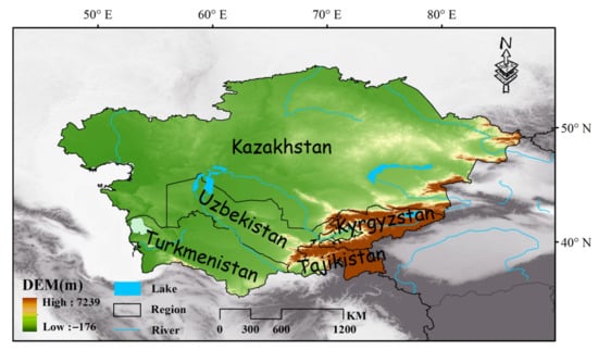
Figure 1.
Study area. No. GS (2016) 2966.
Across Central Asia, there is a gradual rise in altitude from the plains in the west to the mountains in the east, with the highest altitude being the Communist Peak at 7495 m. The high mountainous areas of the Pamir region of Tajikistan and the Tien Shan region in western Kyrgyzstan have on average an elevation of 4000–5000 m. Central Asia is dominated by plains, hills, rolling hills, and extensive desert areas. The climatic types include temperate desert climate, temperate steppe climate, and highland mountain climate, with a transition from semiarid to arid zones from north to south. Annual precipitation is about 200 mm in northern Central Asia and up to 1000 mm in the southern mountain ranges, with the highest precipitation in June and July in the high-altitude mountains. In general, the average annual precipitation is sparse in Central Asia, but there is a high temporal and spatial variability in precipitation. In terms of temperature, it is lower in the north than in the south and lower in the east than in the west, with the average temperature in July ranging from 32 °C in the south to 25 °C in the north, with a large daily difference in temperature and cold air moving south in winter, with the average temperature in January being 3 °C in the south and −15 °C in the north. Most of the region is grassland, which accounts for up to 85.73% of the study area.
3. Data
3.1. Satellite Data
3.1.1. GIMMS NDVI
We selected NDVI product data from Global Inventory Modelling and Mapping Studies (GIMMS) remote sensing products [38]. The GIMMS NDVI dataset was generated by several AVHRR sensors from NOAA for a global 1/12th degree (~8 km) latitude/grid. The latest version of the dataset is NDVI3g (third-generation GIMMS NDVI from AVHRR sensors). It covers half-month intervals from July 1981 to December 2013. The GIMMS NDVI3g dataset has been corrected for calibration, volcanic aerosols, orbital drift effects, and view geometry. Its data processing objectives are aimed at improving data quality at high latitudes to facilitate studies of vegetation activity changes in Northern Hemisphere ecosystems (Table 1).

Table 1.
GIMMS and MODIS data products.
3.1.2. MODIS NDVI
The global MODIS vegetation index is designed to provide consistent spatial and temporal comparisons of vegetation status. The MODIS MOD13A2 V6.1 product [39] complements NOAA’s Advanced Very High Resolution Radiometer (AVHRR) NDVI product by providing time series continuity for the application of vegetation index products. As a grid level 3 product used in sinusoidal projections to show land cover and its changes, in addition to being used for global vegetation condition monitoring, these data can be employed as input to global biogeochemical and hydrological processes as well as global and regional climate modelling. They can also be used as a simulation of global biogeochemical, meteorological, and hydrological processes, including land surface biophysical properties, primary production, and land cover conversion.
MODIS NDVI (MOD13A2) provides global-scale data every 16 days at a spatial resolution of 1 km, with accuracy assessed over a wide range of locations and periods. Currently updated from February 2000 to December 2021, the data are already available for use in scientific publications, although improved versions may be available later (Table 1).
3.2. Climate Data
The actual water vapor pressure (VAP), water vapor pressure difference (VPD), potential evapotranspiration (PET), precipitation (PRE), soil moisture (SM), and Palmer Drought Severity Index (PDSI) are from the TerraClimate reanalysis data from 1981 to 2020. The VAP and VPD were further calculated to obtain saturated water vapor pressure (VSP) and selected air temperature (TEM) data from the fifth-generation European Centre for Medium-Range Weather Forecasts reanalysis of the global climate (ERA5) [40]. ERA5 TEM data are derived from a combination of models and observations as they overcome the limitations of existing station records in terms of length and spatial coverage [41]. Since the spatial resolution of the TerraClimate reanalysis data is 4638.3 m, the ERA5 TEM data with a spatial resolution of 0.1° were kriged to a raster of 4638.3 m, thus unifying the spatial resolution (Table 2).
Table 2.
TerraClimate and ERA5 data products.
4. Methodology
4.1. VSP Calculation
Saturated water vapor pressure (VSP) [42] is calculated based on VAP and VPD reanalysis data products of TerraClimate [43], as follows:
4.2. Piecewise Regression Analysis
The abnormal turning point of NDVI in the growth period based on GIMMS in Central Asia is identified by the piecewise regression model, which has been widely used in NDVI and climate analysis [1,24,44].
4.3. Trend Algorithm
In this paper, variables from the past several years are simulated and analyzed year by year and month by month based on the unary linear regression method. The dynamic changes over the years are then analyzed. For example, to study the spatiotemporal variation trend of the variables grid by grid, the linear regression coefficient trend of the variable was calculated as:
where n and j are the lengths of the time series and the j year of the time series, respectively, and Pj is the mean value of the variable in the j year. Trend > 0 indicates that the variable is increasing over time, and Trend < 0 indicates that the variable is decreasing over time. The present study classifies the variable trend to indicate the degree of trend on the variable time scale. For all analyses, a significance level of 0.05 was used (i.e., if one of the analyses yields a p-value < 0.05, the null hypothesis is rejected). Here, the calculation of p-value is obtained by F-test using this formula:
where r is the correlation coefficient and n are the number of samples.
4.4. Correlation Analysis
At the same time, the Pearson correlation coefficient [45,46] was used to further analyze the correlation between x and y. The formula is:
where n is the length of time series, Xi and Yi represent variable value, and and represent the multiyear mean of variable value. When R ∈ [0, 1], a positive correlation is indicated, but when R ∈ [–1, 0], a negative correlation is represented. Further, when R = 1, X and Y are completely positively correlated; when R = −1, X and Y are completely negatively correlated; and when R = 0, X and Y are unrelated. For correlation, we employed the p-value to test using a threshold of p < 0.05. Here, the calculation of the p-value is obtained by t-test using this formula:
where r is the correlation coefficient and n denotes the number of samples.
5. Results
5.1. Spatial and Temporal Variation Trends of NDVI in Central Asia
In this study, the high-value areas of NDVI spatial distribution are concentrated in the northern hilly areas and the eastern and southern mountain areas, while the low-value areas (NDVI < 0.1) are concentrated in the southwest, which has the Karakum and Kyzylkum Deserts. The overall spatial law is a semicircular distribution pattern, with the Aral Sea Basin at the center and an upward trend from inside to outside. Meanwhile, the spatial distribution pattern of NDVI and its mean value of GIMMS and MODIS is calculated for different seasons. As well, the spatial changes of different NDVI products in different seasons are compared. We found that the spatial range of NDVI for various products shows the temporal change of summer > spring > autumn > winter. Overall, MODIS NDVI is lower than GIMMS NDVI, but the spatial variation law of NDVI for various products is essentially the same in seasons within the year, resulting in a semicircular distribution pattern, with the Aral Sea Basin at its core and an upward tendency from inside to outside (Figure 2).
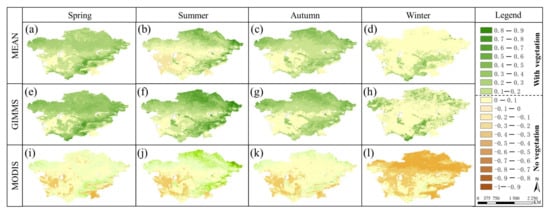
Figure 2.
Spatial distribution patterns of GIMMS NDVI (e–h), MODIS NDVI (i–l), and their mean values (a–d) in different seasons.
The NDVI in the growing season was calculated by using the monthly average NDVI from April to October. From 1981 to 1994, GIMMS NDVI showed a greening trend, with an annual increase rate of 0.0026. However, from 1994 to 2013, the greening trend lagged, with an annual increase rate of only 0.0001. During intersection time period, the value of GIMMS/MODIS NDVI (2000–2013) showed a browning trend. Furthermore, our results indicate that MODIS NDVI and GIMMS3g NDVI showed a significant positive correlation from 2000 to 2013 (correlation coefficient of 0.75, p < 0.01). The two sets of data have the same pattern of fluctuations and are found to have a slope of 0.983, R2 = 0.55 by the scatter plot. However, if we consider that the browning rate of MODIS NDVI is lower than that of the combined NDVI from 2000 to 2021, the reduction rate is only 0.00006 (Figure 3a).
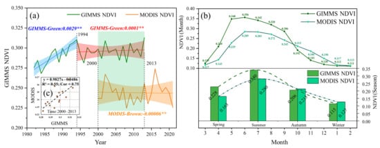
Figure 3.
Annual trends in GIMMS NDVI and MODIS NDVI, including their mean values and distribution of monthly (seasonal) NDVI within the year. (a) Annual NDVI trends, (b) annual and seasonal NDVI variations, (c) scatterplot of GIMMS NDVI and MODIS NDVI from 2000 to 2013. Note that ** indicates extreme significance (p < 0.01).
From the early 1980s to the mid-1990s, vegetation NDVI generally showed a greening trend. A relatively stable browning trend then emerged in the mid-1990s, with the decline from a high greening trend to a browning trend being relatively large. Meanwhile, when the annual changes of GIMMS NDVI and MODIS NDVI are examined further, both appear to be essentially the same, with a single peak change (from March), high values appearing in summer (June, July, and August), low values appearing in winter (December, January, and February), and a transition period appearing in spring and autumn (Figure 3b).
Additionally, GIMMS NDVI was higher in spring (0.225) than in autumn (0.206), and MODIS was higher in autumn than spring (0.215). Due to the inconsistency of the products, GIMMS NDVI is higher than MODIS NDVI in spring and summer (March–September) but lower in autumn and winter (October–February). In other words, the annual variation range of GIMMS NDVI is higher than that of MODIS NDVI, as shown in Figure 4b. The figure also shows that GIMMS NDVI is more sensitive to monthly (seasonal) changes in the year than MODIS NDVI, which may be reflected in the difference in the sensor’s band calculation (Figure 3b).
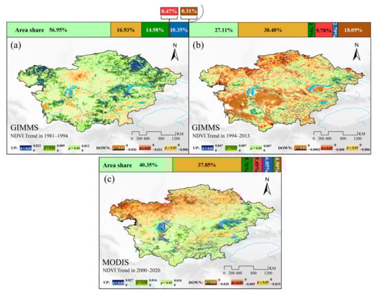
Figure 4.
Spatial variation trends for NDVI: (a,b) the GIMMS NDVI trends before and after 1994, respectively; (c) the MODIS NDVI trends from 2000 to 2020.
The results presented in Figure 4 show a spatially significant greening trend in GIMMS NDVI for the period 1981–1994, with an area share of 82.28%. The spatially highly significant (p < 0.01) greening trend of 0–0.022 was mainly pronounced in the northwest, northeast, and east–central mountain regions of Central Asia, with an area share of 10.35%. The spatially significant (0.01 < p < 0.05) greening trend of 0–0.009 was mostly concentrated around the highly significant rising area, with an area share of 14.98%. The spatially insignificant (p > 0.05) greening trend NDVI variation of 0–0.0012 was concentrated across the entire study region with an area share of 56.95%.
During 1981–1994, the spatial browning trend of NDVI was not obvious. It had an area share of only 17.72% and was mainly concentrated in the desert-steppe zone in the west–central region and the dry hot valley-basin zone in the southeastern mountains, such as the Ferghana Basin. The spatially significant (p < 0.01) browning trend NDVI variation was 0–0.026, accounting for only 0.31% of the area; the spatially significant (0.01 < p < 0.05) browning trend NDVI variation was 0–0.011, accounting for only 0.47% of the area; and the spatially significant (p < 0.05) browning area in total accounted for less than the spatially significant (p < 0.01) browning area (less than 0.8% of the total area) and was mainly concentrated around the Aral Sea Basin. The nonsignificant browning trend NDVI variation was 0–0.006, with 16.93% of the area covered (Figure 4a).
From 1994 to 2013, the GIMMS NDVI spatial browning trend was obvious, with an area share of 66.35%. Specifically, the spatially highly significant (p < 0.01) browning trend NDVI variation was 0–0.0002 and was mainly concentrated around the Aral Sea Basin, Lake Balkhash Basin, desert areas, and northern Kazakhstan, with an area share of 18.09%. Meanwhile, the spatially insignificant (p > 0.05) browning trend NDVI variation of 0–0.006 was mostly concentrated around the Central Asia, with an area of 34.48%. During this period, NDVI showed an insignificant spatial greening trend, with an area share of only 27.11%. The greening primarily occurred in the southwestern desert-steppe zone, Aral Sea Basin, Lake Balkhash Basin, and northeastern mountains. In this region, the spatially highly significant (p < 0.01) greening trend of NDVI varied from 0 to 0.047, with an area share of 2.79%, and the spatially significant (0.01 < p < 0.05) greening trend of NDVI varied from 0 to 0.007, with an area share of only 3.75%. Of note, spatially significant (p < 0.05) total area greening accounted for 6.54%, and the nonsignificant greening trend NDVI change was 0–0.007, covering 27.11% of the area (Figure 4b).
From 2000 to 2020, the MODIS NDVI spatial browning trend was obvious, with an area share of 47.84%. Specifically, the spatially highly significant (p < 0.01) browning trend NDVI variation was 0–0.020 and was mainly concentrated in Northwest Central Asia, with an area share of 4.50%. Meanwhile, the spatially insignificant (p > 0.05) browning trend NDVI variation of 0–0.015 was mostly concentrated around the northern region of 45° N in Central Asia, with an area of 37.85%. During this period, NDVI showed an insignificant spatial greening trend, with an area share of only 40.35%. The greening primarily occurred in the southwestern desert-steppe zone, Aral Sea Basin, Lake Balkhash Basin, and northeastern mountains. In this region, the spatially highly significant (p < 0.01) greening trend of NDVI varied from 0 to 0.027, with an area share of 6.05%, and the spatially significant (0.01 < p < 0.05) greening trend of NDVI varied from 0 to 0.016, with an area share of only 5.76%. Of note, spatially significant (p < 0.05) total area greening accounted for 11.81%, and the nonsignificant greening trend NDVI change was 0–0.016, covering 40.35% of the area (Figure 4c).
5.2. Factors Influencing NDVI Changes in Central Asia
To explore the influencing factors of NDVI changes in the study area, we first obtained the temporal and spatial distribution trends for VSP, VPD, and VAP. We found that the temporal and spatial variation trends for VSP and VPD were consistent from 1981 to 1994, and that both were negative. Furthermore, the spatial trend variation range for VSP was −0.12–0.08 hPa/year, the grid mean value was −0.05 hPa/year, and the average annual trend variation rate was −0.048 hPa/year. The spatial trend variation range for VPD was −0.29–0 hPa/year, the grid mean value was −0.06 hPa/year, and the average annual trend variation rate was −0.0060 hPa/year. Even though VAP displayed a positive trend, the spatial trend range was −0.05–0.24 hPa/year, the grid mean value was 0.01, and the average annual trend change rate was 0.012 hPa/year.
With regard to water vapor pressure, the climate environment from 1981 to 1994 exhibited a trend of wet and cold (Figure 5a,d,g). From 1994 to 2020, the temporal and spatial variation trends for VSP and VPD were consistent and positive. The spatial trend variation range of VSP was −0.07–0.11 hPa/year, the grid mean value was 0.03 hPa/year, and the average annual trend variation rate was 0.0030 hPa/year. Moreover, the spatial trend variation range for VPD was −0.01–0.12 hPa/year, the grid mean value was 0.03 hPa/year, and the average annual trend variation rate was 0.0034 hPa/year. VAP displayed a negative change trend, with the spatial trend range at −0.08–0.02 hPa/year, the grid mean value at 0, and the average annual trend change rate at −0.004 hPa/year. With regard to water vapor pressure, the climate environment from 1994 to 2020 indicated a trend of dry and hot. In general, the climate and environment of 1981–1994 (wet and cold) and 1994–2020 (dry and hot) showed an obvious opposite trend (Figure 5c,f,i).
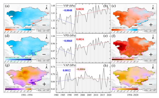
Figure 5.
Temporal and spatial variation trends for VSP, VPD, and VAP. For 1981–1994: (a) VSP, (d) VPD, and (g) VAP; for 1994–2020: (c) VSP, (f) VPD, and (i) VAP; for 1981–2020: Segmentation time trends in (b) VSP, (e) VPD, and (h) VAP before and after 1994, respectively.
Second, the temporal and spatial variation trends for PET, PRE, and SM were obtained. As can be seen, the temporal and spatial variation trends for PRE and SM were consistent and positive from 1981 to 1994. The spatial trend variation range for PRE was −10.85–23.31 mm/year, the grid mean value was 1.67 mm/year, and the average annual trend variation rate was −0.6667 mm/year. Meanwhile, the spatial trend variation range for SM was −24.47–38.89 mm/year, the grid mean value was 0.27 mm/year, and the average annual trend variation rate was 0.0224 mm/year. However, PET showed a negative change trend, with a spatial trend range of −12.45–2.96 mm/year, a grid mean value of −2.77, and an average annual trend change rate of −2.7663 mm/year.
Regarding water content, the climate environment from 1981 to 1994 indicated a clear trend of wet and cold (Figure 6a,d,g). From 1994 to 2020, the temporal and spatial variation trends of PRE and SM were consistent. Although they were positive (relatively negative), the degree trend was significantly lower than that of the previous stage. The spatial trend variation range of PRE was −3.44–4.94 mm/year, the grid mean value was 0.33 mm/year, and the average annual trend variation rate was 0.3256 mm/year, which is more than half lower than that in the previous stage. The spatial trend variation range of SM was −22.18–5.60 mm/year, the grid mean value was 0.08 mm/year, and the average annual trend variation rate was 0.0070 HPA/year. PET exhibited a positive trend, with a spatial trend range of −2.43–6.34 mm/year, a grid mean value of 2.09, and an average annual trend rate of 2.0855 mm/yr. In terms of water content, the climate environment from 1994 to 2020 charted a trend of dry and hot conditions. Overall, the climate environment showed a clear contradiction between 1981–1994 (wet and chilly) and 1994–2020 (dry and hot) (Figure 6c,f,i).
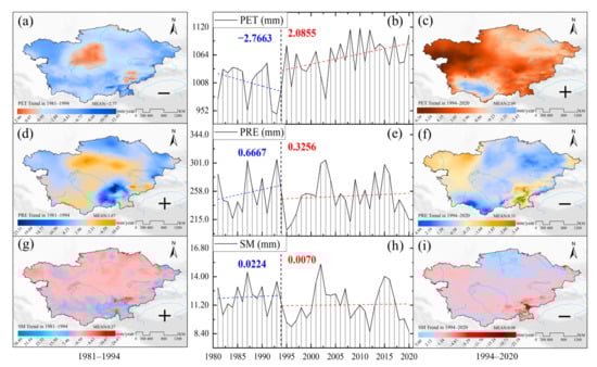
Figure 6.
Temporal and spatial trends of PET, PRE, and SM: 1981–1994: (a) PET, (d) PRE, and (g) SM; 1994–2020: (c) PET, (f) PRE, and (i) SM; for 1981–2020: Segmentation time trends in (b) PET, (e) PRE, and (h) SM before and after 1994, respectively.
By further exploring the correlation coefficient between environmental factors and NDVI, we found that NDVI was positively correlated with SM, PRE, and VAP, and negatively correlated with PET, VPD, and VSP. In terms of positive correlation, from 1981 to 1994 (GIMMS NDVI), NDVI had the highest positive correlation with PRE and the lowest positive correlation with SM (Figure 7a). However, from 1994 to 2013 (GIMMS NDVI) and 2000 to 2020 (MODIS NDVI), the positive correlation between NDVI and VAP was the highest, whereas the positive correlation with SM remained the lowest (Figure 7b,c). In terms of negative correlation, from 1981 to 1994, from 1994 to 2013, and from 2000 to 2020, NDVI had the highest negative correlation with VPD and the lowest negative correlation with VSP. To sum up, VPD with the highest negative correlation with NDVI and SM with the lowest positive correlation were selected for further investigations (Figure 7a–c).
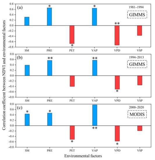
Figure 7.
Average annual correlation between environmental factors (SM, PRE, PET, VAP, VPD, and VSP) and NDVI: (a,b) average annual correlations about GIMMS NDVI before and after 1994, respectively; (c) average annual correlations about MODIS NDVI from 2000 to 2020. Note that * indicates significance (p < 0.05) and ** indicates extreme significance (p < 0.01).
Calculations of temperatures for the periods 1981–1994 and 1994–2020 show a decreasing trend with temperatures falling by approximately 0.05 °C per year in the former period and increasing by approximately 0.03 °C per year in the latter period (Figure 8a,b). Analysis of the temporal correlation with NDVI revealed a negative correlation between TEM and GIMMS NDVI in 1981–1994 (−0.148). From 1994–2013, the correlation between TEM and GIMMS NDVI was positive (0.218). In 2000–2020, the correlation between TEM and MODIS NDVI was positive (0.569). This further indicates that NDVI is browning with increasing temperature. The correlations between the above environmental factors and NDVI were all influenced by changes in temperature, and there is a pattern of consistency (correlations between TEM and the factors: SM: +; PRE: +; PET: −; VAP: −; VPD: +; VSP: +).
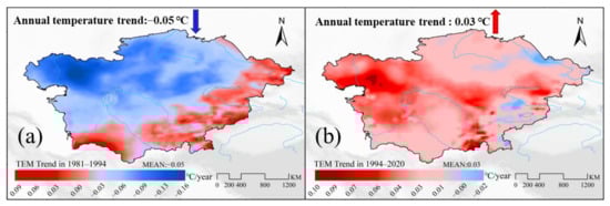
Figure 8.
(a,b) Temporal and spatial trends of temperature before and after 1994, respectively.
5.3. Dynamic Response of NDVI Changes to Drought in Central Asia
This paper further explores the impact of drought on NDVI and selects the Palmer Drought Severity Index (PDSI). The Palmer formula takes into account reference evapotranspiration, precipitation, surface moisture, and other indices, resulting in a more thorough response to meteorological drought. The PDSI possible values are as follows: 4.0 or higher (extremely wet), 3.0 to 3.99 (very wet), 2.0 to 2.99 (moderately wet), 1.0 to 1.99 (slightly wet), 0.5 to 0.99 (incipient wet spell), 0.49 to −0.49 (near normal), −0.5 to −0.99 (incipient dry spell), −1.0 to −1.99 (mild drought), −2.0 to −2.99 (moderate drought), −3.0 to −3.99 (severe drought), or −4.0 or lower (extreme drought) (Figure 9a).
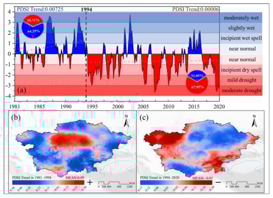
Figure 9.
Dynamic characteristics and temporal and spatial trends of PDSI in Central Asia: (a) monthly average dry and wet shade anomalies of PDSI from 1981 to 2020; (b,c) PDSI trends before and after 1994, respectively.
From 1981 to 1994, the monthly average rising trend of PDSI was 0.00725. The months above 0 (wet direction) accounted for 64.29%, and the months below 0 (dry direction) accounted for 35.71%. On the whole, Central Asia was developing a humid trend, with a grid average of 0.09. The humid trend (trend < 0) was concentrated in the peripheral areas of the region, accounting for 76.24% (Figure 9b).
From 1994 to 2020, the average monthly rising trend of PDSI was 0.0006, and the grid average was −0.01. The months above 0 (wet direction) accounted for 32.05%, and the months below 0 (dry direction) accounted for 67.95%, presenting the opposite time pattern to the previous stage. From these data, we can see that Central Asia was developing a drought trend.
The regions with a drought trend are distributed in the west and east of the study area, accounting for 51.42%, which is in the opposite spatial pattern from the previous stage. In general, the distribution of the wetting and drying trends in Central Asia in 1981–1994 and 1994–2020, respectively, indicates the objective law of the temporal and spatial consistency of humidity and drought, as well as the oppositional complementary trend in the order of magnitude of 1981–1994 (wet) and 1994–2020 (dry) (Figure 9c).
The study further explored the positive temporal and spatial correlation between GIMMS NDVI and PDSI. From 1981 to 1994, GIMMS NDVI and PDSI were positively correlated, with a grid mean of 0.38, of which 90.94% was in the positive correlation area and 9.06% in the negative correlation area (Figure 10a). From 1994 to 2013, GIMMS NDVI was positively correlated with PDSI. The grid mean was 0.29, with positive correlation areas accounting for 86.87% and negative correlation areas accounting for 13.13% (Figure 10b). During the period from 2000 to 2020, MODIS NDVI was positively correlated with PDSI. The grid mean was 0.33, with positive correlation areas accounting for 87.33% and negative correlation areas accounting for 12.67%. These results further explain the consistent rise and fall of NDVI with changes in drought degree under different products; that is, the lower the PDSI value (drought), the lower the NDVI value (Figure 10c).
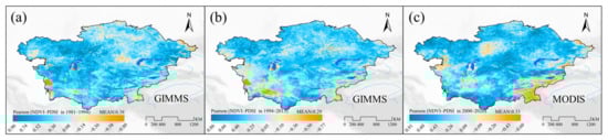
Figure 10.
Correlation between NDVI and PDSI in Central Asia: (a,b) correlations between GIMMS NDVI (1981–2013) and PDSI before and after 1994, respectively; (c) correlation between MODIS NDVI and PDSI from 2000 to 2020.
6. Discussion
According to the mechanism analysis of NDVI spatiotemporal changes in Figure 11, VPD and SM play a key role in vegetation growth. The transformation of vegetation from greening to browning is affected by many factors, such as changes in regional CO2 concentration, climate change (TEM, PRE, VPD, SM, PET, etc.), nitrogen deposition, and land-use change. If analyzed from a natural perspective, climate change is considered the main driving factor to explain vegetation greening [47,48,49]. The change in vegetation NDVI in Central Asia is greatly affected by climate factors. In this study, 1994 was the turning point of vegetation from greening to browning in Central Asia. We found, through the analysis of TEM, PRE, VPD, VAP, VSP, SM, and PDSI, that climate change before and after the turning point showed the opposite trend. Prior to the turning point, it was cold and wet, whereas after the turning point, it was hot and dry. Most studies show that low SM effectiveness and high VPD are considered the two main drivers of vegetation drought stress, which may pose a major threat to agricultural production and lead to extensive vegetation browning [50,51].
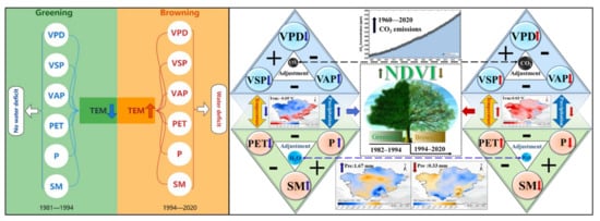
Figure 11.
Analytical diagram of NDVI spatiotemporal variation mechanism. The graph showing CO2 emissions presents the monthly mean carbon dioxide measured at the Mauna Loa Observatory, Hawaii, USA, from the Scripps Institution of Oceanography NOAA Global Monitoring Laboratory (https://gml.noaa.gov/ccgg/trends/mlo.html, accessed on 20 April 2022).
On the one hand, the change in vegetation NDVI is greatly affected by soil moisture conditions [51,52]. Studies have shown that the changes in NDVI from 1982 to 2015 are closely related to the changes in soil nutrient concentration and the availability of soil moisture [53,54] and that the temporal and spatial correlation between vegetation NDVI and soil moisture is significant. Moisture is the leading factor in vegetation change in East Africa [55]. In most study areas, especially in Central Asia, vegetation experiencing nonsignificant changes is limited by water [25].
On the other hand, the increase in CO2 concentration significantly promotes rises in temperature and leads to global warming [54]. Although climate warming will contribute to greening through photosynthesis, sustained warming will indirectly promote the failure of soil moisture use efficiency regulation by controlling the process of surface evapotranspiration and water consumption [56]. Finally, NDVI is reversed from greening to browning, which further indicates that the water shortage caused by drought will hinder the sustainable greening of vegetation, highlighting the negative ecological effect of climate warming [24,52,57].
Research clearly shows that since the early 1990s, the average temperature in Central Asia has increased substantially, potential and actual evapotranspiration has risen, average precipitation has decreased, and the frequency and intensity of extreme precipitation events have surged [58]. Additionally, since the early 1990s, soil water in Central Asia has shown a decreasing trend, and the climate water deficit has charted a steady upward trend [48]. These developments further aggravate the degree of drought. However, during the same time period (1994–2015), the actual water vapor pressure has shown a downward trend due to the reduction in ocean evaporation [59]. These factors have led to an increase in VPD just after the turning point mentioned in this study.
In a climate environment characterized by high VPD, vegetation stomata are closed, resulting in the deceleration or even failure of CO2 utilization efficiency. The outcome is vegetation carbon starvation [60]. At the same time, high VPD can lead to serious SM deficiency, which further worsens the health status of vegetation towards browning. In our research, we discovered that the increase in browning led to a slowdown in global average NDVI growth. Moreover, as drought may be the main reason for the increase in the browning trend, global vegetation growth may reverse from long-term greening to long-term browning if the future is warmer than average [31]. Overall, the combination of temperature rise and drought may be the main reasons for the transformation from greening to browning in Central Asia [37]. Although the browning trend has slowed down due to the influence of rising temperature and westerly precipitation, the browning continues as of 2020.
This paper conducted a comprehensive study on the independence and simultaneous establishment of two sets of NDVI products, which showed that the vegetation in Central Asia was greening before the turning point of 1994. After the turning point, the vegetation started to brown. The results of this study are notably important for the future health monitoring and management of vegetation ecosystems in Central Asia, which is of practical significance for regional ecological security assessment and sustainable development. In the future, more sets of products and site-measured data will be adopted to study vegetation NDVI changes, and more environmental factors will be added to conduct an in-depth study on vegetation NDVI changes, with the aim of making the driving mechanism of browning clearer.
7. Conclusions
From 1981 to 2020, the NDVI of different products in Central Asia showed a semicircular distribution pattern, with the Aral Sea Basin at the center and an upward trend from inside to outside. In terms of seasons, temporal changes clearly indicated that summer > spring > autumn > winter, and that GIMMS was more sensitive to yearly temporal changes than MODIS. During the study period, vegetation greening and browning initially coexisted until reaching a turning point in 1994, after which browning dominated. Vegetation in arid areas was shown to be more sensitive to water deficit caused by temperature changes in high VPD and low SM climate environments. At the same time, changes in vegetation NDVI were consistent with changes in drought degree, with lower PDSI values (the aggravation of drought degree) corresponding to vegetation browning. This study is of immense scientific value in its contribution to understanding the response of vegetation growth and carbon cycling to environmental changes and in its predictions of future developments in Central Asia.
Author Contributions
Conceptualization, J.X. and Y.C.; methodology, H.H.; data curation, H.H.; formal analysis, Y.L. and P.M.K.; writing—original draft preparation, H.H. and J.X.; writing—review and editing, H.H. and Z.L.; project administration, Y.C. and Z.L.; funding acquisition, Y.C. and Z.L. All authors have read and agreed to the published version of the manuscript.
Funding
This research is funded by the National Natural Science Foundation of China (Grant No. U2003302) and the Key Research Program of the Chinese Academy of Sciences (Grant No. U2003302ZDRWZS-2019-3).
Data Availability Statement
The data presented in this study are available on request from the corresponding author.
Conflicts of Interest
The authors declare no conflict of interest.
References
- Li, Y.; Chen, Y.; Sun, F.; Li, Z. Recent vegetation browning and its drivers on Tianshan Mountain, Central Asia. Ecol. Indic. 2021, 129, 107912. [Google Scholar] [CrossRef]
- Barbolini, N.; Woutersen, A.; Dupont-Nivet, G.; Silvestro, D.; Tardif, D.; Coster, P.; Meijer, N.; Chang, C.; Zhang, H.; Licht, A.; et al. Cenozoic evolution of the steppe-desert biome in Central Asia. Sci. Adv. 2020, 6, b8227. [Google Scholar] [CrossRef] [PubMed]
- Cavender-Bares, J.; Schneider, F.D.; Santos, M.J.A.O.; Armstrong, A.; Carnaval, A.; Dahlin, K.M.; Fatoyinbo, L.; Hurtt, G.C.; Schimel, D.; Townsend, P.A.; et al. Integrating remote sensing with ecology and evolution to advance biodiversity conservation. Nat. Ecol. Evol. 2022, 6, 506–519. [Google Scholar] [CrossRef]
- Liu, Y.; Li, Z.; Chen, Y.; Li, Y.; Li, H.; Xia, Q.; Kayumba, P.M. Evaluation of consistency among three NDVI products applied to High Mountain Asia in 2000–2015. Remote Sens. Environ. 2022, 269, 112821. [Google Scholar] [CrossRef]
- Gao, W.; Zheng, C.; Liu, X.; Lu, Y.; Chen, Y.; Wei, Y.; Ma, Y. NDVI-based vegetation dynamics and their responses to climate change and human activities from 1982 to 2020: A case study in the Mu Us Sandy Land, China. Ecol. Indic. 2022, 137, 108745. [Google Scholar] [CrossRef]
- Yang, W.; Zhao, Y.; Wang, Q.; Guan, B. Climate, CO2, and Anthropogenic Drivers of Accelerated Vegetation Greening in the Haihe River Basin. Remote Sens. 2022, 14, 268. [Google Scholar] [CrossRef]
- Rhif, M.; Abbes, A.B.; Martinez, B.; de Jong, R.; Sang, Y.; Farah, I.R. Detection of trend and seasonal changes in non-stationary remote sensing data: Case study of Tunisia vegetation dynamics. Ecol. Inform. 2022, 69, 101596. [Google Scholar] [CrossRef]
- Zhang, M.; Du, H.; Zhou, G.; Mao, F.; Li, X.; Zhou, L.; Zhu, D.E.; Xu, Y.; Huang, Z. Spatiotemporal Patterns and Driving Force of Urbanization and Its Impact on Urban Ecology. Remote Sens. 2022, 14, 1160. [Google Scholar] [CrossRef]
- Wang, J.; Han, P.; Zhang, Y.; Li, J.; Xu, L.; Shen, X.; Yang, Z.; Xu, S.; Li, G.; Chen, F. Analysis on ecological status and spatial–temporal variation of Tamarix chinensis forest based on spectral characteristics and remote sensing vegetation indices. Environ. Sci. Pollut. Res. 2022, 29, 5107–5123. [Google Scholar] [CrossRef]
- Piao, S.; Fang, J.; Zhou, L.; Zhu, B.; Tan, K.; Tao, S. Changes in vegetation net primary productivity from 1982 to 1999 in China. Glob. Biogeochem. Cycles 2005, 19, GB2027. [Google Scholar] [CrossRef] [Green Version]
- Zhou, L.; Tucker, C.J.; Kaufmann, R.K.; Slayback, D.; Shabanov, N.V.; Myneni, R.B. Variations in northern vegetation activity inferred from satellite data of vegetation index during 1981 to 1999. J. Geophys. Res. Atmos. 2001, 106, 20069–20083. [Google Scholar] [CrossRef]
- Rustanto, A.; Booij, M.J. Evaluation of MODIS-Landsat and AVHRR-Landsat NDVI data fusion using a single pair base reference image: A case study in a tropical upstream catchment on Java, Indonesia. Int. J. Digit. Earth 2022, 15, 164–197. [Google Scholar] [CrossRef]
- He, Y.; Oh, J.; Lee, E.; Kim, Y. Land Cover and Land Use Mapping of the East Asian Summer Monsoon Region from 1982 to 2015. Land 2022, 11, 391. [Google Scholar] [CrossRef]
- Zhang, Q.; Sun, C.; Chen, Y.; Chen, W.; Xiang, Y.; Li, J.; Liu, Y. Recent Oasis Dynamics and Ecological Security in the Tarim River Basin, Central Asia. Sustainability 2022, 14, 3372. [Google Scholar] [CrossRef]
- Li, Z.; Chen, Y.; Zhang, Q.; Li, Y. Spatial patterns of vegetation carbon sinks and sources under water constraint in Central Asia. J. Hydrol. 2020, 590, 125355. [Google Scholar] [CrossRef]
- Wang, C.; Liang, W.; Yan, J.; Jin, Z.; Zhang, W.; Li, X. Effects of vegetation restoration on local microclimate on the Loess Plateau. J. Geogr. Sci. 2022, 32, 291–316. [Google Scholar] [CrossRef]
- Liu, Y.; Li, Y.; Li, S.; Motesharrei, S. Spatial and temporal patterns of global NDVI trends: Correlations with climate and human factors. Remote Sens. 2015, 7, 13233–13250. [Google Scholar] [CrossRef] [Green Version]
- Karnieli, A.; Agam, N.; Pinker, R.T.; Anderson, M.; Imhoff, M.L.; Gutman, G.G.; Panov, N.; Goldberg, A. Use of NDVI and land surface temperature for drought assessment: Merits and limitations. J. Clim. 2010, 23, 618–633. [Google Scholar] [CrossRef]
- Mininni, A.N.; Tuzio, A.C.; Brugnoli, E.; Dichio, B.; Sofo, A. Carbon isotope discrimination and water use efficiency in interspecific Prunus hybrids subjected to drought stress. Plant Physiol. Biochem. 2022, 175, 33–43. [Google Scholar] [CrossRef]
- Ding, Y.; Xu, J.; Wang, X.; Peng, X.; Cai, H. Spatial and temporal effects of drought on Chinese vegetation under different coverage levels. Sci. Total Environ. 2020, 716, 137166. [Google Scholar] [CrossRef]
- West, E.; Morley, P.J.; Jump, A.S.; Donoghue, D. Satellite data track spatial and temporal declines in European beech forest canopy characteristics associated with intense drought events in the Rhön Biosphere Reserve, central Germany. Plant Biol. 2022. [Google Scholar] [CrossRef] [PubMed]
- Myneni, R.B.; Keeling, C.D.; Tucker, C.J.; Asrar, G.; Nemani, R.R. Increased plant growth in the northern high latitudes from 1981 to 1991. Nature 1997, 386, 698–702. [Google Scholar] [CrossRef]
- Kong, D.; Zhang, Q.; Singh, V.P.; Shi, P. Seasonal vegetation response to climate change in the Northern Hemisphere (1982–2013). Glob. Planet. Change 2017, 148, 1–8. [Google Scholar] [CrossRef] [Green Version]
- Pan, N.; Feng, X.; Fu, B.; Wang, S.; Ji, F.; Pan, S. Increasing global vegetation browning hidden in overall vegetation greening: Insights from time-varying trends. Remote Sens. Environ. 2018, 214, 59–72. [Google Scholar] [CrossRef]
- Xu, X.; Liu, H.; Jiao, F.; Gong, H.; Lin, Z. Time-varying trends of vegetation change and their driving forces during 1981–2016 along the silk road economic belt. Catena 2020, 195, 104796. [Google Scholar] [CrossRef]
- Zhong, L.; Hua, L.; Yao, Y.; Feng, J. Interdecadal aridity variations in Central Asia during 1950–2016 regulated by oceanic conditions under the background of global warming. Clim. Dynam. 2021, 56, 3665–3686. [Google Scholar] [CrossRef]
- Wang, X.; Chen, Y.; Li, Z.; Fang, G.; Wang, Y. Development and utilization of water resources and assessment of water security in Central Asia. Agric. Water Manag. 2020, 240, 106297. [Google Scholar] [CrossRef]
- Zhu, S.; Li, C.; Shao, H.; Ju, W.; Lv, N. The response of carbon stocks of drylands in Central Asia to changes of CO2 and climate during past 35 years. Sci. Total Environ. 2019, 687, 330–340. [Google Scholar] [CrossRef]
- Guan, X.; Yang, L.; Zhang, Y.; Li, J. Spatial distribution, temporal variation, and transport characteristics of atmospheric water vapor over Central Asia and the arid region of China. Glob. Planet. Chang. 2019, 172, 159–178. [Google Scholar] [CrossRef]
- Zhu, S.; Chen, X.; Zhang, C.; Fang, X.; Cao, L. Carbon variation of dry grasslands in Central Asia in response to climate controls and grazing appropriation. Environ. Sci. Pollut. Res. 2022, 29, 32205–32219. [Google Scholar] [CrossRef]
- Bandh, S.A.; Shafi, S.; Peerzada, M.; Rehman, T.; Bashir, S.; Wani, S.A.; Dar, R. Multidimensional analysis of global climate change: A review. Environ. Sci. Pollut. Res. 2021, 28, 24872–24888. [Google Scholar] [CrossRef] [PubMed]
- Martens, P. The political economy of water insecurity in Central Asia given the Belt and Road initiative. Cent. Asian J. Water Res. 2018, 4, 79–94. [Google Scholar] [CrossRef]
- Chen, Y.; Fang, G.; Hao, H.; Wang, X. Water use efficiency data from 2000 to 2019 in measuring progress towards SDGs in Central Asia. Big Earth Data 2022, 6, 90–102. [Google Scholar] [CrossRef]
- Yang, L.; Wei, W.; Wang, T.; Li, L. Temporal-spatial variations of vegetation cover and surface soil moisture in the growing season across the mountain-oasis-desert system in Xinjiang, China. Geocarto Int. 2021, 1–29. [Google Scholar] [CrossRef]
- Tai, X.; Epstein, H.E.; Li, B. Elevation and climate effects on vegetation greenness in an arid mountain-basin system of Central Asia. Remote Sens. 2020, 12, 1665. [Google Scholar] [CrossRef]
- Xuanli Liao, J. China’s energy diplomacy towards Central Asia and the implications on its “belt and road initiative”. Pac. Rev. 2021, 34, 490–522. [Google Scholar] [CrossRef]
- Fan, D.; Ni, L.; Jiang, X.; Fang, S.; Wu, H.; Zhang, X. Spatiotemporal analysis of vegetation changes along the belt and road initiative region from 1982 to 2015. IEEE Access 2020, 8, 122579–122588. [Google Scholar] [CrossRef]
- Pinzon, J.E.; Tucker, C.J. A non-stationary 1981–2012 AVHRR NDVI3g time series. Remote Sens. 2014, 6, 6929–6960. [Google Scholar] [CrossRef] [Green Version]
- Didan, K. MOD13Q1 V006: MODIS/Terra Vegetation Indices 16-Day L3 Global 250 m SIN Grid. NASA EOSDIS Land Processes DAAC. Available online: https://lpdaac.usgs.gov/products/mod13q1v006/ (accessed on 20 April 2022).
- Hersbach, H.; Bell, B.; Berrisford, P.; Hirahara, S.; Hor A Nyi, A.A.S.; Mu N Oz-Sabater, J.I.N.; Nicolas, J.; Peubey, C.; Radu, R.; Schepers, D.; et al. The ERA5 global reanalysis. Q. J. R. Meteorol. Soc. 2020, 146, 1999–2049. [Google Scholar] [CrossRef]
- Barbosa, S.; Scotto, M.G. Extreme heat events in the Iberia Peninsula from extreme value mixture modeling of ERA5-Land air temperature. Weather. Clim. Extrem. 2022, 36, 100448. [Google Scholar] [CrossRef]
- Kasten, F. Visibility forecast in the phase of pre-condensation. Tellus 1969, 21, 631–635. [Google Scholar] [CrossRef] [Green Version]
- Abatzoglou, J.T.; Dobrowski, S.Z.; Parks, S.A.; Hegewisch, K.C. TerraClimate, a high-resolution global dataset of monthly climate and climatic water balance from 1958–2015. Sci. Data 2018, 5, 170191. [Google Scholar] [CrossRef] [PubMed] [Green Version]
- Zhang, G.; Zhang, Y.; Dong, J.; Xiao, X. Green-up dates in the Tibetan Plateau have continuously advanced from 1982 to 2011. Proc. Natl. Acad. Sci. USA 2013, 110, 4309–4314. [Google Scholar] [CrossRef] [PubMed] [Green Version]
- Lee Rodgers, J.; Nicewander, W.A. Thirteen ways to look at the correlation coefficient. Am. Stat. 1988, 42, 59–66. [Google Scholar] [CrossRef]
- Stigler, S.M. Francis Galton’s account of the invention of correlation. Stat. Sci. 1989, 4, 73–79. [Google Scholar] [CrossRef]
- Chen, C.; Park, T.; Wang, X.; Piao, S.; Xu, B.; Chaturvedi, R.K.; Fuchs, R.; Brovkin, V.; Ciais, P.; Fensholt, R.; et al. China and India lead in greening of the world through land-use management. Nat. Sustain. 2019, 2, 122–129. [Google Scholar] [CrossRef]
- Lian, X.; Piao, S.; Chen, A.; Huntingford, C.; Fu, B.; Li, L.Z.; Huang, J.; Sheffield, J.; Berg, A.M.; Keenan, T.F.; et al. Multifaceted characteristics of dryland aridity changes in a warming world. Nat. Rev. Earth Environ. 2021, 2, 232–250. [Google Scholar] [CrossRef]
- Piao, S.; Wang, X.; Park, T.; Chen, C.; Lian, X.U.; He, Y.; Bjerke, J.W.; Chen, A.; Ciais, P.; T O Mmervik, H.; et al. Characteristics, drivers and feedbacks of global greening. Nat. Rev. Earth Environ. 2020, 1, 14–27. [Google Scholar] [CrossRef]
- Liu, L.; Gudmundsson, L.; Hauser, M.; Qin, D.; Li, S.; Seneviratne, S.I. Soil moisture dominates dryness stress on ecosystem production globally. Nat. Commun. 2020, 11, 4892. [Google Scholar] [CrossRef]
- Liu, L.; Teng, Y.; Wu, J.; Zhao, W.; Liu, S.; Shen, Q. Soil water deficit promotes the effect of atmospheric water deficit on solar-induced chlorophyll fluorescence. Sci. Total Environ. 2020, 720, 137408. [Google Scholar] [CrossRef]
- Wang, S.; Zhang, Y.; Ju, W.; Chen, J.M.; Ciais, P.; Cescatti, A.; Sardans, J.; Janssens, I.A.; Wu, M.; Berry, J.A.; et al. Recent global decline of CO2 fertilization effects on vegetation photosynthesis. Science 2020, 370, 1295–1300. [Google Scholar] [CrossRef] [PubMed]
- Willett, K.M.; Williams, C.N., Jr.; Dunn, R.; Thorne, P.W.; Bell, S.; De Podesta, M.; Jones, P.D.; Parker, D.E. HadISDH: An updateable land surface specific humidity product for climate monitoring. Clim. Past. 2013, 9, 657–677. [Google Scholar] [CrossRef] [Green Version]
- Cheng, L.; Zhang, L.; Wang, Y.; Canadell, J.G.; Chiew, F.H.; Beringer, J.; Li, L.; Miralles, D.G.; Piao, S.; Zhang, Y. Recent increases in terrestrial carbon uptake at little cost to the water cycle. Nat. Commun. 2017, 8, 110. [Google Scholar] [CrossRef] [PubMed] [Green Version]
- Wei, F.; Wang, S.; Fu, B.; Pan, N.; Feng, X.; Zhao, W.; Wang, C. Vegetation dynamic trends and the main drivers detected using the ensemble empirical mode decomposition method in East Africa. Land Degrad. Dev. 2018, 29, 2542–2553. [Google Scholar] [CrossRef]
- Ma, J.; Jia, X.; Zha, T.; Bourque, C.P.; Tian, Y.; Bai, Y.; Liu, P.; Yang, R.; Li, C.; Li, C.; et al. Ecosystem water use efficiency in a young plantation in Northern China and its relationship to drought. Agric. For. Meteorol. 2019, 275, 1–10. [Google Scholar] [CrossRef]
- Piao, S.; Nan, H.; Huntingford, C.; Ciais, P.; Friedlingstein, P.; Sitch, S.; Peng, S.; Ahlstr, O.M.A.; Canadell, J.G.; Cong, N.; et al. Evidence for a weakening relationship between interannual temperature variability and northern vegetation activity. Nat. Commun. 2014, 5, 5018. [Google Scholar] [CrossRef] [PubMed] [Green Version]
- Yao, J.; Chen, Y.; Chen, J.; Zhao, Y.; Tuoliewubieke, D.; Li, J.; Yang, L.; Mao, W. Intensification of extreme precipitation in arid Central Asia. J. Hydrol. 2021, 598, 125760. [Google Scholar] [CrossRef]
- Yu, L.; Weller, R.A. Objectively analyzed air–sea heat fluxes for the global ice-free oceans (1981–2005). Bull. Am. Meteorol. Soc. 2007, 88, 527–540. [Google Scholar] [CrossRef] [Green Version]
- Buermann, W.; Forkel, M.; O Sullivan, M.; Sitch, S.; Friedlingstein, P.; Haverd, V.; Jain, A.K.; Kato, E.; Kautz, M.; Lienert, S.; et al. Widespread seasonal compensation effects of spring warming on northern plant productivity. Nature 2018, 562, 110–114. [Google Scholar] [CrossRef] [Green Version]
Publisher’s Note: MDPI stays neutral with regard to jurisdictional claims in published maps and institutional affiliations. |
© 2022 by the authors. Licensee MDPI, Basel, Switzerland. This article is an open access article distributed under the terms and conditions of the Creative Commons Attribution (CC BY) license (https://creativecommons.org/licenses/by/4.0/).