1. Introduction
Over the last 30 years, with the rapid economic and social development in China [
1], drinking water sources have been heavily polluted by human activities [
2,
3]. Non-point source pollution (NPSP) is considered to be an important factor involved in the aforementioned problems in China [
4]. According to the results of the first national pollution survey [
5], more than half of the total nitrogen (TN) and total phosphorus (TP) discharged into the environment were produced by NPSP. The excessive input of nitrogen (N) and phosphorus (P) as a result of anthropogenic activities has caused water quality degradation in rivers [
6] and increased eutrophication [
7,
8]. Concurrently, the nutrient budget, meaning the surplus between input and export, retained in the watershed also pollutes the soil and aquifers [
9]. Therefore, it is vital to quantify the inputs and exports of anthropogenic N and P.
The input and export of N and P are two important components when quantifying nutrient budgets [
10]. The NPSP load entering the basin through leaching and runoff is subsequently exported into the river systems, which is known as the export of nutrients [
10]. N and P inputs strongly affect exports [
11]. The ratio of export to input is called the nutrient export ratio, and it reflects the capacity for nutrient retention and the potential risk of pollution in the riverine system [
12,
13]. Studies have shown that human activities can significantly affect the nutrient export ratio [
14]. For example, the N export ratio in the Taihu Lake Basin has increased from 18% to 30% in the last 30 years as a result of urbanization and population growth, and the N budget has changed accordingly [
13]. Hence, it is important to accurately and quantitatively estimate and predict the nutrient retention potential risk in riverine systems affected by human activities.
Model simulations are an important technical basis for the quantitative estimation and risk assessment of nutrients [
15]. Physical-based models, such as the Soil and Water Assessment Tool, can simulate the physical process of pollutants by using a large number of parameters [
16]. However, abundant parameters limit model application in data deficient areas [
17,
18]. The nutrient balance model is widely used in estimating N and P loads [
19]. The majority of studies integrate the Net Anthropogenic Nitrogen Input (NANI), the Net Anthropogenic Phosphorus Input (NAPI), and the Export Coefficient Model (ECM) methods to assess nutrient input and export, and their potential risks within the watershed system [
20]. For example, Lian et al. [
13] first integrated the NANI and ECM models to evaluate the N load at the county level in the Taihu Lake Basin and found that urbanization and population growth are the main factors disturbing the nitrogen budget. Deng et al. [
15] quantified the contribution rate of various factors to the NANI and NAPI models and constructed the management mechanism of nutrient diversity. These studies demonstrate that the nutrient balance model is a robust empirical model and is an effective predictor of N and P load [
13]. Moreover, the model can be easily used to assess nutrient variation in environmental systems, depending on whether their input variables (for example, N and P fertilization, atmospheric nitrogen fixation, crop nitrogen fixation) and export variables (domestic sewage, garbage, rural excrement, urban residents, livestock, and land use) are specific [
21]. However, the estimation of these nutrient balance variables is an imprecise process involving heavy calculations [
22]. For instance, nutrient balance models usually rely on statistical data and abundant estimation coefficients, and the differences in nutrient estimation coefficients have a certain impact on the model results [
13]. Secondly, statistical data are usually on the county level spatial scale, which poses a certain challenge in terms of accurately describing the spatial distribution of pollutants [
23].
Considering the aforementioned problems, machine learning models based on time series satellite images are regarded as a useful tool [
24,
25]. Firstly, machine learning models have a high simulation accuracy and fast training speed [
24]. This is important because it overcomes the problem whereby physical models are inadequate in data-deficient areas but also does not need to consider the influence of complex underlying surface characteristics on the estimated coefficients of the traditional model [
26,
27]. Secondly, remote sensing monitoring is an effective means to quantitatively evaluate pollutant exports and portray their spatial changes [
28] and is often used to identify and monitor NPSP exports [
20]. Human activities are the key factors affecting the input and export of nutrients [
12]. Therefore, a prediction model embedded with human activity indicators is necessary for estimating the input and export of nutrients.
The major objectives of this study were: (1) to build a nutrient prediction model embedded in human activity indicators to predict the input and export of nutrients; (2) to describe the spatial distribution of pollutant input and export; (3) to evaluate the potential risk of N and P retention in the watershed as a result of human activities.
3. Methods
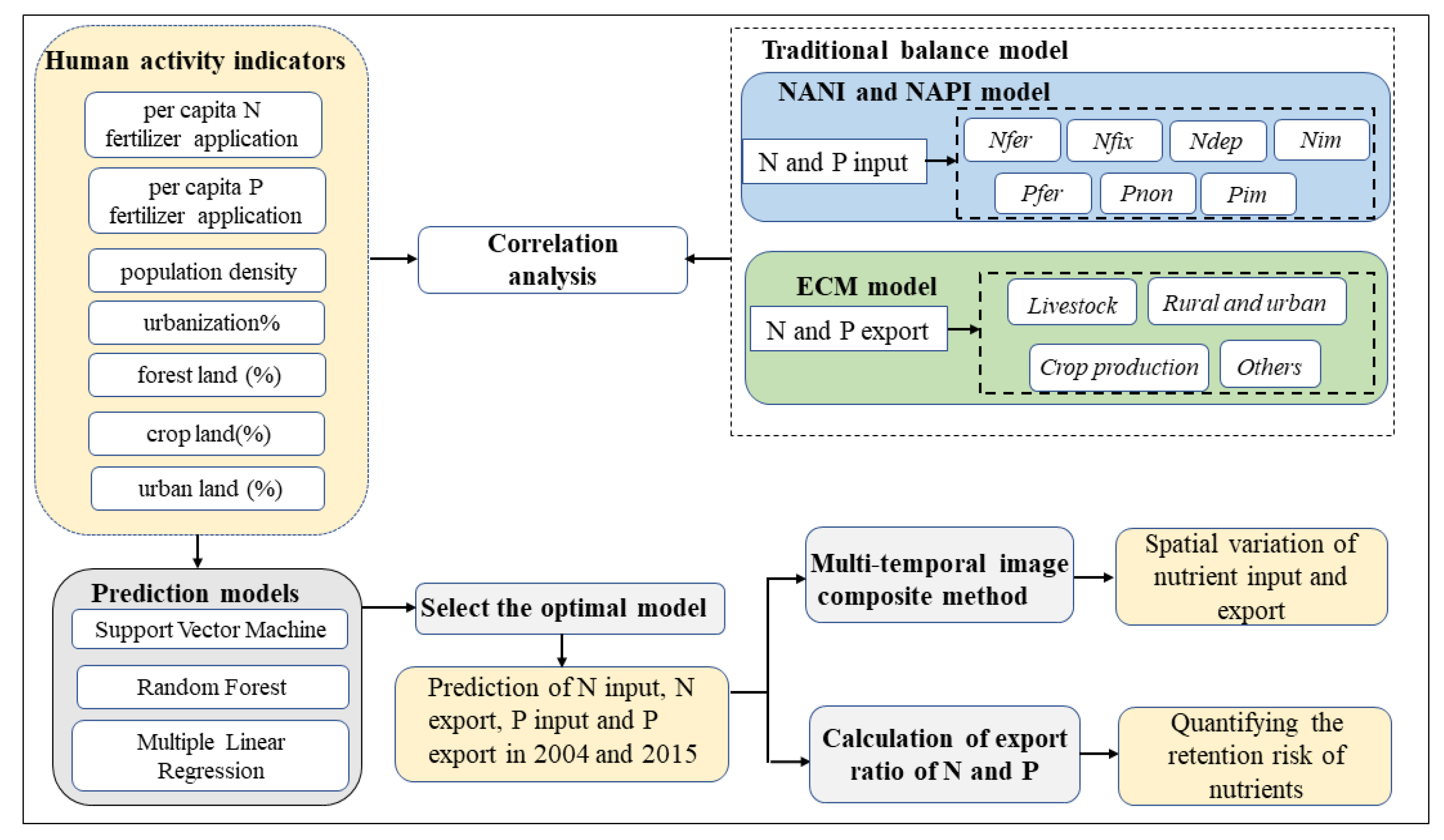
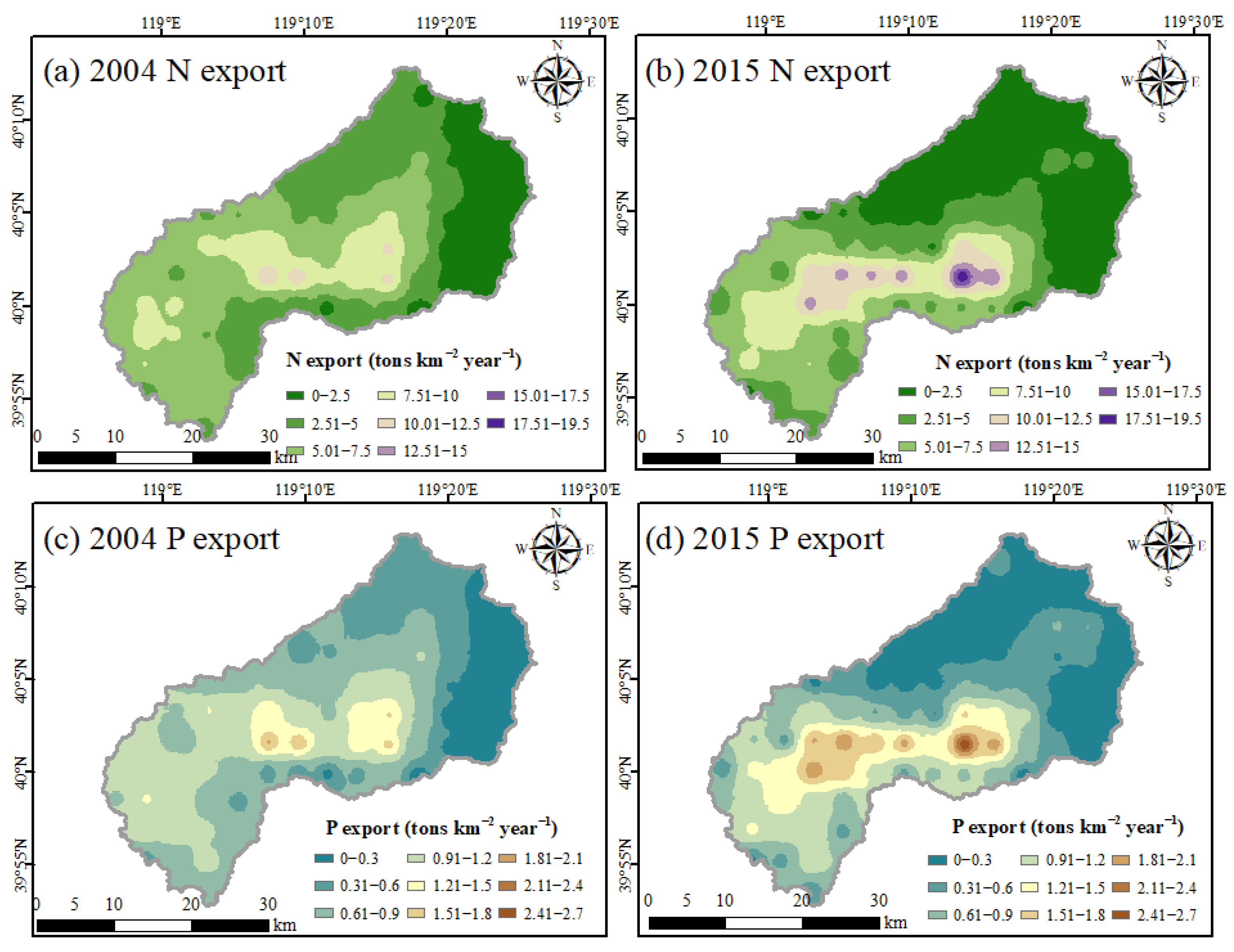
The overall objective was to build a convenient, reliable, and accurate annual-scale nutrient prediction model to predict nutrient input and export, and to assess the potential risk of nutrient retention in the watershed. The framework of this study is shown in
Figure 2. Firstly, we integrated traditional balance models, including the NANI, NAPI, and ECM models, and estimated the input and export of nutrients. Secondly, the Pearson correlation coefficient was used to select the human activity indicators that have an obvious impact on nutrient input and export, replacing the input variables of the traditional balance model. Subsequently, a nutrient prediction model based on the SVM, RF, and MLR algorithms was established, and the human activity indicators were used as the input data of the machine learning model to predict the input and export of nutrients. Thereafter, on the basis of Google Earth Engine (GEE), the area information of land-use types in the Yanghe Reservoir Basin was extracted using the multi-temporal fusion method and RF algorithm, and the spatial distribution of nutrient input and export was described. Finally, on the basis of the prediction results, we evaluated the potential risk of N and P retention in the watershed.
3.1. Preprocessing
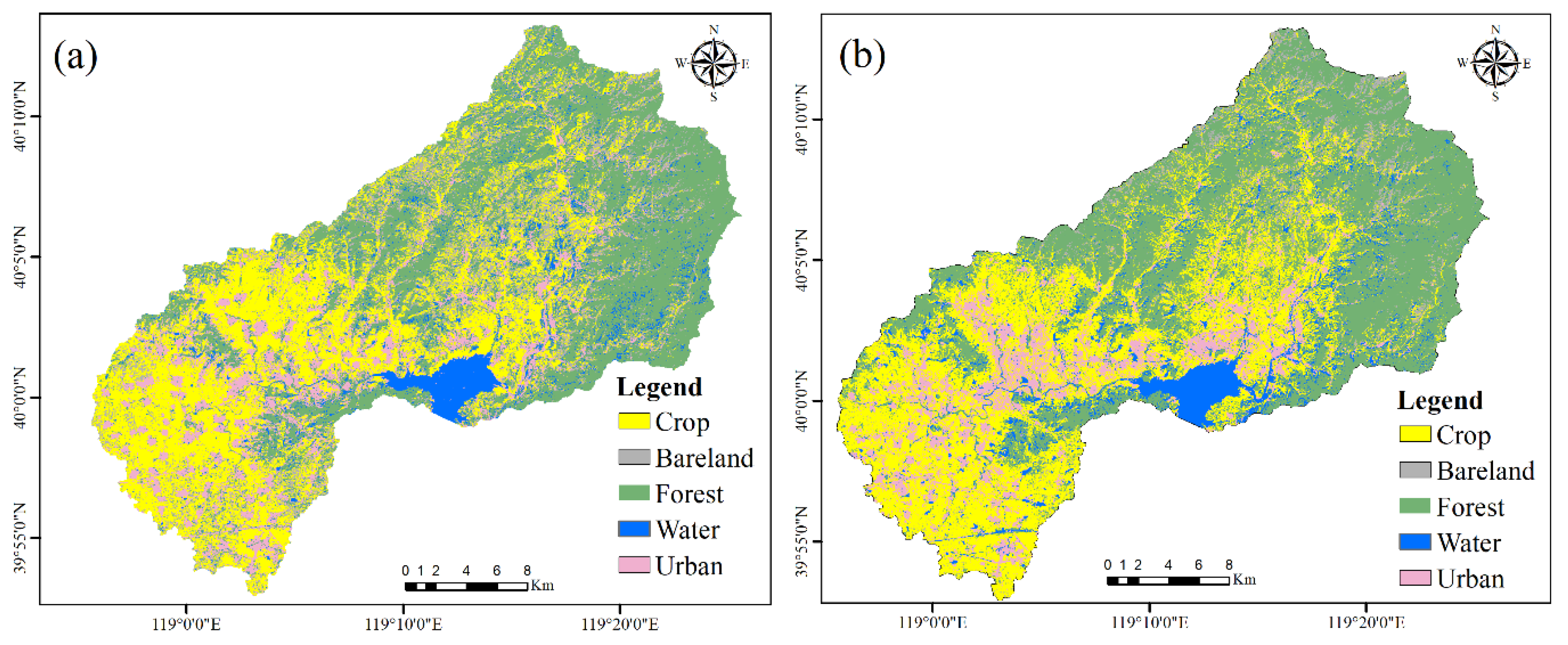
The land-use types have different ground features in different periods, which has a certain impact on the amount of N and P exported to the river outlet. We classified different land-use types in the study area from 2004 to 2015 for March to October based on the multi-temporal image fusion and RF classification algorithms (see the
Appendix A.1 and
Appendix A.2 for specific operations).
To describe the spatial distribution of pollutants, we converted the statistical data into human activity indicators on a spatial scale based on the area information of land-use types. Finally, the county-level statistical data were rasterized to a 3 km resolution for running the machine learning algorithm. The “create fishnet” tool in the data management tools, which is a part of ArcGIS desktop software version 10.4, was used for the spatial analysis of data. By drawing fishing nets, we were able to count the number of elements occupied by the grid and then analyze the spatial distribution characteristics of the data [
35,
36].
3.2. Nutrient Input and Export Estimation Based on the Traditional Balance Model
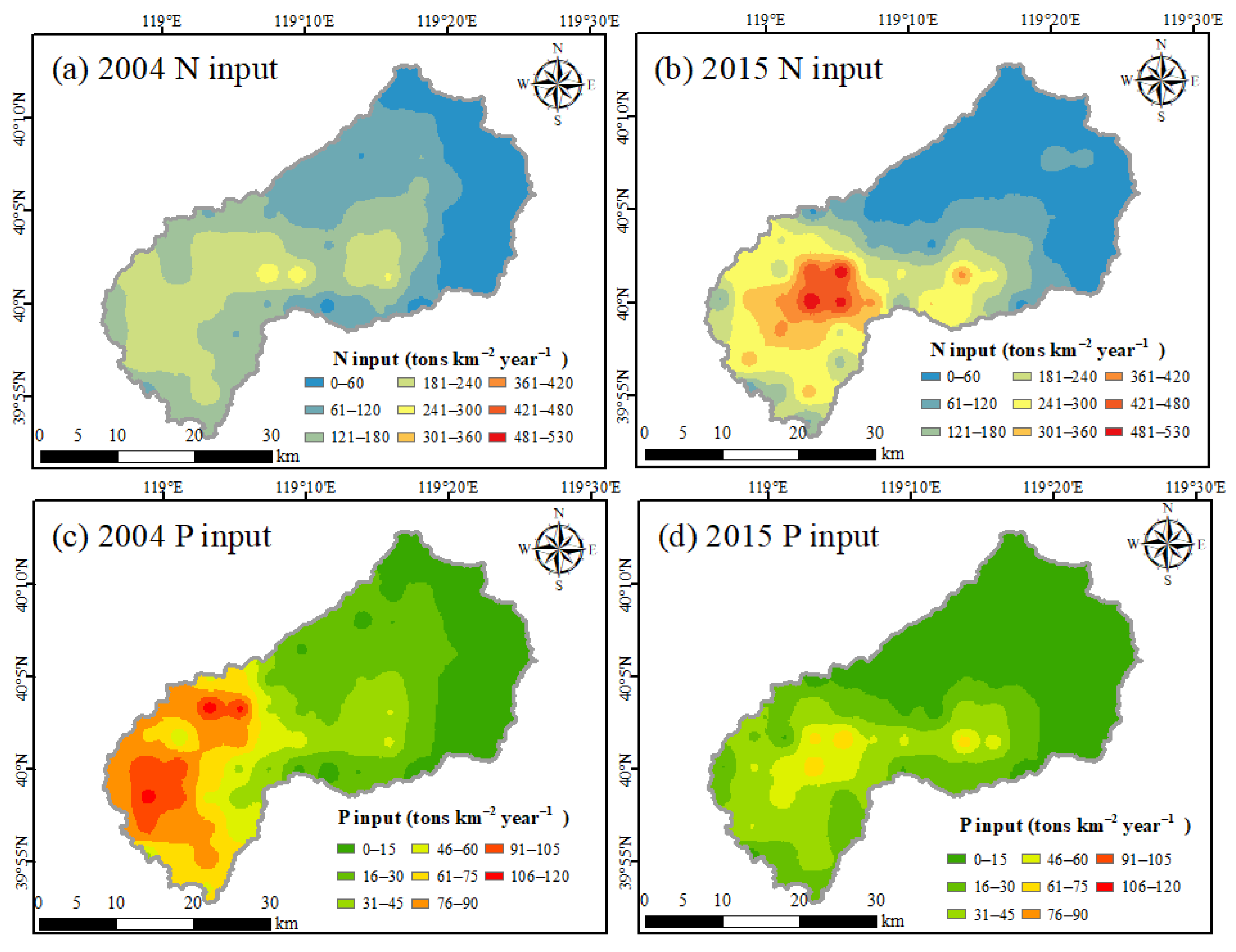
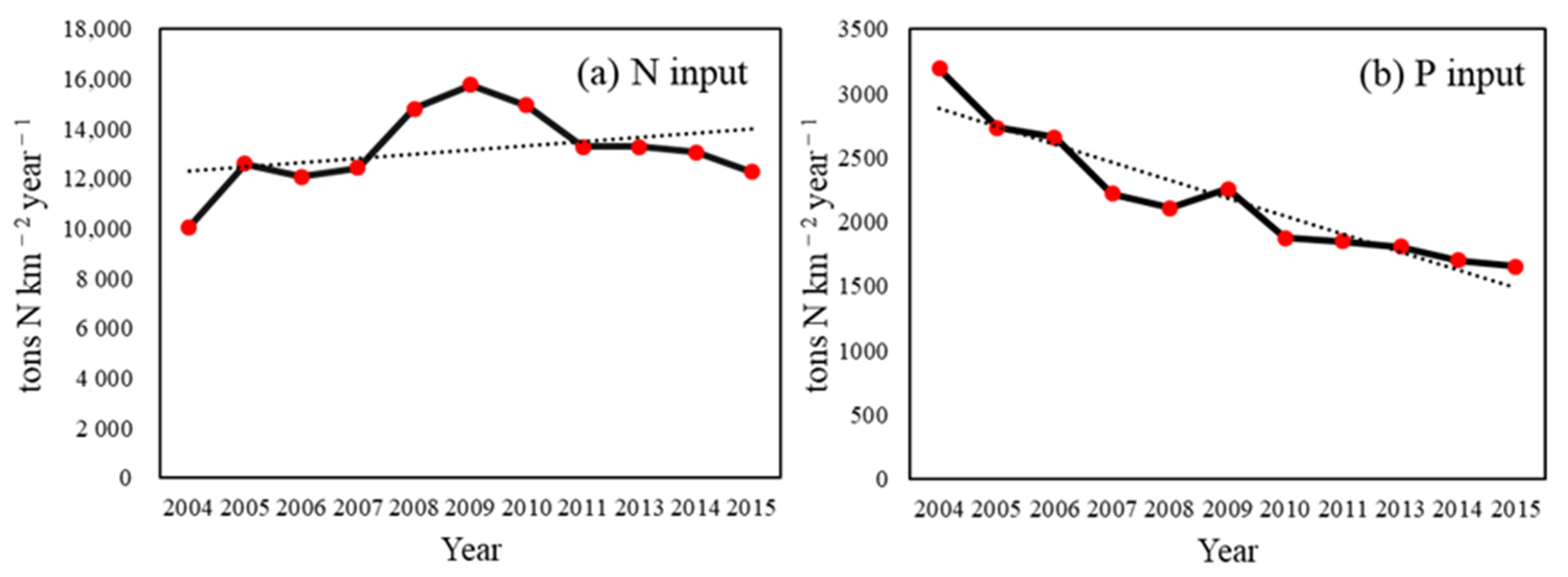
Traditional balance models, including the input model (NANI and NAPI), and the export model (ECM), were used to estimate the N and P input into the watershed and exported into the river, respectively. On the one hand, the results of the traditional model were used to select the human activity indicators that have a significant impact on nutrient input and export; on the other hand, they were used as validation data for the prediction model. The calculation process of NANI are represented in Equations (1) and (2):
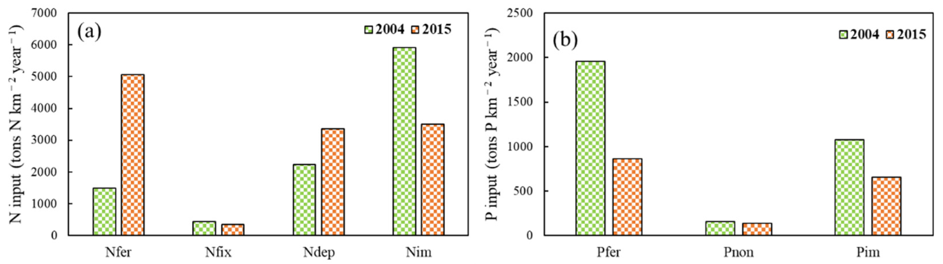
The NANI model is mostly composed of four trails, which include nitrogen fertilization (Nfer), atmospheric nitrogen deposition (Ndep), crop nitrogen fixation (Nfix), and net food/feed imports of Nitrogen (Nim). Nfer refers to the net fertilizer amount, which is the amount of nitrogen fertilizer converted according to 100% nitrogen. For the Ndep, only the oxidized nitrogen (NOx) was considered since the ammonium nitrogen (NHx) is not stable in the environment [
10]. Nfix mostly includes symbiotic nitrogen fixation and non-symbiotic nitrogen fixation. Both the peanuts and soybeans in the Yanghe Reservoir Basin are symbiotic nitrogen fixation crops. On the basis of previous studies [
37], the crop nitrogen fixation rate is shown in
Appendix A Table A6. Nim represents the net import of food and feed, wherein the net content means the surplus or deficit between N consumption and production. Nhum consumption and Nliv consumption denote the protein consumption in human food and livestock feed, respectively. Nliv products represent the N content of livestock products, which mainly refers to the meat, milk, eggs, and other livestock products. The nitrogen consumption and excretion level of each species are shown in
Appendix A Table A7. Ncro products represent the N content of agricultural crop production, which is shown in
Appendix A Table A8.
The NAPI model chiefly includes phosphorus fertilizer application (Pfer), non-food phosphorus input (Pnon), and net food/feed phosphorus imports (Pim). Among them, Pnon primarily comes from phosphorus detergent. We calculated the NAPI and Pim using Equations (3) and (4), as follows:
where Phum consumption and Pliv consumption represent human and livestock P consumption, respectively. Pliv products and Pcro products refer to the P content of livestock products and agricultural crop production, respectively. The calculation methods of Pfer and Pim are similar to that of NANI. The units of these variables are tons P km
−2 year
−1.
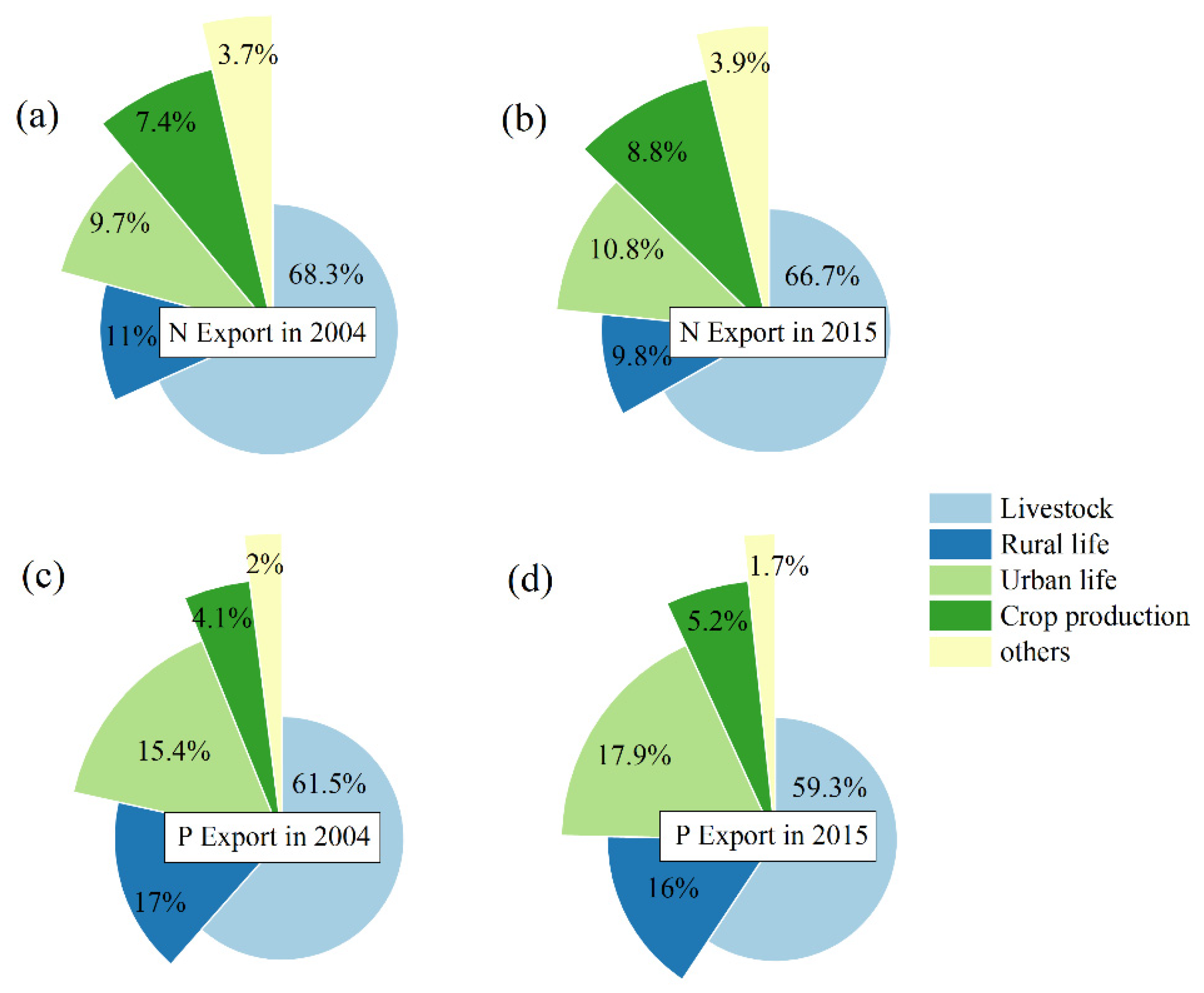
The ECM method is a mathematical weighted equation to estimate the N and P exports from different sources to the outlet of the Yanghe Reservoir Basin from 2004 to 2015. The main pollution sources included domestic sewage, garbage, and excrement from the rural region, urban residents, livestock, and land use (cropland, forest land, urban land, and bare land). This method is often used to express the relationship between pollutants (rural and urban areas), land use types, livestock, and N and P exports [
38,
39]. The formula of the ECM (Equation (5)) is as follows:
where
L represents the amount of nitrogen and phosphorus exports (t year
−1);
i is the type of pollution source;
j denotes the nutrient type, such as N and P;
Ei represents the annual export coefficient of each pollution source (kg km
−2 year
−1/kg ca
−1 year
−1) in
Table A9;
λij is the fraction of nutrient exports from the pollution source
i to the river outlet in
Appendix A Table A10;
Ai is the area of land use type (km
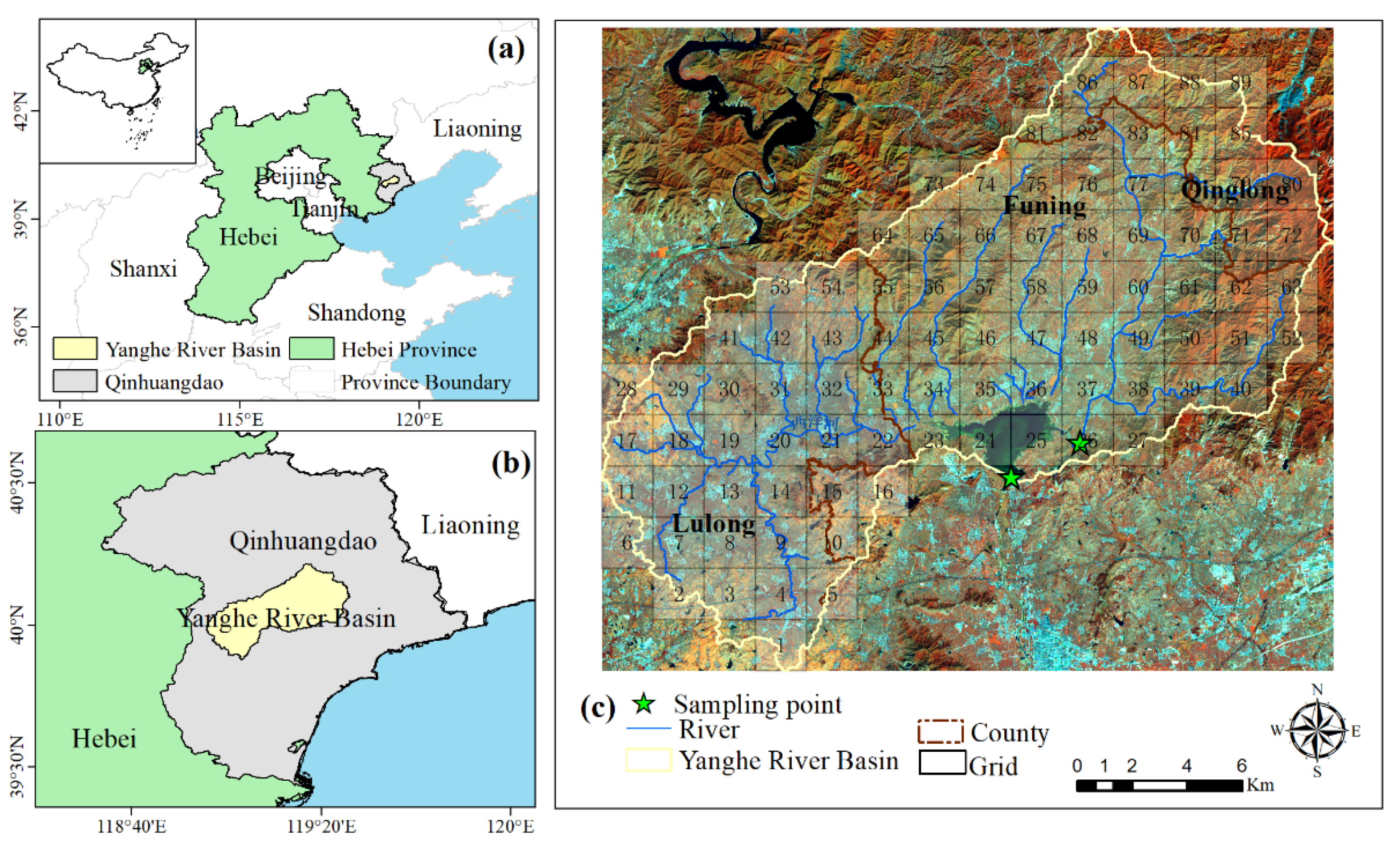
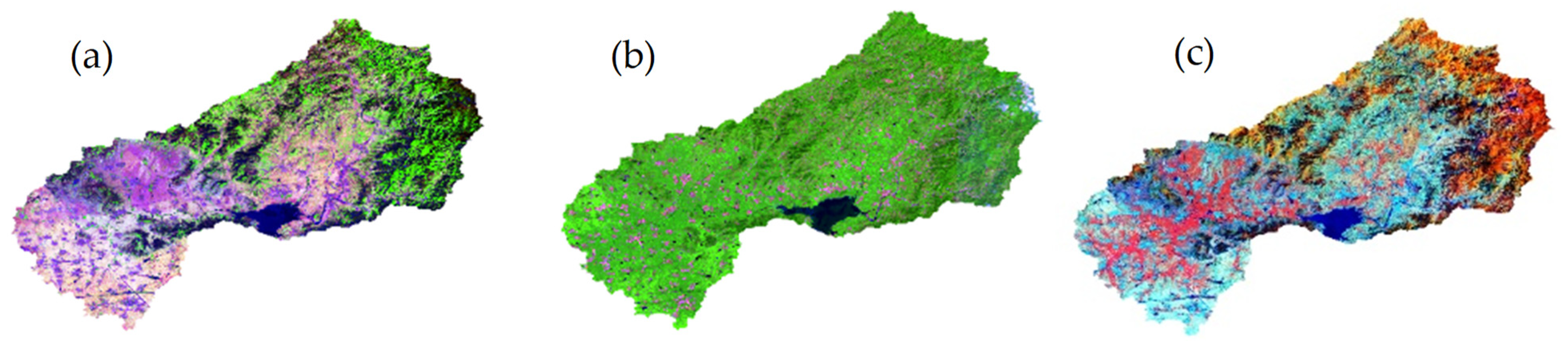
2) or the number of livestock (capita) and the population (people). The areas covered by the different land-use types from 2004 to 2015 were classified and extracted based on the multi-temporal fusion method and the RF classification algorithm. The livestock and population data of each county were derived from the local statistical yearbooks. We verified the results of the model with field monitoring data from May to October 2015. The sampling points are shown in
Figure 1c, and the results are shown in
Appendix A Table A11.
3.3. Prediction Model of Nutrient Input and Export
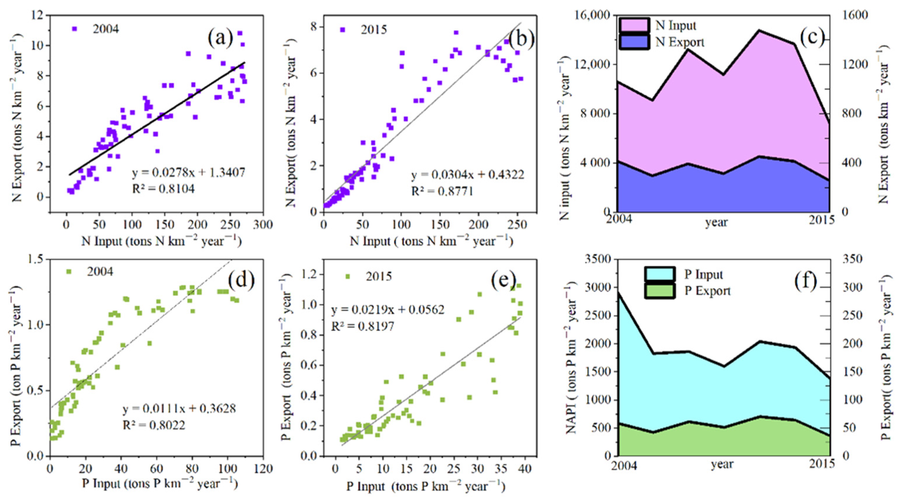
The primary purpose of machine learning model construction was to predict the N and P input into the watershed and exported into the river on an annual scale. Secondly, on the basis of the prediction results, the N and P export ratios were calculated. However, the rest of the export ratio represents the degree of potential pollution risk to soil and water quality caused by nutrient retention in the watershed.
To predict the input and export of N and P in 2004 and 2015, respectively, we set up 4 targets to obtain four predictor variables, as shown in
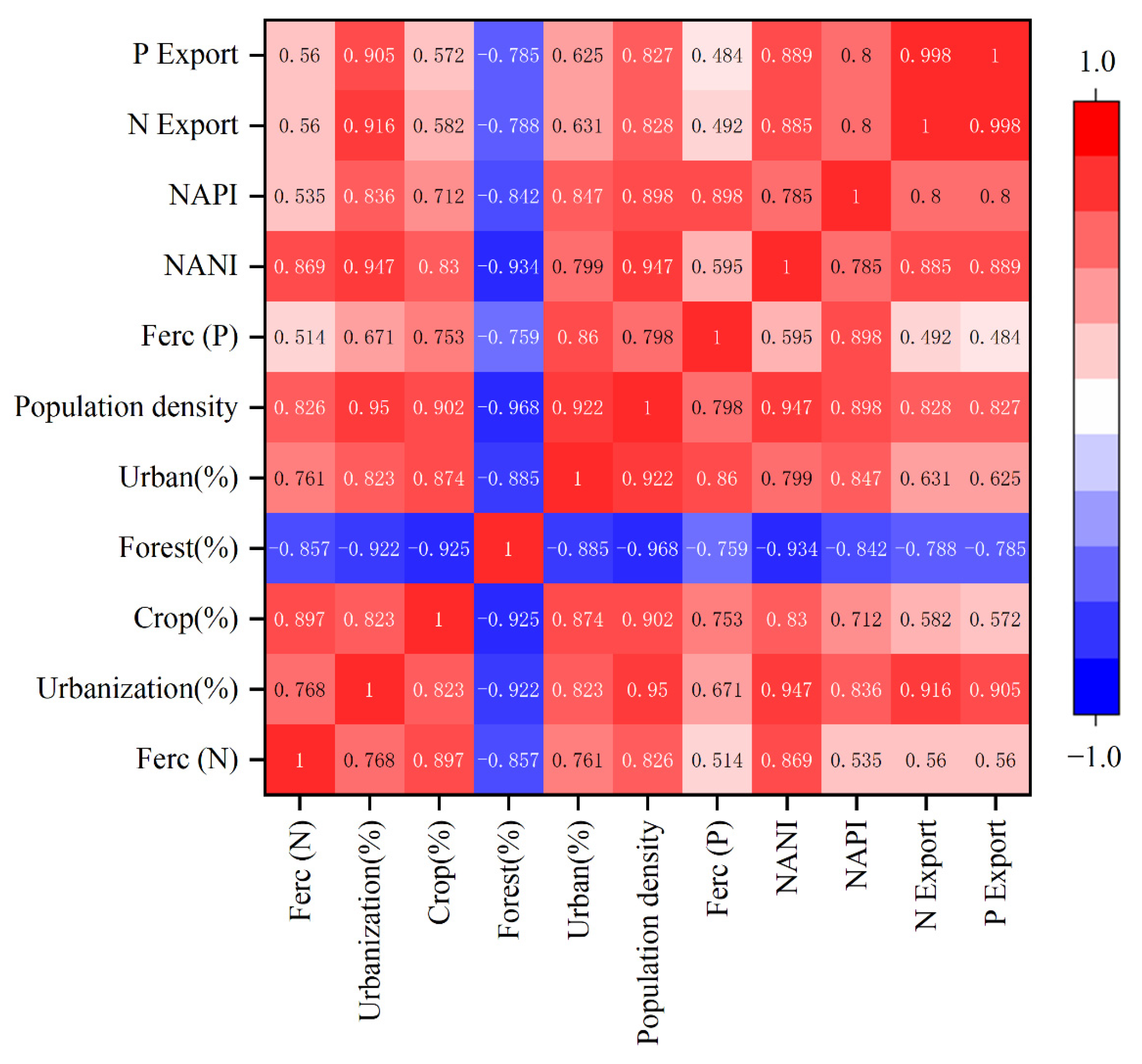
Table 3. On the basis of the estimation results of the traditional balance model, we used the Pearson correlation analysis to determine seven human activity indicators that have a significant impact on the input and export of N and P as the input data of the nutrient prediction model (See 4.1 for details). Those indexes include N and P fertilizer used per cultivated area (Ferc N and Ferc P (ton km
2)); the percentage of urban land area in the total area (urbanization (%)); the percentage of forest area (Forest (%)), crop area (Crop (%)) and urban area (Urban (%)) in each grid; and the population density (ca km
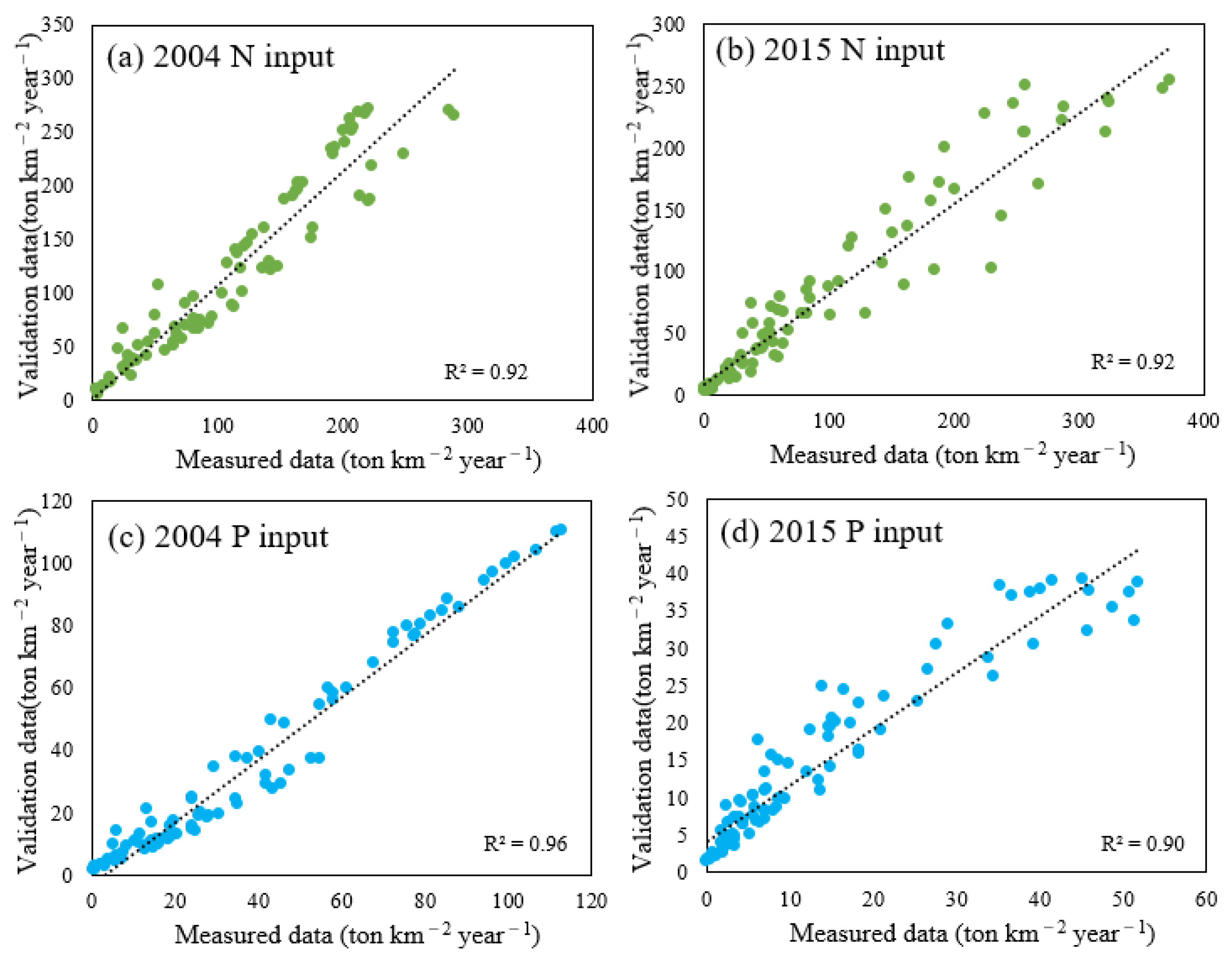
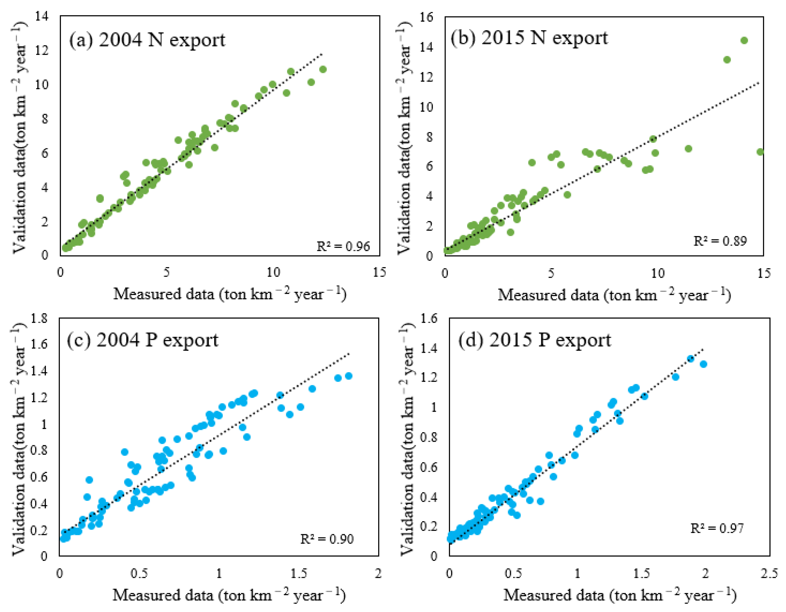
2), which is the average population per unit area of land. Before constructing the model, we performed pre-processing to remove autocorrelation, and transformed and unified the spatial scale of data, with a spatial resolution of 3 km. The time scale of model input data was 2004–2015. We determined the four variables predicted by the model, which are N and P inputs and exports. Thereafter, we divided the 980 sample points according into the training set and the testing at a ratio of 7:3. The SVM, RF, and MLR models were selected to construct the nutrient prediction model. As compared with the traditional model, machine learning can identify an optimal segmentation point, which can tackle both linear and nonlinear relationships. However, the traditional model can-not directly tackle non-linearity. When training the model, we configured and adjusted the super parameters to obtain the best performance, we determined the iterative method from the best super parameters, and we set the number of iterations to 100. Tenfold cross-validation was used to test the accuracy of the algorithm. The determination coefficient (R
2) and RMSE was used to evaluate the results of the prediction model and the optimal model was selected based on this.
3.3.1. Support Vector Machine (SVM)
SVM is a supervised learning algorithm that is mainly based on the principle of structural risk minimization and statistical learning theory [
39]. To achieve the purpose of accurate classification of various types of data, the interval maximization method was used to find the maximum classification interval of the defined feature space in the data [
40]. Moreover, in order to reduce the impact resulting from the limited sample data, the hyperplane analysis method was used to distance the sample data from this hyperplane [
41]. When nonlinear problems are encountered, the kernel function can be used for mapping analysis [
41,
42]. The algorithm identifies the optimal parameter combination using the gradient descent method. The number of optimization iterations set by the program was 100. We used the sigmoid kernel function with hyperparametric penalty coefficient c, which improved the generalization ability of the model, with a value of 1. The values of hyperparameters gamma and coef0 were 0.7 and 0.4, respectively [
36,
43].
3.3.2. Random Forest (RF)
In this study, RF was used not only for land-use classification, but also for the N and P input and export predictions. The RF method is an extension of the bagged classification tree considering the ensemble learning theory, which can improve the accuracy of models [
4,
44]. RF is an integrated model that uses a set of independent classification or regression trees to achieve classification or regression aims [
36]. The advantage of the RF algorithm is that it is not sensitive to the noise in the training set, and is more conducive to obtaining a robust model and avoiding overfitting conditions [
45]. The randomness of RF is reflected in two aspects. The first is the randomness of samples [
46]: a certain number of samples are randomly selected from the training set as the root node samples of each regression tree. The second is the randomness of features: when establishing each regression tree, a certain number of candidate features are randomly selected, and the most appropriate feature is selected as the splitting node. During parameter adjustment, the value of the max_depth of the decision tree was 10. When the depth of the tree reaches the maximum depth, the decision tree will stop operation no matter how many features can be branched. The n_estimators denote the number of decision trees, and the value is 2000. The max_features is one of the super parameters, which was set to 3. The maximum percentage of features considered in the decision tree was 10%. The selection of parameter values was conducted according to previous research [
44,
45,
46].
3.3.3. Multiple Linear Regression (MLR)
Multiple linear regression is a widely used linear regression method [
46]. A phenomenon is often associated with multiple factors, for example it is more effective and practical to predict or estimate dependent variables using the optimal combination of multiple independent variables than to predict or estimate only one independent variable [
47]. To measure the error between the estimated value and the real value, a non-negative real number function is usually selected as the loss function in the linear regression model. The smaller the value of the non-negative real loss function, the smaller the error. The least-squares method is generally applicable to parameters estimation [
48]. We used the MLR model to represent the relationship between the nutrient inputs, exports, and human indicators, and to explore the change characteristics of nutrients as a result of intensive human activities.
6. Conclusions
In this study, we built a convenient, reliable, and accurate nutrient prediction model for estimating nutrient input and export and evaluating the potential nutrient retention risk for drinking water sources. The prediction model reduced the uncertainty caused by the traditional nutrient balance estimation methods, which rely on statistical data and a large number of estimation coefficients. Remote sensing images and the multi-temporal fusion method were used to select sample points, and the RF algorithm was incorporated to identify the pollution sources such as forest land, bare land, cropland, water, and urban land in the drinking water sources area. The overall classification low-end accuracy was 92%. The performance of the prediction model based on SVM was better than those based on RF and MLR. The results of the prediction model were of the same order of magnitude as those of traditional N and P estimation methods and demonstrated that the nutrient prediction model is reliable. The export ratios of N and P under human disturbance were 2.8–3.0% and 1.1–2.2%, respectively. The excessive N and P (97% to 98%) in the riverine system pose a potential risk to the drinking water sources. Next, we will introduce climate change factors, including rainfall, into our nutrient prediction model in order to assess the potential risks of the combined impact of human activities and climate change on nutrient retention.


 and
and 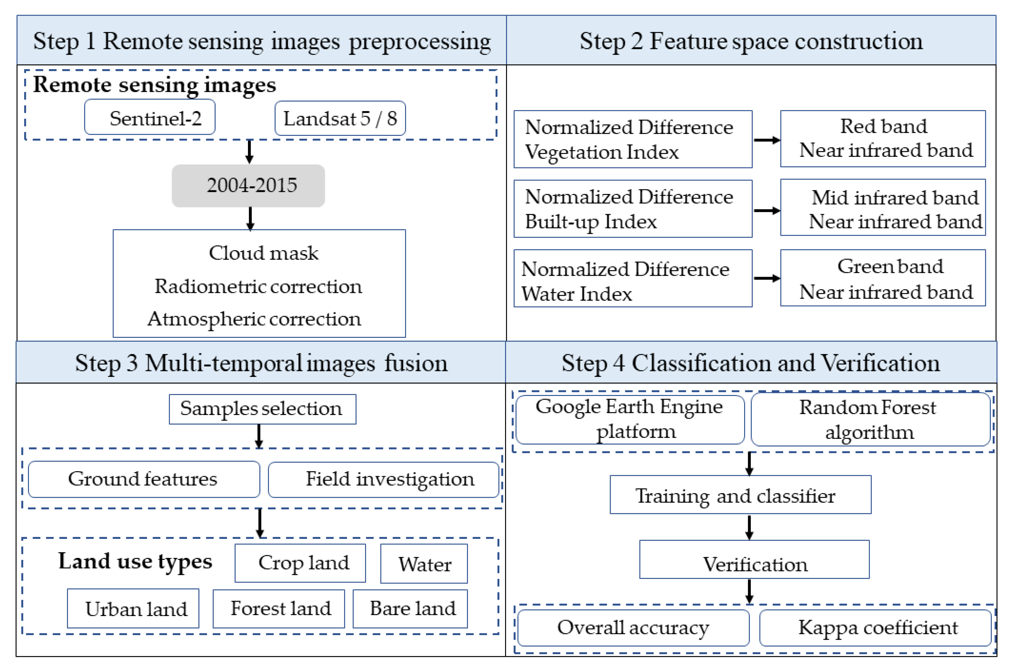
