Shipborne GNSS-Determined Sea Surface Heights Using Geoid Model and Realistic Dynamic Topography

Abstract

With an increasing demand for accurate and reliable estimates of sea surface heights (SSH) from coastal and marine applications, approaches based on GNSS positioning have become favored, to bridge the gap between tide gauge (TG) and altimetry measurements in the coastal zone, and to complement offshore altimetry data. This study developed a complete methodology for jointly deriving and validating shipborne GNSS-determined SSH, using a geoid model and realistic dynamic topography estimates. An approach that combines the properties of hydrodynamic models and TG data was developed to obtain the latter. Tide gauge data allow estimating the spatiotemporal bias of a hydrodynamic model and, thus, linking it to the used vertical datums (e.g., a novel geoid-based Baltic Sea Chart Datum 2000). However, TG data may be erroneous and represent different conditions than offshore locations. The qualities of spatiotemporal bias are, hence, used to constrain TG data errors. Furthermore, a rigid system of four GNSS antennas was used to ensure SSH accuracy. Besides eliminating the vessel’s attitude effect on measurement data, the rigid system also provides a means for internal validation, suggesting a 4.1 cm height determination accuracy in terms of standard deviation. The methodology also involves eliminating the effect of sea state conditions via a low-pass filter and empirical estimation of vessel sailing-related corrections, such as the squat effect. The different data validation (e.g., examination of residual values and intersection analyses) results, ranging from 1.8 cm to 5.5 cm in terms of standard deviation, indicate an SSH determination accuracy of around 5 cm.

1. Introduction

Sea surface height (SSH), an imperative parameter for understanding the marine environment, sees an increasing demand for accurate and reliable estimates from coastal and marine applications (e.g., engineering, navigation, research). Historically, tide gauge (TG) stations, some as old as a few centuries, have provided continuous sea level information, which is now essential, for instance, to climate studies [1,2,3]. Although modern TGs also allow a high accuracy (centimeter-level) and sampling rate (up to seconds), the distribution of TG stations is generally sparse and restricted to land-bound coastal locations. Since the TG-determined sea level information represents only a limited spatial domain, complementary data from space geodetic techniques are invaluable. Satellite altimetry (SA) records now span over three decades, densely covering most of the Earth’s marine areas with a reasonable quantification of SSH [4,5,6]. However, the SA method is often limited by its spatial and temporal resolution characteristics and reliability, which tend to diminish in the coastal zone due to approximations in atmospheric, sea state, and geophysical corrections and waveform distortions caused by coastal inhomogeneities [7,8,9].

Approaches based on GNSS (global navigation satellite system) positioning have, thus, become favored for bridging the gap between TG and SA measurements in the coastal zone and complementing SA data offshore. These methods are also appropriate for the validation and calibration of SA-based SSH, in addition to commonly used TG-based methods. It has been demonstrated that relatively accurate SSH can be acquired by shipborne GNSS measurements [10,11,12], airborne laser scanning surveys [13,14,15], and other alternatives, such as GNSS-equipped buoys [16,17] and uncrewed sea vessels [18,19]. While airborne laser scanning surveys currently require expensive equipment and a survey aircraft, and buoys or uncrewed vessels may first demand watercraft development, the shipborne GNSS approach appears most convenient. Some studies have used transit vessels (e.g., ferries) and their routes for research purposes [20,21,22], demonstrating that dedicated survey vessels and routes are not necessarily required either.

In the spring and summer of 2021, six marine survey campaigns were conducted with the primary focus on marine condition monitoring of the Baltic Sea. Concurrently, four GNSS devices installed on the research vessel collected SSH data autonomously. In [23] are provided a comprehensive review of the six marine survey campaigns, discussions concerning the problems occurring during autonomous data collection, and a description of the GNSS data post-processing. Following lessons learned in our previous studies [11,24], this paper presents improved data processing approaches and a complete exploration of the methodology for deriving accurate SSH from initial post-processed GNSS measurements (i.e., instantaneous SSH), which, unless further treated, are impractical for use in data applications. Accurate derivation of shipborne GNSS-based SSH requires consideration of a vessel’s high-frequency attitude changes (e.g., pitch and roll motions) [11] and sea state conditions (i.e., waves) [24], which contaminate the instantaneous SSH, but also need vessel sailing-related corrections [11]. These corrections account for the squat effect, which causes a moving vessel to sail deeper than its nominal draft, and gradual changes in the static draft (e.g., continuous fuel consumption causes a vessel to float higher).

Aside from deriving SSH, the developed methodology involves a joint validation of the results, demanding comparable data from an independent source. It will be demonstrated that such a joint approach can enhance data accuracy by processing residual values instead of the instantaneous SSH. Thus, the emphasis of the study is also on the structuring of validation datasets. Since SSH is the sum of geoidal height and dynamic topography (DT), a suitable geoid model and DT estimates are required. In the current study, an essential component of the latter is the recently initiated implementation of the Baltic Sea Chart Datum 2000 (BSCD2000), a common height reference for the Baltic Sea region [25,26]. The BSCD2000 will be realized through GNSS and geoid modeling (i.e., BSCD2000 is an equipotential surface) and is compatible with the EVRS (European Vertical Reference System) associated national height system realizations of the Baltic Sea countries. As the Baltic Sea TGs are rigorously connected to the national height systems [27,28], the TG readings refer to the BSCD2000 at the reference epoch, implying that the contemporary TG readings can be expressed directly as DT (cf. Figure 1).

However, because TG stations are generally distributed in sparse land-bound coastal locations, hydrodynamic models (HDMs) providing high spatial and temporal (hourly) resolution DT may appear an appealing offshore data source. Caution should be exercised using these models, since they usually contain a long-wavelength nature [29,30] spatiotemporal dynamic bias (DB) relative to the used height reference [15,30,31] (also refer to Figure 1). Hence, it would be advantageous to employ the method developed by [15,30]: the DB estimated at TG stations is gridded and then removed from an HDM; therefore, linking the model with height references. In these studies, exact interpolators were employed for gridding. Such an approach assumes that a DB estimate at a TG station is errorless and represents all nearby offshore locations, which may not be necessarily true. Utilizing the qualities of DB, an approach was developed for estimating DB uncertainties used during offshore DB prediction by least-squares collocation (i.e., an inexact interpolator); thus, constraining TG data errors. By combining the properties of TG data and HDMs, realistic DT can be derived for shipborne GNSS-determined SSH validation.

This contributions’ outline is as follows. Section 2 reviews the core theoretical principles for deriving and validating shipborne GNSS-determined sea surface heights (note that subsequent sections reveal additional details with data examples, since these reinforce the developed principles). Section 3 provides an overview of the shipborne GNSS surveys and used information. The derivation of offshore DT is examined next in Section 4; whereas, Section 5 is dedicated to shipborne GNSS data processing and validation. The paper continues with a discussion in Section 6 and concludes with a summary in Section 7.

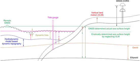
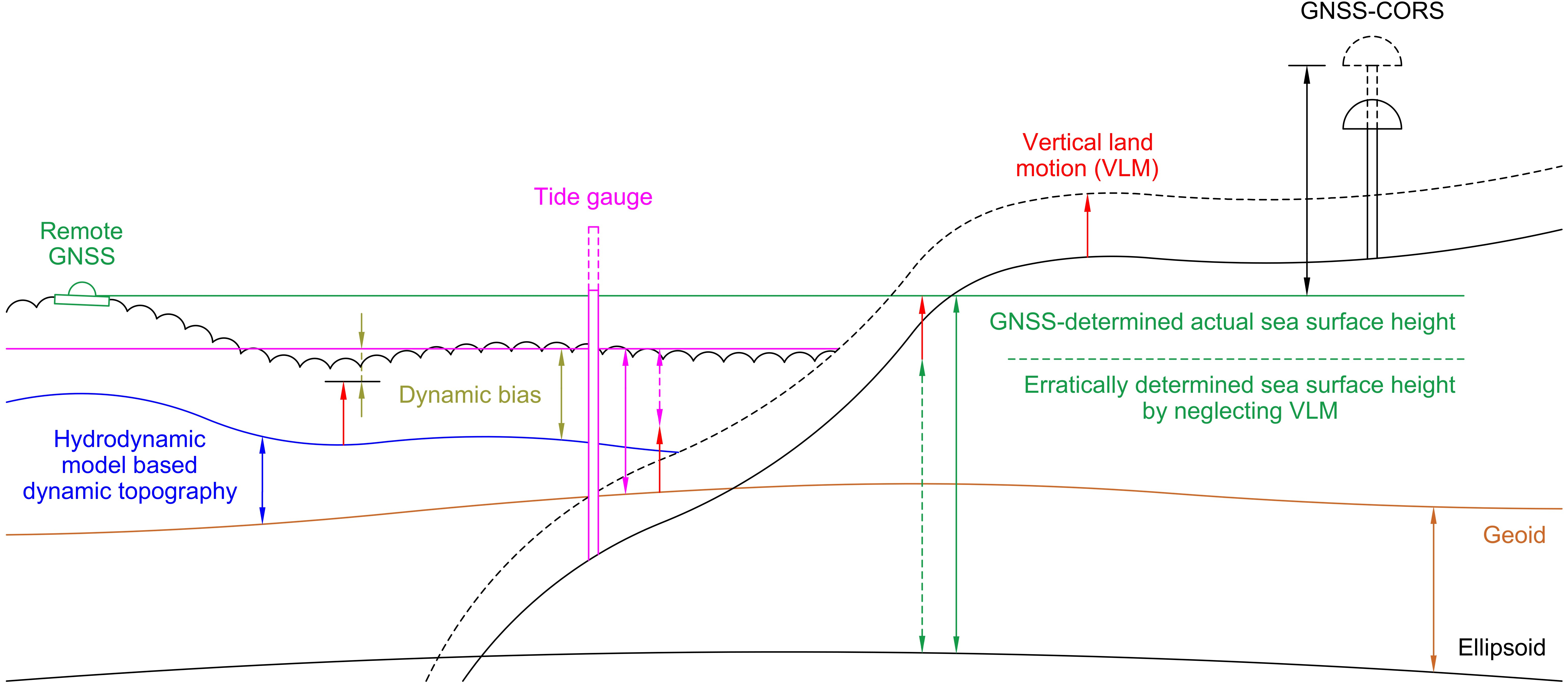
2. Theoretical Principles

With the knowledge of the vertical range ($R$) between a reference point on a vessel (e.g., GNSS antenna’s reference point) and the sea surface (e.g., determined by a total station survey), instantaneous SSH can be calculated relative to a geodetic reference ellipsoid (e.g., GRS80), using GNSS measured ellipsoidal heights $h$:

$$iSSH\left(\phi ,\lambda ,t\right)=h\left(\phi ,\lambda ,t\right)-R,$$

(1)

where $\phi$ and $\lambda$ are the measurement points’ geodetic latitude and longitude at a GNSS observation epoch $t$, respectively. Instantaneous SSH is only an approximation of the actual SSH, as it contains the vessel’s high-frequency attitude changes (e.g., pitch and roll motions) and the impact of sea state (i.e., waves). In addition, vessel sailing-related squat and static draft corrections must be applied, since these cause the vessel to sail with an offset relative to the reference level at which $R$ is usually determined. Accurate derivation of shipborne GNSS-based SSH requires consideration of all these factors.

During GNSS data sampling, an inertial measurement unit can be deployed for specifying the vessel’s attitude [12,32]. However, utilizing an inertial measurement unit may be costly and require dedicated software for data processing. As an alternative, the vessel’s high-frequency attitude changes can be estimated and eliminated from GNSS measurements by using data from at least three GNSS antennas [11,33]. The elimination of the vessel’s high-frequency attitude changes, by computing a joint height solution from multiple antennas to the vessel’s mass center, is further discussed in Section 5.1, with a complementing data example.

Note that such a joint height solution from multiple antennas retains the impact of waves, which manifests itself as heave motion (i.e., vertical movements of the vessel). The required SSH data can be separated from these height estimates by applying a low-pass filter [11,32]. The filtering window (spatial) length can be several kilometers long, depending on the GNSS data sampling rate, implying that the filter may propagate errors to the resulting SSH data; for instance, in steep geoid gradient areas. Therefore, the heights should be reduced to residual values prior to low-pass filtering:

$$r^{UF}\left(\phi ,\lambda ,t\right)=iSSH\left(\phi ,\lambda ,t\right)-\widehat{DT}\left(\phi ,\lambda ,t\right)-N\left(\phi ,\lambda \right),$$

(2)

where $r^{UF}$ denotes unfiltered residual values. The term $\widehat{DT}$ denotes the ever-changing DT during a shipborne GNSS survey and $N$ geoidal heights. The latter can be obtained from a suitable geoid model, whereas DT must be estimated.

As already discussed in the Introduction, the combination of TG and HDM datasets allows DT estimation [15,30]. First, the DB values of an HDM are determined at the locations of TG stations:

$$DB\left({\phi }^{TG},{\lambda }^{TG},t\right)=D{T}_{HDM}\left({\phi }^{TG},{\lambda }^{TG},t\right)-D{T}_{TG}\left({\phi }^{TG},{\lambda }^{TG},t\right),$$

(3)

where $D{T}_{HDM}$ and $D{T}_{TG}$ are HDM- and TG-based DT, respectively (see also Figure 1). With a suitable spatial interpolation method, the DB estimates are then gridded with HDM resolution. These predicted offshore DB ($\widehat{DB}$) provide correction to the initial HDM:

$$\widehat{DT}\left({\phi }^{HDM},{\lambda }^{HDM},t\right)=D{T}_{HDM}\left({\phi }^{HDM},{\lambda }^{HDM},t\right)-\widehat{DB}\left({\phi }^{HDM},{\lambda }^{HDM},t\right),$$

(4)

where $\widehat{DT}$ denotes the corrected HDM-based DT. Dynamic topography at the GNSS measurement locations can finally be estimated via bilinear interpolation. Derivation of offshore DT is further discussed in Section 4, with accompanying data processing examples. Similarly, Section 5.2 further examines the low-pass filtering of the residual values.

The above computations result in filtered residual values $r^F$, which should be corrected for vessel sailing-related effects, such as squat and static draft:

$$r^{F+C}\left(\phi ,\lambda ,t\right)=r^F\left(\phi ,\lambda ,t\right)-C\left(t\right),$$

(5)

where the term $C$ denotes the vessel sailing-related corrections collectively. Section 5.3 presents an example of their empirical derivation. Ideally, the resulting filtered and corrected residuals $r^{F+C}$ should be near-zero, but such results cannot be expected, due to measurement errors and deficiencies in the used models. Thus, the residual values provide means for validation. Assuming that the estimated DT, geoid model, and vessel sailing-related corrections are accurate, the residuals primarily represent errors of the GNSS-determined SSH. Finally, the corrected SSH can be restored from the filtered and corrected residuals:

$$SS{H}^{F+C}\left(\phi ,\lambda ,t\right)=r^{F+C}\left(\phi ,\lambda ,t\right)+\widehat{DT}\left(\phi ,\lambda ,t\right)+N\left(\phi ,\lambda \right),$$

(6)

whereby these results are now suitable for further SSH data applications.

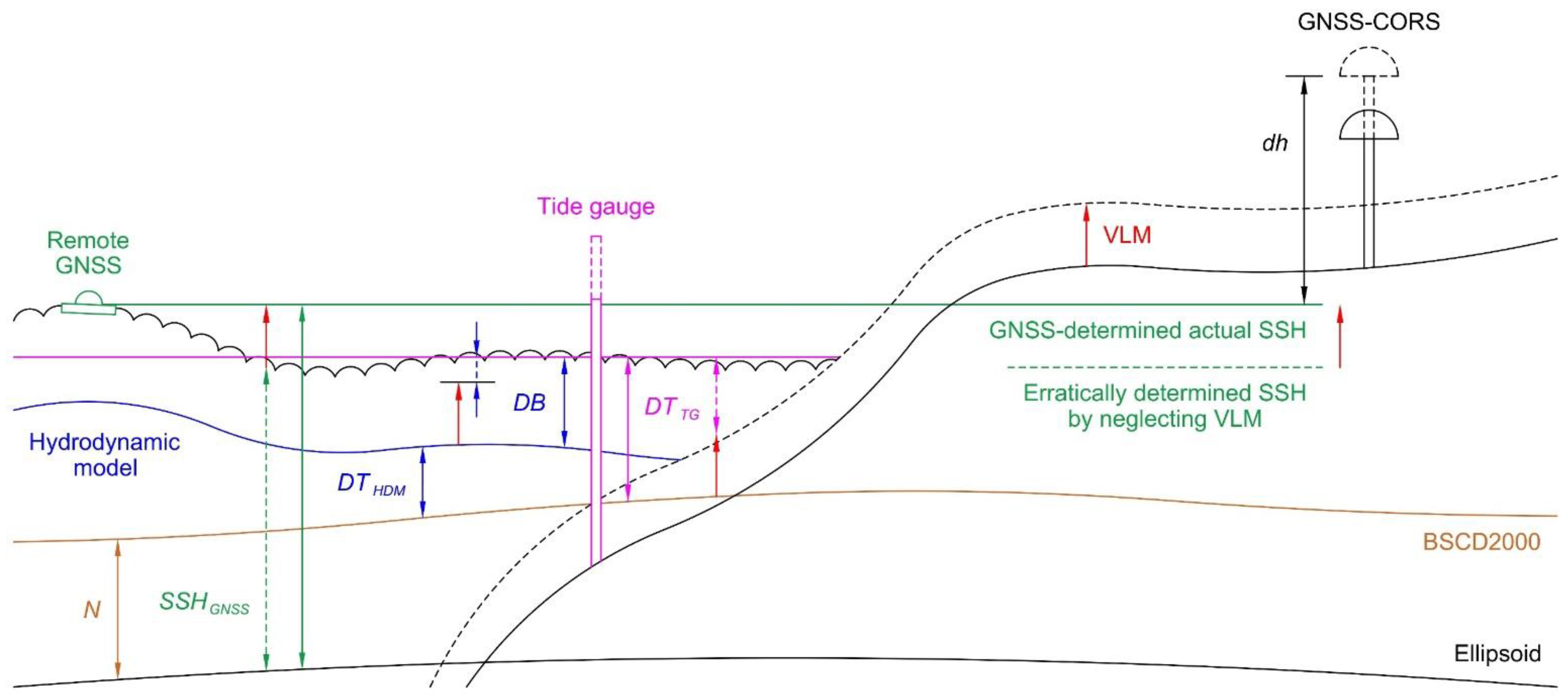
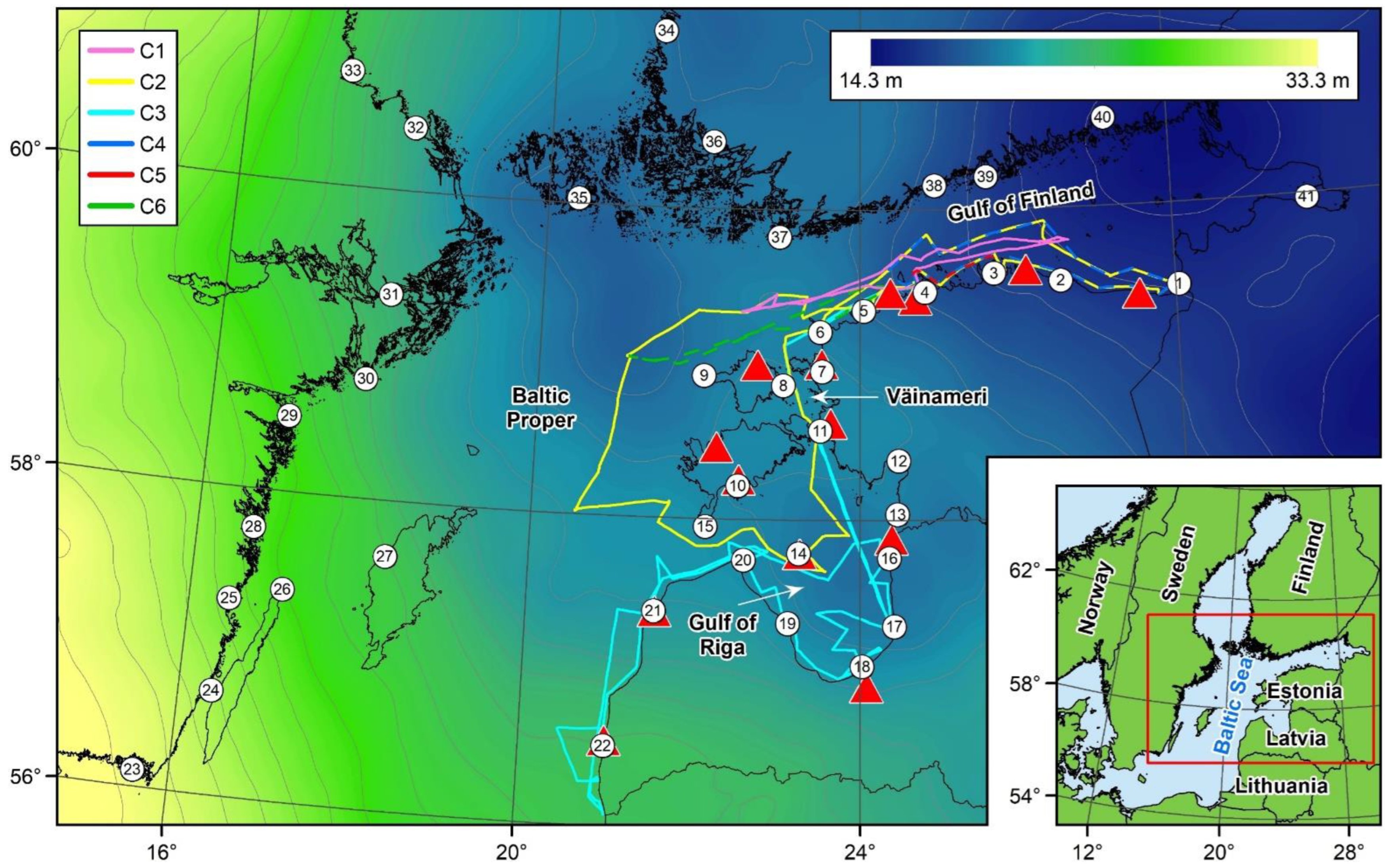
3. Shipborne GNSS Surveys, Data, and Other Used Information

Six marine survey campaigns were conducted in the Eastern Baltic Sea in the spring and summer of 2021 (

Table 1. General information about the conducted marine survey campaigns.

Campaign Identifier	Month (GPS Week)	Duration of a Campaign (h)	Route Length of a Campaign (km)	Number of HDM Grids/DT Computation Duration (h)	Number of Computed SSH Data Points	Temporal Resolution of SSH (s)
C1	April (2152)	52	544	120	11,908	15
C2	July (2168)	106	1439	168	12,253	30
C3	August (2169)	146	1874	192	16,222	30
C4	August (2172)	40	515	96	4390	30
C5	September (2174)	9	98	96	832	30
C6	September (2175)	40	454	120	4449	30

and Figure 2). Each campaign had a primary objective related to different Tallinn University of Technology marine condition monitoring projects. For instance, some tasks involved collecting water samples (e.g., chlorophyll, turbidity, nutrients, phytoplankton), measuring the vertical profiles of water properties (e.g., temperature, salinity, oxygen, light attenuation), or servicing marine monitoring stations. Concurrently, ellipsoidal heights were measured autonomously by four vessel-installed GNSS devices (the used instrumentation is described in [23]). The multi-frequency GNSS receivers were turned on before the vessel left the harbor, and the stored data were downloaded upon returning. During the campaigns, no dedicated GNSS operator was on-board. The GNSS sampling rates were 15 s for the first C1 campaign and 30 s for subsequent campaigns.

The collected shipborne GNSS data were post-processed relative to the Estonian [34] and Latvian [35] national GNSS continuously operating reference stations (CORS) with the commercial Trimble Business Centre software (version 5.52; Trimble Inc., Sunnyvale, CA, USA). Precise GNSS ephemerides (final orbits) from the International GNSS Service were incorporated into post-processing. Since Trimble Business Centre allows only one base station at a time for kinematic data post-processing, the closest GNSS-CORS (cf. Figure 2) was always employed for a GNSS data point computation (similarly to [11,24]). The GNSS-CORS coordinates were fixed to the reference epochs of the national reference frames (i.e., the standard data processing scheme was used). However, the Baltic Sea region’s geodetic networks are deforming, primarily due to glacial isostatic adjustment induced vertical land motion (VLM). The VLM generates discrepancies between the reference and observation epoch positions of a GNSS-CORS, consequently introducing an offset to the marine GNSS measurements (cf. Figure 1), since sea level trends do not follow the VLM directly (but do contain the glacial isostatic adjustment induced geoid change). The neglected VLM correction may, thus, yield lower than actual SSH in the land uplift regions. By employing the principles outlined in [26], the GNSS measurements were corrected retrospectively for VLM occurring at the GNSS-CORS:

$$h\left(\phi ,\lambda ,t,t_0\right)=h_0\left({\phi }^{RS},{\lambda }^{RS},t_0\right)+dh\left(t\right)+\left[VL{M}_{geocentric}\left({\phi }^{RS},{\lambda }^{RS}\right)-GC\left(\phi ,\lambda \right)\right]·\left(t-t_0\right),$$

(7)

where $h_0$ is the ellipsoidal height of a reference station at a reference epoch $t_0$, and $dh$ represents the estimated height difference between a reference station and remote GNSS measurement at an observation epoch $t$. The term $VL{M}_{geocentric}$ denotes the geocentric VLM rate at a GNSS reference station, and $GC$ is the geoid change rate at a GNSS measurement location. The VLM and geoid change rates were obtained from the NKG2016LU VLM model [36].

It became evident during GNSS post-processing that some of the vessel’s routes were too distant from the GNSS-CORS (westernmost routes in the Baltic Proper shown in Figure 2), resulting in reduced post-processed data quality. Previous studies [24,37,38] have shown that the Canadian CSRS-PPP online global precise point positioning service [39] can provide reliable post-processing for remote shipborne GNSS measurements. In particular [37], demonstrated that CSRS-PPP is a viable option for post-processing GNSS data, even in a transoceanic scenario for determining SSH. The results in [23] indicate that CSRS-PPP-based data are consistent, regardless of the distance from the coast and, thus, suitable for complementing poor-performing Trimble Business Centre post-processed route sections. Therefore, the poor-performing sections were replaced by CSRS-PPP solutions.

The results of a total station survey and tape measurements (in the harbor) allowed reducing the post-processed and VLM corrected GNSS ellipsoidal heights to the sea surface. The four GNSS antennas’ reference points and three benchmarks on the vessel’s railing were assigned coordinates in an arbitrary local system, whereby tape measurements (conducted separately for each campaign) determined the vertical distances between benchmarks and the sea surface. The ellipsoidal heights $h$ obtained using Equation (7) were transformed into instantaneous SSH as (Equation (1) modification):

$$iSSH\left(\phi ,\lambda ,t,t_0\right)=h\left(\phi ,\lambda ,t,t_0\right)-H_{TS}^{ARP}+H_{TS}^{BM}-H_{tape}^{BM},$$

(8)

where $H_{TS}^{ARP}$ and $H_{TS}^{BM}$ denote the total station determined heights of an antenna’s reference point and a benchmark on the railing, respectively, and $H_{tape}^{BM}$ is a distance measured by tape. Additional details about the total station survey and instantaneous SSH calculations can be found in [23].

This contribution now aims to further process the instantaneous SSH data, so that these are suitable for subsequent applications (e.g., validation of SA results, marine geoid models, HDMs’ performance). However, Section 4 first examines the derivation of offshore DT, since SSH computations were performed jointly with data validation, which also requires geoidal heights. The latter were obtained from the high-resolution (0.01 × 0.02 arc-deg, i.e., approximately 0.6 nautical miles) NKG2015 quasigeoid (over marine areas, the geoid coincides with the quasigeoid; henceforth, the shorter term will be used) model [40] (cf. Figure 2). Note that NKG2015 represents a geoid model using the zero-tide permanent tide concept, to which a correction from zero-tide to the tide-free concept has been applied (see [41,42] for details about permanent tide concepts). The correction provides consistency with GNSS measurements (using the tide-free concept). In other words, by subtracting NKG2015 heights from the GNSS determined ellipsoidal heights, normal heights using the zero-tide concept are obtained.

Hydrodynamic Model and Tide Gauge Data

Previous works [11,15,30,43] have evaluated the ability of the various HDMs available for the Baltic Sea in deriving sea surface dynamics. Based on these assessments, all the models contain a DB relative to the used height reference (i.e., BSCD2000), whereby the bias varies between models. It also appears that, generally, the most accurate representation of sea surface dynamics in the region can be obtained from the high-resolution (hourly data, with a spatial resolution of approximately 1.0 nautical miles) NEMO-Nordic model [44,45], which was, thus, also chosen for DT determination in this study. If TGs are connected (e.g., by geodetic leveling) to the used height system(s), the DB in the NEMO-Nordic-based DT can be estimated using TG readings. This study employed hourly data from 41 TG stations: 15 Estonian, 7 Latvian [46], 11 Swedish [47], 7 Finnish [48], and one Russian [49] (cf. Figure 2). Note that the NEMO-Nordic model and Russian TG data should be first converted from mean-tide to the zero-tide permanent tide concept for compatibility with the Estonian, Latvian, Swedish, and Finnish TG data [26] (and the normal heights discussed at the end of the previous section). Moreover, the Latvian [50] and Finnish [26,51] TG readings are initially given relative to alternative height reference levels. Hence, before utilization, these data must be converted relative to the used height reference (i.e., national height systems compatible with the BSCD2000).

Even though the Estonian, Latvian, Swedish, and Finnish height systems are all EVRS-based and heights refer to the Normaal Amsterdams Peil (NAP), some minor discrepancies exist (an additional discussion can be found in [26]). Thus, the pan-continental EVRF2019 [52] solution-based height system discrepancies can improve TG data compatibility further. Since GNSS post-processing was conducted relative to the Estonian and Latvian GNSS-CORS, the respective height systems were considered the zero level. The EVRF2019 solution yielded a −1 cm correction to the Swedish and Finnish TG readings. On the other hand, the Russian TG data are given relative to the Baltic Height System of 1977 (BHS77), and a +21 cm offset had to be added.

Similarly to the geodetic networks, the Baltic Sea TG networks are also deforming due to VLM. Even though the zeros of TGs approximately coincide with the reference level at the (common) reference epoch of the national height systems, in the land uplift regions, the zero separates from the reference, yielding lower than actual sea level readings (i.e., DT relative to the nearby solid Earth; cf. Figure 1). The principles outlined in [26] were, hence, employed to obtain absolute DT (i.e., relative to the height reference):

$$D{T}_{TG}\left({\phi }^{TG},{\lambda }^{TG},t^H\right)=D{T}_{RSL}\left({\phi }^{TG},{\lambda }^{TG},t^H,t_0\right)+VL{M}_{leveled}\left({\phi }^{TG},{\lambda }^{TG}\right)·\left(t^H-t_0\right),$$

(9)

where $D{T}_{TG}$ and $D{T}_{RSL}$ are the TG-based absolute and relative DT at an observation epoch $t^H$ (hourly temporal resolution), respectively, and $VL{M}_{leveled}$ denotes leveled VLM rate at a TG station (obtained from the NKG2016LU VLM model). The term $t_0$ denotes the reference epoch of a height system to which the derived $D{T}_{TG}$ refers. These TG data, corrected for datum offsets and VLM, were then used for linking the NEMO-Nordic HDM to the used height references for offshore DT derivation.

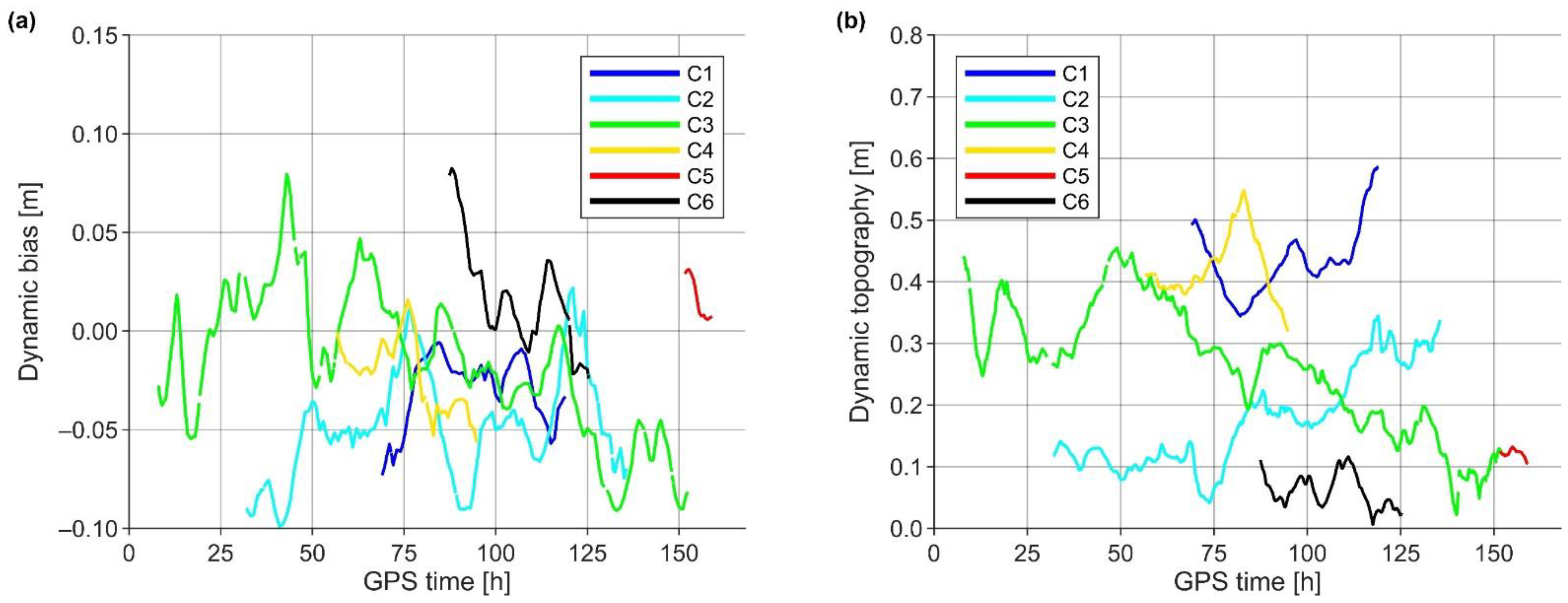
4. Derivation of Offshore Dynamic Topography

Dynamic topography, defined as the SSH and marine geoid separation, represents one of the most valuable parameters, in terms of marine dynamics. Accurate knowledge of DT can guarantee safe navigation at sea, help understand oceanographic processes, and be combined with a suitable geoid model to validate various SSH measurements. With the method developed by [15,30], TG data and an HDM can be combined using Equation (3) to estimate the HDM-contained DB values at the locations of TG stations (at hourly temporal resolution $t^H$). Both studies used exact interpolators for DB gridding, which inherently assumes errorless TG data and TGs connections to the height system(s), as well as that the estimated DB at a TG station is an expected value for all nearby offshore locations; although, neither is necessarily true. Errors may always exist, due to instrument malfunctions, natural disasters, human errors, or poor maintenance and documentation [53,54]. Such errors propagate to the derived offshore DT when the gridded DB is used to correct the initial HDM. Thus, a new approach utilizing DB qualities was developed for constraining TG data errors in offshore DB prediction.

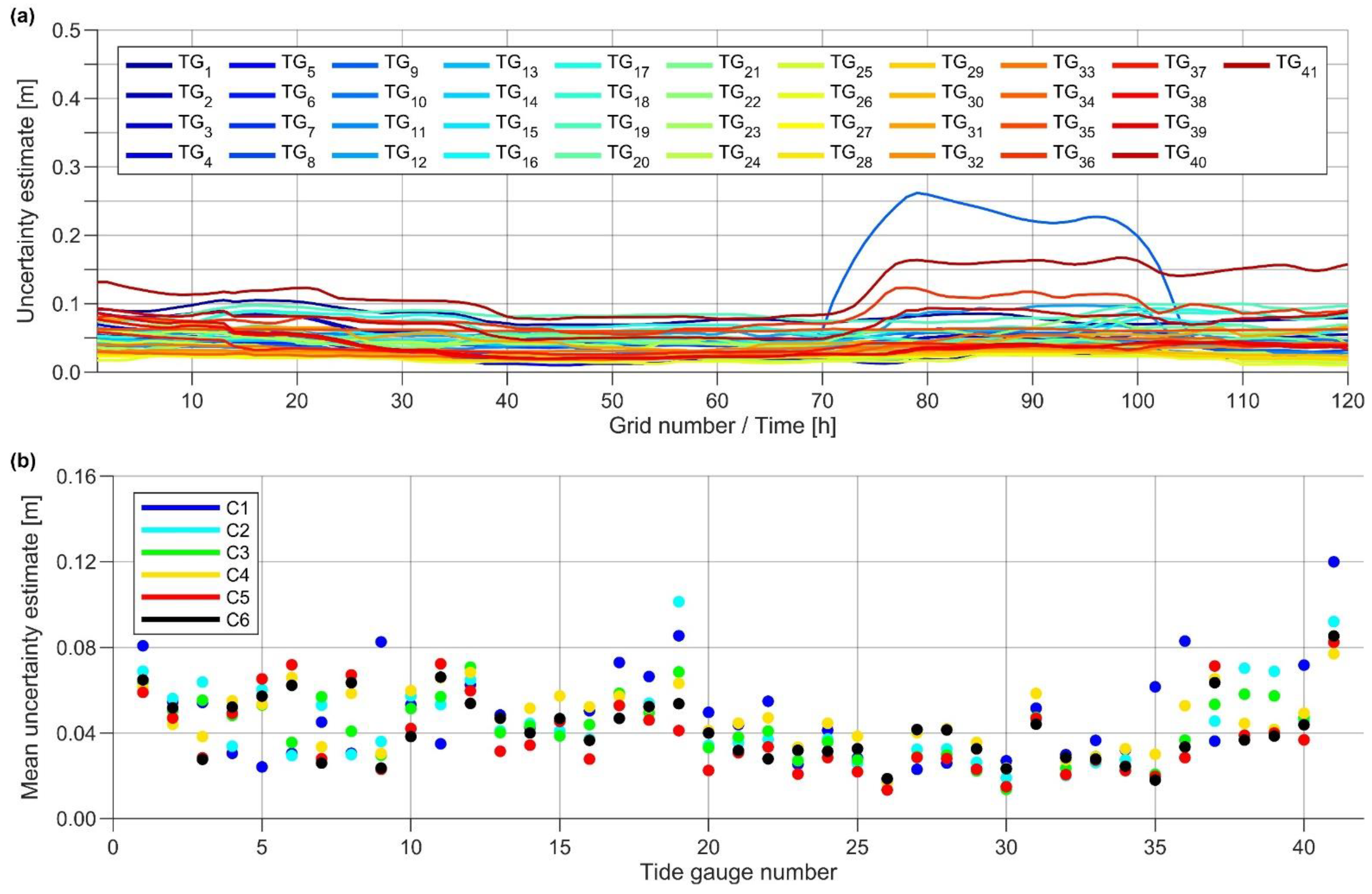
4.1. Estimation of Dynamic Bias Uncertainties at the Tide Gauge Locations

Although DB changes temporally, over short timeframes (e.g., daily), the DB should remain relatively stable, as erratic behavior (such as sudden jumps, both spatially and temporally) would suggest a lack of consistency in the HDM-based DT. However, such a hypothesis first assumes a well-performing HDM (i.e., the HDM phases should match TG data). Figure 3 shows correlation coefficients between the NEMO-Nordic HDM and TG readings at the TG locations. It can be noticed that the (uncorrected) HDM-based DT is well correlated with the TG data, with coefficients being generally above 0.95. The only slight exception is TG₃₁ (refer to Figure 2), with a correlation coefficient of 0.87, likely due to its location in relatively confined waters. The NEMO-Nordic HDM phases, thus, appear to adequately match TG readings (also see [30]).

High DB standard deviation of NEMO-Nordic HDM may, hence, reveal poorly-performing TGs. For instance, notice in Figure 4b the high DB variability at TG₉ and TG₄₁ (yellow dots; also refer to Figure 2) during the C1 campaign, whereas during the C2 (Figure 4d) and C6 (Figure 4f) campaigns, the DB remained relatively stable. Such behavior may be associated with stormy conditions during the second half of the C1 campaign, since the harbor of TG₉ is relatively vulnerable to extreme weather, and TG₄₁ is affected by westerly winds that rapidly accumulate water during storms. Described variations in a confined harbor may not represent the offshore conditions. Therefore, the first uncertainty component (${\sigma }_1$) for DB was estimated as a moving standard deviation (centered at an observation epoch $t^H$) in the DB temporal domain:

$${\sigma }_1\left(t^H\right)=\sqrt{\frac{1}{T-1}{\displaystyle \sum }_{m=t^H-\frac{T-1}{2}}^{t^H+\frac{T-1}{2}}{\left[DB\left({\phi }^{TG},{\lambda }^{TG},m\right)-\frac{1}{T}{\displaystyle \sum }_{m=t^H-\frac{T-1}{2}}^{t^H+\frac{T-1}{2}}DB\left({\phi }^{TG},{\lambda }^{TG},m\right)\right]}^2},$$

(10)

where $T$ denotes the time extent considered at a certain time. A 25-h period was determined suitable, whereby a minimum of 12 h of data was included in all DB (and DT) computations, before and after the campaigns. This was done to avoid shorter than 25 h window sizes during the campaigns, which would have introduced inconsistency to the temporal domain uncertainty estimation.

Since DB has a long-wavelength nature, the mean DB estimates at neighboring TG stations should ideally be similar in value. Therefore, discrepancies between mean DB estimates may reveal, for example, errors in TGs connections to height system(s) or near-shore processes. In the Gulf of Riga (cf. Figure 2), the mean DB estimates differ over relatively short spatial scales (Figure 4a,c,e); whereby, the discrepancies appear similar during all the campaigns. For instance, the mean DB at TG₁₇ always appears higher than at TG₁₆ and TG₁₈ (refer to Figure 2). A higher mean DB estimate can similarly be observed at TG₄₀. Such reoccurring discrepancies could indicate errors in the levelings that connect TGs to height system(s).

Alternatively, the mean DB at TG₁₄ (refer to Figure 2) was significantly higher (more than usual) than at the neighboring TG stations during the C2 campaign (Figure 4c). According to the nearby weather station, during the second half of the C2 campaign, relatively strong winds (occasionally over 10 m/s) blew in the general direction of the exit of the harbor in which TG₁₄ resides. The receding water level in the harbor may, thus, have been a cause for a high mean DB estimate. Such behavior, however, does not represent offshore marine processes. Additionally [23], compared TG₄ readings to DT determined at the vessel’s harbor, roughly 5 km away. It was demonstrated that the DT could differ by up to 8–9 cm between two nearby sheltered locations. According to the [15] and [30] approach, TG₄ data would represent the DT at the harbor.

In predicting offshore DB, the described potential offsets should be considered. Hence, the second uncertainty component (${\sigma }_2$) was estimated by first comparing mean DB values at neighboring TG stations. These comparisons yielded $N$ discrepancy estimates $\overline{dDB}$ for each mean DB value (i.e., mean discrepancies). The second uncertainty component was then estimated in the DB spatial domain as:

$${\sigma }_2=\sqrt{\frac{1}{N-1}{\displaystyle \sum }_{m=1}^N{\left[{\overline{dDB}}_m\left({\phi }^{TG},{\lambda }^{TG}\right)-\frac{1}{N}{\displaystyle \sum }_{m=1}^N{\overline{dDB}}_m\left({\phi }^{TG},{\lambda }^{TG}\right)\right]}^2},$$

(11)

It was determined that comparisons with mean DB estimates at the nearest three TG stations (by also considering the distribution of TG stations) provided satisfactory results (i.e., $N=3$). Note that the second uncertainty component was calculated separately for each campaign (e.g., for campaign C1, precisely the values shown in Figure 4a were used), whereby the mean DB values were estimated over an extended period. For example, the 9-h length of campaign C5 may not have been sufficient for calculations, which were therefore performed over a 96-h period instead (cf. Table 1). In studies investigating extensive periods, the second uncertainty component should also be estimated as a moving window (as is done for the first component), because offsets caused by marine processes are not likely to reoccur often (for instance, the TG₁₄ example). Here, this is emulated by a separate estimation for each campaign.

It is assumed that the first (temporal domain) and second (spatial domain) uncertainty components are (generally) independent variables. The final uncertainty estimates for DB were, thus, calculated as:

$${\sigma }_{DB}\left(t^H\right)=\sqrt{{\left[{\sigma }_1\left(t^H\right)\right]}^2+{\left[{\sigma }_2\right]}^2},$$

(12)

where $t^H$ denotes hourly temporal resolution. The resulting DB uncertainties for campaign C1 are shown in Figure 5a. Notice how the estimates at TG₉ increase significantly during the second half of the campaign, which coincides with the period of strongest storm winds (as discussed earlier). The uncertainty estimates are summarized for all campaigns in Figure 5b by averaging. These (hourly resolution) results were next employed in predicting offshore DB.

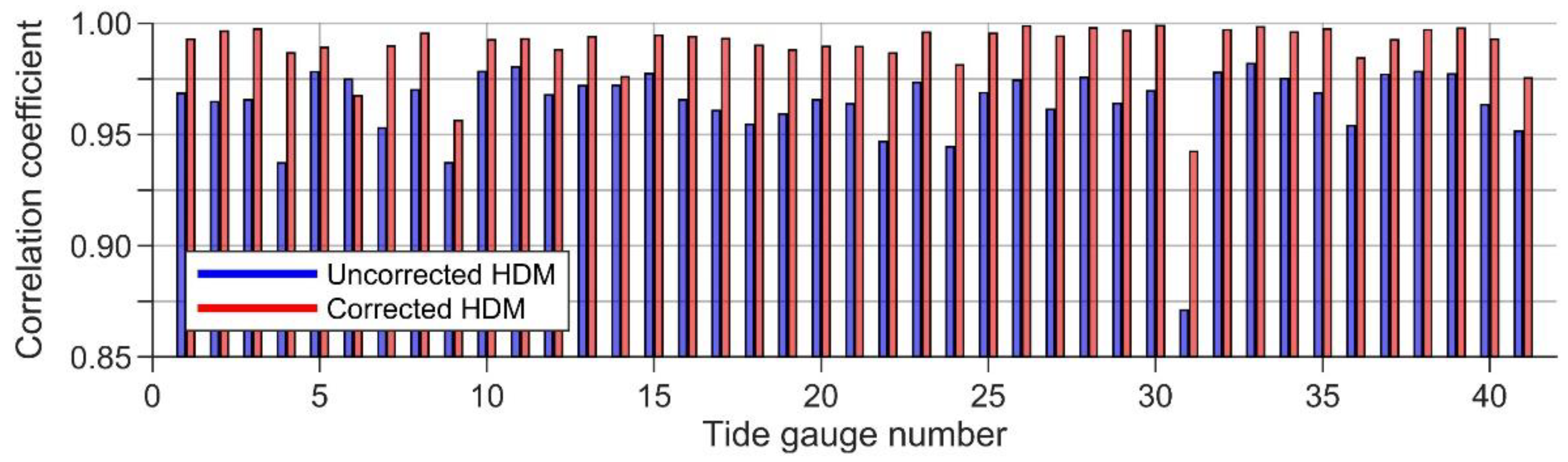
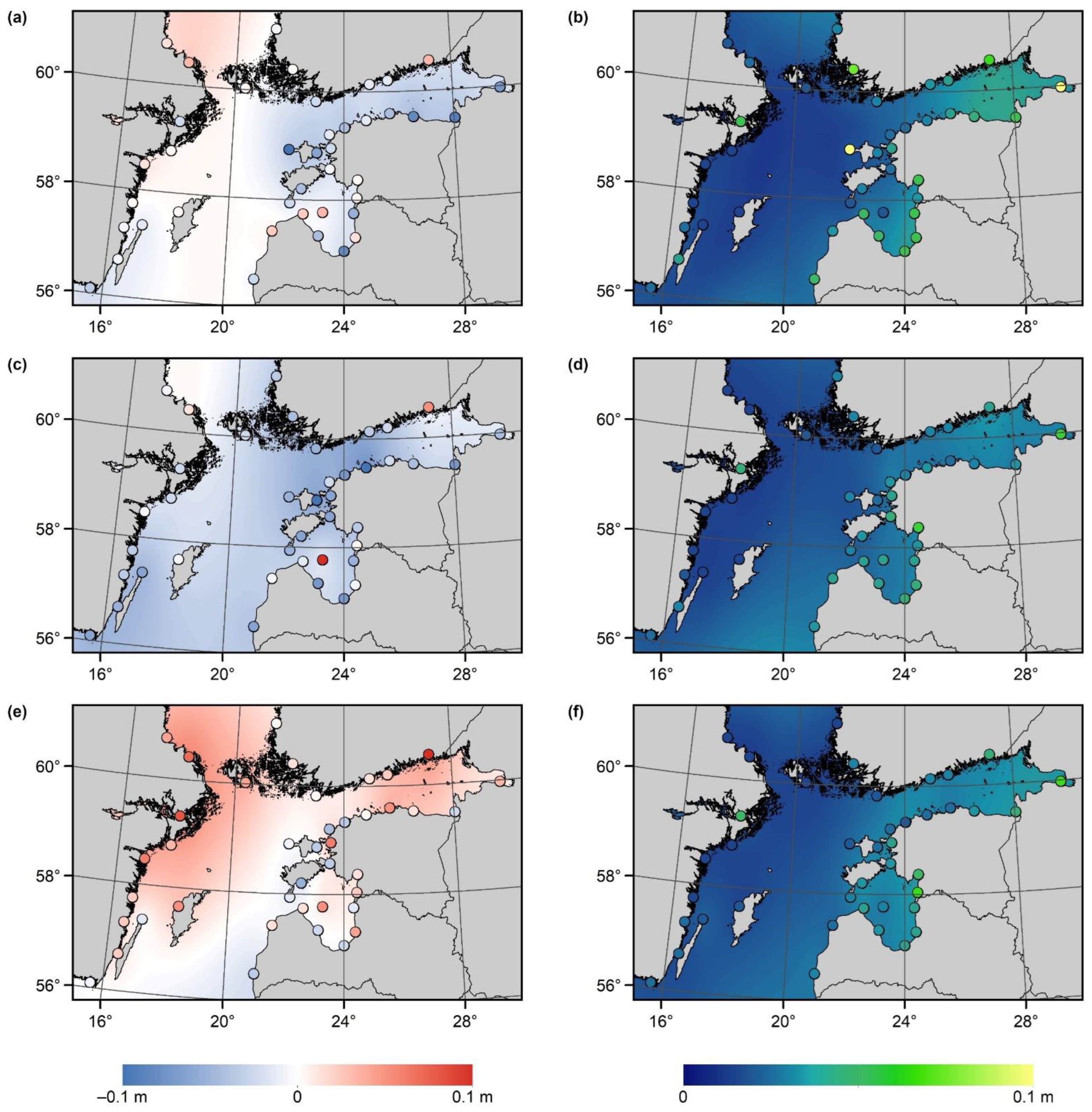
4.2. Correction of Hydrodynamic Model Based Dynamic Topography

With the inclusion of determined uncertainties, the DB estimates were predicted offshore (with the NEMO-Nordic spatial resolution) by employing least-squares collocation [55] with the second-order Markov model covariance function [56]. In Figure 4, the mean predicted DB and standard deviation estimates of predicted DB for campaigns C1, C2, and C6 are presented. The estimated surfaces smoothly follow the long-wavelength DB trends determined at TG locations, but do not include the erratic behavior and offsets described in Section 4.1. It appears that the primary variations of DB occur in the Gulf of Finland and Gulf of Riga, while DB is more stable in the Baltic Proper (Figure 4b,d,f; refer to Figure 2 for basin locations). Additionally, notice how the mean DB surfaces differ for campaigns C1, C2, and C6 (Figure 4a,c,e). These results demonstrate the spatiotemporal changes of the NEMO-Nordic contained DB well.

The predicted offshore DB was used to correct the initial HDM (at hourly temporal resolution $t^H$) by employing Equation (4). Notice that the comparisons between the corrected NEMO-Nordic HDM and TG readings now yield improved correlation coefficients, except for TG₆, which shows a slightly reduced correlation (Figure 3). Since this study aimed to derive and validate shipborne GNSS-based SSH, the DT estimates were finally determined at the GNSS measurement locations via bilinear interpolation at observation epochs $t$ (interpolated linearly from the hourly resolution data). These values are shown in Figure 6b and denoted as $\widehat{DT}\left(\phi ,\lambda ,t\right)$. See also the predicted DB during marine survey campaigns in Figure 6a.

5. Derivation and Validation of Shipborne GNSS-Based Sea Surface Heights

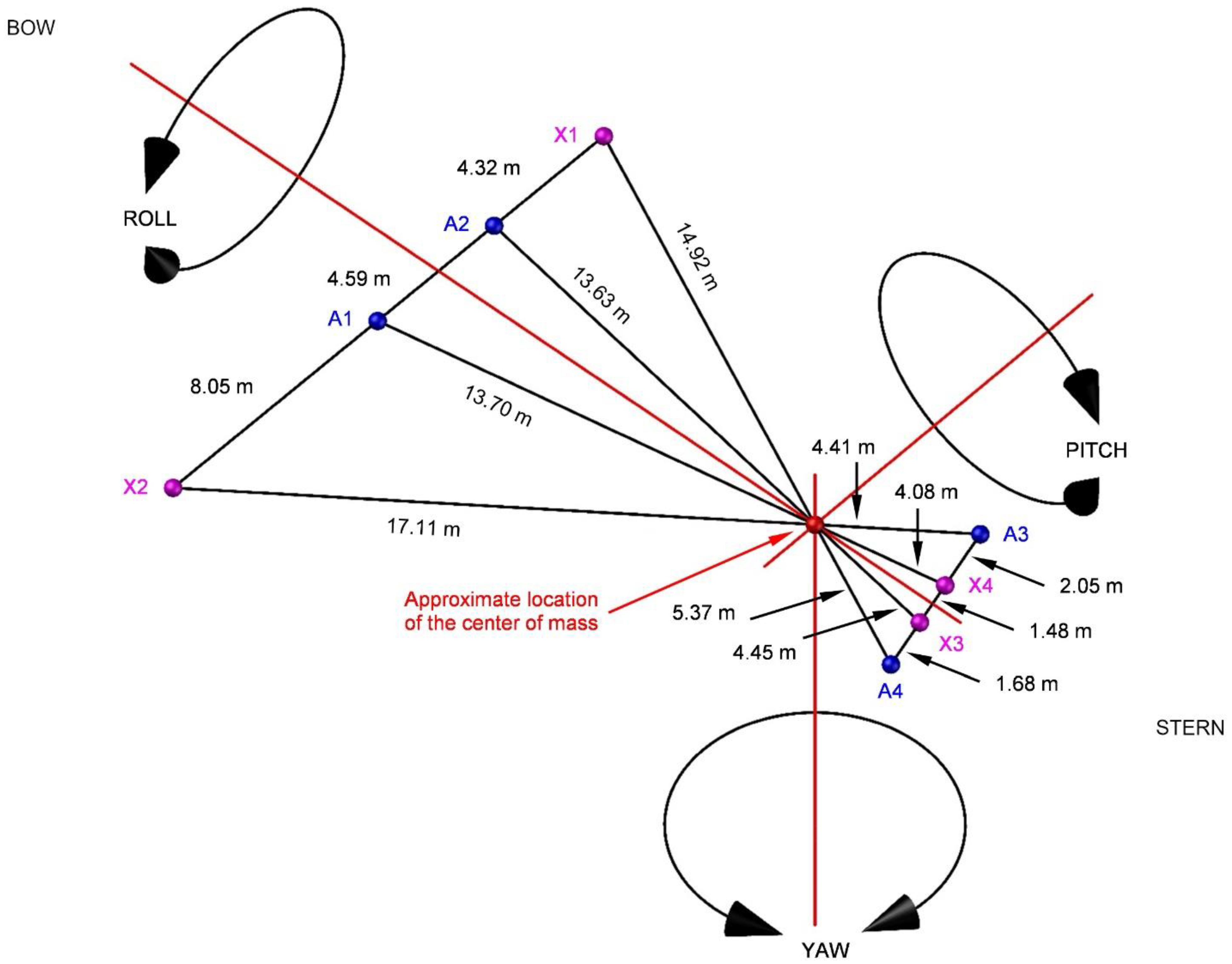
5.1. Reducing the Effects of Vessel’s High-Frequency Attitude Changes

Determination of accurate SSH requires considering the vessel’s pitch and roll motions (Figure 7), where the yaw motion can be neglected, as the focus is on heights. In this study, the approach developed by [11] was improved using an additional GNSS antenna. By computing instantaneous SSH from multiple antennas jointly to the vessel’s stable mass center, the method eliminates (or, at the very least, significantly reduces) the vessel’s high-frequency attitude changes from the joint SSH solution. The distances between GNSS antennas relative to the vessel’s mass center (Figure 7) were derived from total station measurements (see also [23]).

The GNSS determined instantaneous SSH (cf. Equation (8)) from three antennas were first interpolated linearly to the location of the vessel’s center of mass in two steps:

$$iSS{H}_{X\alpha }\left(\phi ,\lambda ,t,t_0\right)=iSS{H}_{A\gamma }\left(\phi ,\lambda ,t,t_0\right)+c_1\left[iSS{H}_{A\left(\gamma +1\right)}\left(\phi ,\lambda ,t,t_0\right)-iSS{H}_{A\gamma }\left(\phi ,\lambda ,t,t_0\right)\right]$$

(13)

$$iSS{H}_{CoM}^{\xi }\left(\phi ,\lambda ,t,t_0\right)=iSS{H}_{X\alpha }\left(\phi ,\lambda ,t,t_0\right)+c_2\left[iSS{H}_{A\left(\left\{1,2,3,4\right\}-\left\{\gamma ,\gamma +1,\xi \right\}\right)}\left(\phi ,\lambda ,t,t_0\right)-iSS{H}_{X\alpha }\left(\phi ,\lambda ,t,t_0\right)\right],$$

(14)

where the index $\alpha$ denotes the number of an imaginary intersection point, the index $\gamma$ number of an antenna and $\xi$ solution numbered according to an excluded fourth antenna (also refer to Figure 7 and

Table 2. The solutions’ ($\xi$ ) associated indexes ($\alpha$, $\beta$, and $\gamma$ ) and coefficient values ($c_1$, $c_2$, $c_3$, and $c_4$; also see Figure 7).

Index/Coefficient	Solution $\mathit{\xi }=1$	Solution $\mathit{\xi }=2$	Solution $\mathit{\xi }=3$	Solution $\mathit{\xi }=4$
$\alpha$	3	4	1	2
$\beta$	4	3	2	1
$\gamma$	3	3	1	1
$c_1$	$\frac{2.05 + 1.48}{2.05 + 1.48 + 1.68}$	$\frac{2.05}{2.05 + 1.48 + 1.68}$	$\frac{4.59 + 4.32}{4.59}$	$\frac{8.05}{-4.59}$
$c_2$	$\frac{4.45}{4.45 + 13.63}$	$\frac{4.08}{4.08 + 13.70}$	$\frac{14.92}{14.92 + 5.37}$	$\frac{17.11}{17.11 + 4.41}$
$c_3$	$\frac{2.05}{2.05 + 1.48 + 1.68}$	$\frac{2.05 + 1.48}{2.05 + 1.48 + 1.68}$	$\frac{8.05}{-4.59}$	$\frac{4.59 + 4.32}{4.59}$
$c_4$	$\frac{4.08 + 13.70}{4.08}$	$\frac{4.45 + 13.63}{4.45}$	$\frac{17.11 + 4.41}{17.11}$	$\frac{14.92 + 5.37}{14.92}$

). Coefficients $c_1$ and $c_2$ are determined from total station measurement derived distances. The geodetic coordinates ($\phi$, $\lambda$) represent the general location of the vessel (e.g., chosen according to the best performing antenna; in this study, coordinates of the antenna A4 were consistently used), and $t$ is an observation epoch of a GNSS measurement. These calculations resulted in four $iSS{H}_{CoM}^{\xi }$ solutions (i.e., instantaneous SSH at the vessel’s mass center). Unfortunately, such calculations were not possible for the C4 campaign, due to the malfunctioning of two instruments [23]. For the C4 campaign, the instantaneous SSH of antennas A1 and A2 were averaged at observation epochs $t$.

Since the four antennas form a rigid system, the instantaneous SSH at the vessel’s mass center can be further used for validation purposes. Hence, the instantaneous SSH estimates at the previously excluded fourth antenna location were interpolated similarly:

$$iSS{H}_{X\beta }\left(\phi ,\lambda ,t,t_0\right)=iSS{H}_{A\gamma }\left(\phi ,\lambda ,t,t_0\right)+c_3\left[iSS{H}_{A\left(\gamma +1\right)}\left(\phi ,\lambda ,t,t_0\right)-iSS{H}_{A\gamma }\left(\phi ,\lambda ,t,t_0\right)\right]$$

(15)

$$i{\widehat{SSH}}_{A\xi }\left(\phi ,\lambda ,t,t_0\right)=iSS{H}_{X\beta }\left(\phi ,\lambda ,t,t_0\right)+c_4\left[iSS{H}_{CoM}^{\xi }\left(\phi ,\lambda ,t,t_0\right)-iSS{H}_{X\beta }\left(\phi ,\lambda ,t,t_0\right)\right],$$

(16)

where the index $\beta$ denotes the number of an imaginary intersection point, and coefficients $c_3$ and $c_4$ are determined from total station measurement derived distances (Figure 7 and Table 2). The conducted calculations were validated by comparing the estimated ($i{\widehat{SSH}}_{A\xi }$) and measured ($iSS{H}_{A\xi }$) heights:

$$d_{A\xi }\left(\phi ,\lambda ,t\right)=i{\widehat{SSH}}_{A\xi }\left(\phi ,\lambda ,t,t_0\right)-iSS{H}_{A\xi }\left(\phi ,\lambda ,t,t_0\right),$$

(17)

where $d_{A\xi }$ denotes discrepancies at the location of the initially excluded fourth antenna. Statistics of discrepancies are summarized in Figure 8, indicating the expected GNSS height determination accuracy. It can be noticed that, generally, the discrepancy mean values are sub-centimeter, suggesting the successful reduction of ellipsoidal heights to the sea surface using Equation (8) (i.e., all four antennas are approximately on the same plane). Note that the weighted mean (according to campaign distances presented in Table 1) standard deviation estimate (by averaging the values shown in Figure 8) of 4.1 cm showed a good performance for height determination.

Ideally, all four $iSS{H}_{CoM}^{\xi }$ solutions should be free of vessel high-frequency attitude changes and have matching results considering the successful reduction of ellipsoidal heights. The performance of $iSS{H}_{CoM}^{\xi }$ was evaluated as:

$${\overline{\sigma }}_{CoM}=\frac{1}{I}{\displaystyle \sum }_{i=1}^I\left\{\sqrt{\frac{1}{3}{\displaystyle \sum }_{\xi =1}^4{\left[iSS{H}_{CoM}^{\xi }\left(\phi ,\lambda ,i,t_0\right)-\frac{1}{4}{\displaystyle \sum }_{\xi =1}^{4}iSS{H}_{CoM}^{\xi }\left(\phi ,\lambda ,i,t_0\right)\right]}^2}\right\},$$

(18)

where $i=1, 2, \dots , I$ is the number of a GNSS observation. These evaluation results vary between 0.4 cm (C5 campaign) and 1.1 cm (C1 campaign), indicating excellent agreement between the four solutions for all campaigns. Even though the C2 campaign validation suggests more significant (than usual) discrepancies at the antenna locations (Figure 8), the solutions agree well at the vessel’s mass center (${\overline{\sigma }}_{CoM}$ is 0.8 cm). In practical applications use of three GNSS antennas, thus, appears sufficient, and any of the four $iSS{H}_{CoM}^{\xi }$ solutions would be equally suitable for further use. Due to data availability, the final instantaneous SSH solution was calculated as:

$$iSS{H}_{CoM}^{Final}\left(\phi ,\lambda ,t,t_0\right)=\frac{1}{4}{\displaystyle \sum }_{\xi =1}^{4}iSS{H}_{CoM}^{\xi }\left(\phi ,\lambda ,t,t_0\right)$$

(19)

and used in subsequent data filtering. The temporal resolutions of $iSS{H}_{CoM}^{Final}$ were 15 s for the first C1 campaign and 30 s for subsequent campaigns. Recall that the $iSS{H}_{CoM}^{Final}$ of campaign C4 is a simple average of the A1 and A2 antenna heights.

5.2. Reducing the Effects of Sea State Conditions

The computed instantaneous SSH, now with a substantially reduced impact from the vessel’s high-frequency attitude changes (i.e., pitch and roll motions), still contains some influence from sea state conditions (i.e., waves), which primarily manifest as the vessel’s up–down direction heave motion. As a result, instantaneous SSH contains high-frequency variations that should be eliminated from the expected SSH; for instance, by applying a low-pass filter. This study used the approach developed by [24] and successfully employed by [11]:

$$OUT\left(i\right)=\frac{1}{F}{\displaystyle \sum }_{m_2=m_1-\frac{F-1}{2}}^{m_1+\frac{F-1}{2}}Media{n}_{m_2}\left\{I{N}_{m_1}\left(i\right)|i-\frac{F-1}{2}\le m_1\le i+\frac{F-1}{2}\right\},$$

(20)

where $IN$ and $OUT$ denote input and output data, respectively, and $F$ is the filtering window size (i.e., a certain number of measurements). As in Equation (18), $i$ represents a GNSS observation number.

Refs. [11,24] used the low-pass filter directly on SSH data. Recall the temporal data resolution of 15 or 30 s, which at a vessel velocity of around 9 knots results in a filtering window (spatial) length of several kilometers. With such lengthy window sizes, low-pass filtering may contaminate results, due to the gradients of DT and geoid. Thus, (unfiltered) residual estimates were first calculated from $iSS{H}_{CoM}^{Final}$ using Equation (2) (note that the residuals are not dependent on the reference epoch $t_0$, since this dependency disappears using a compatible geoid model NKG2015). A sum of absolute differences (between unfiltered and filtered signals) function was then compiled for each marine survey campaign, by applying the Equation (20) low-pass filter on unfiltered residuals. Only odd filtering window sizes were considered, and the optimal windows were estimated as sizes where the functions became roughly linear. The results are summarized in Figure 9. For comparability, the functions are normalized according to the maximum values.

Notice that the functions are similar in shape, except for the C5 campaign, which is much shorter than the others (i.e., containing fewer measurements; cf. Table 1). However, the optimal filtering window sizes vary, likely due to approximations assumed during the size determination. For consistency, the final filtering window size (used for all data filtering) was estimated as a weighted mean (according to the campaign distances presented in Table 1) of an individual campaigns’ optimal window sizes. The resulting 53 measurements are almost the same as the window size (51 measurements, at which the filtered data had a similar signal frequency to the geoid) suggested by [11].

Notably, such a filtering approach is independent of temporal data resolution (unless the GNSS sampling rate is very high, i.e., sub-second), since sea state conditions cause random data noise; hence, allowing investigation of the filtering window (spatial) length dependency on the GNSS sampling rate and vessel velocity (Figure 10). Ideally, the filtering window length should approximately match the spatial resolution of the employed model datasets (i.e., geoid model and HDM), to decrease error propagation. At a vessel velocity of 9 knots, this implies a GNSS sampling rate of around 5 s. In this study, the sampling rates were 15 or 30 s, and the filtering window lengths were, correspondingly, roughly 4 and 8 km. Future studies and marine survey campaigns should consider the results in Figure 10.

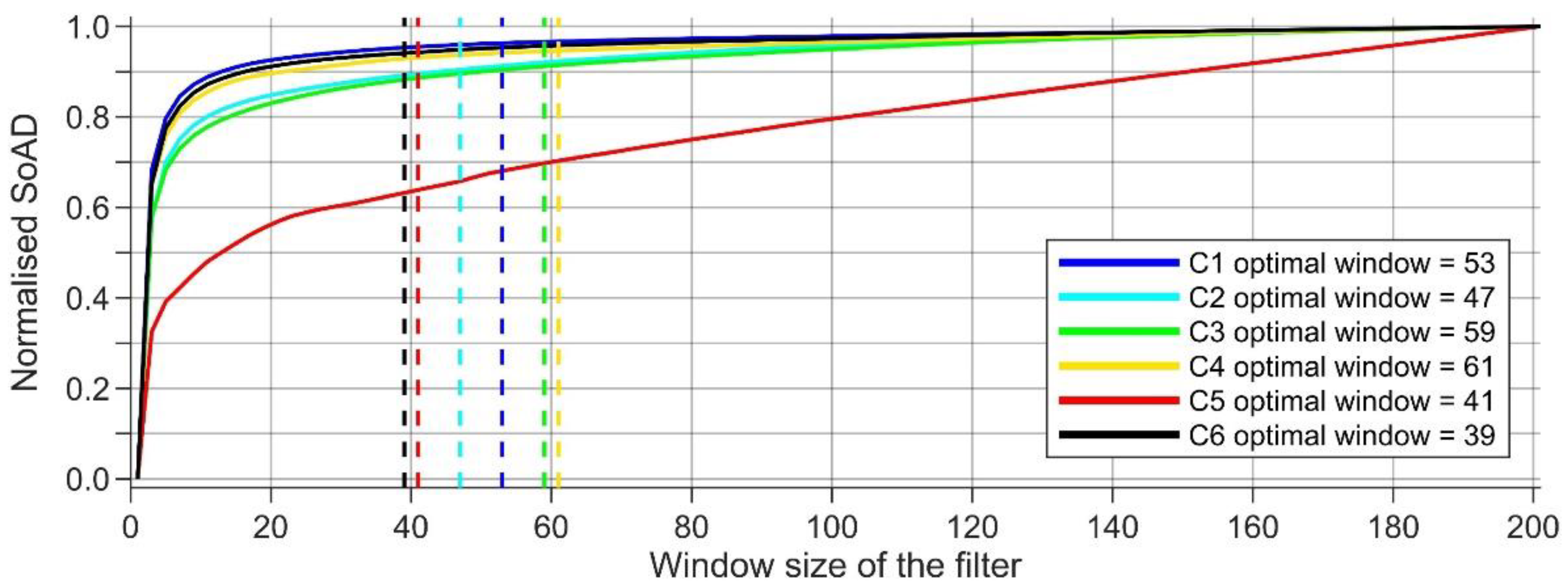
Low-Pass Filtering Results

The Equation (20) low-pass filter, with the filtering window size of 53 measurements, was applied on the unfiltered residuals, resulting in the filtered residuals denoted as $r_{CoM}^F\left(\phi ,\lambda ,t\right)$ in the following. For comparison, the low-pass filter was also used on residuals (also estimated using Equation (2)) determined directly from the instantaneous SSH of individual antennas (i.e., instantaneous SSH from Equation (8)). The results of the C2 campaign before and after data filtering are shown in Figure 11. Notice how the unfiltered residuals of antennas A1 and A2 (at the vessel’s bow) are more scattered than antennas A3 and A4 (and the joint solution), suggesting a dominating pitch motion at the vessel’s bow and that the vessel is more stable near its mass center (cf. Figure 7). Such a revelation implies inferior results for the C4 campaign (recall that the center of mass solution could not be computed).

After filtering, significant discrepancies could be detected between the center of mass and individual antenna solutions (Figure 11b). Residuals of the port side antennas generally appeared lower than starboard antennas’ (a similar pattern can be observed for all other campaigns). The likely cause is the change in the vessel’s general attitude. During total station and tape measurements in the harbor, the vessel was always tilted slightly to the right [23]. The vessel may correct its general attitude while in motion; thus, resulting in lower and higher than actual heights for port and starboard side antennas, respectively. Since the vessel rotates approximately around its mass center, the joint solution $iSS{H}_{CoM}^{Final}$ should consider such a motion.

To further analyze the performance of conducted computations, the unfiltered and filtered residuals were compared (i.e., filtered results were subtracted from unfiltered). The statistics of their differences are summarized in Figure 12. The most significant differences were consistently detected for antennas A1 and A2, again suggesting dominating pitch motion at the vessel’s bow. A reduced standard deviation was always (except for the C4 campaign, which showed no improvement) produced for the mass center solution. In contrast, the low-pass filter eliminated more noise from individual antenna solutions (i.e., resulting in greater differences between unfiltered and filtered residuals). It, hence, appears that the vessel’s high-frequency attitude changes were indeed eliminated (or at the very least significantly reduced) in the $iSS{H}_{CoM}^{Final}$ (cf. Section 5.1).

The described outcomes demonstrate the importance of proper planning for such marine GNSS surveys; the location of the antenna has a significant influence on data accuracy. Before validating this study’s results, vessel sailing-related corrections must be estimated and removed from the filtered residuals. The following section describes their empirical derivation.

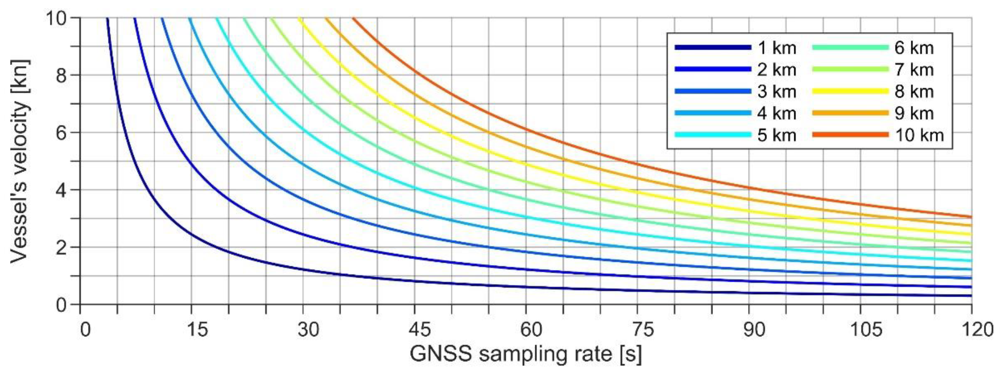
5.3. Vessel Sailing-Related Corrections

In Figure 11b, abnormal peaks can be detected in the C2 campaign mass center solution. These coincide with the occasions of the vessel’s stopping; for example, to collect water samples. This phenomenon occurs due to the disappearance of the squat effect that causes a vessel to sail deeper than its nominal draft. The squat is a function of a vessel’s velocity and dimensions, but is also influenced by depth in shallower, more confined waters [57]. Since the surveys were generally conducted in relatively deep and open marine areas, it is assumed that depth has a negligible influence on the squat. The only slight exception could be campaign C3, which also surveyed shallower regions of the Baltic Sea (notice the near-shore routes in Figure 2).

Due to occasional stops, the velocity could be related to height changes between a moving and static vessel, by utilizing filtered residuals over distances up to 3 km. These estimates that represent squat values at various velocities are presented in Figure 13a as black dots. Since the vessel’s dimensions are constant, the squat is approximately a quadratic velocity function [37,57]. It was, thus, estimated as a least-squares fit of a quadratic function to the empirical data. A linear squat approximation, also shown in Figure 13a, is further discussed in Section 6.4.

The second vessel sailing-related correction that must be considered is the static draft. Due to fuel consumption, the vessel floats gradually higher. The lowest/highest estimates of the static draft are, correspondingly, at the time of harbor departure/return. Thus, the static draft was approximated from differences in tape measurements conducted before and after marine survey campaigns. Since tape measurements may contain errors in the range of static draft itself (e.g., notice the difference between the campaign C4 estimates in Figure 13b), the empirical data were considered altogether, whereas all negative values were excluded. The static draft was then estimated as a distance-related least-squares fit of a linear trend (Figure 13b).

The empirically derived vessel sailing-related squat (a function of the vessel’s velocity $v$) and static draft (a function of the total traveled distance $s$) corrections were subsequently applied to the filtered residuals (Equation (5) modification; also notice the functions presented in Figure 13):

$$\begin{array}{l}{r}_{CoM}^{F+C}\left(\phi ,\lambda ,t\right)=r_{CoM}^F\left(\phi ,\lambda ,t\right)-\left\{squat\left(v\right)\right\}-\left\{static draft\left(s\right)\right\}\\ \hspace{1em}\hspace{1em}\hspace{1em}\hspace{1em}\hspace{1em}\hspace{1em}\hspace{1em} =r_{CoM}^F\left(\phi ,\lambda ,t\right)-\left\{\left(-0.0012\right)·{\left[v\left(t\right)\right]}^2\right\}-\left\{5.95·{10}^{-5}·s\left(t\right)\right\},\end{array}$$

(21)

where the first set of curly braces denotes squat correction, and the second set, static draft correction. The values of $v$ and $s$ are given at a GNSS observation epoch $t$. Note that the vessel’s velocity is considered in knots, and the total traveled distance is in kilometers from the beginning (i.e., home harbor) of the campaign. The term $r_{CoM}^{F+C}$ denotes filtered and corrected residuals, which were validated as described in the following section.

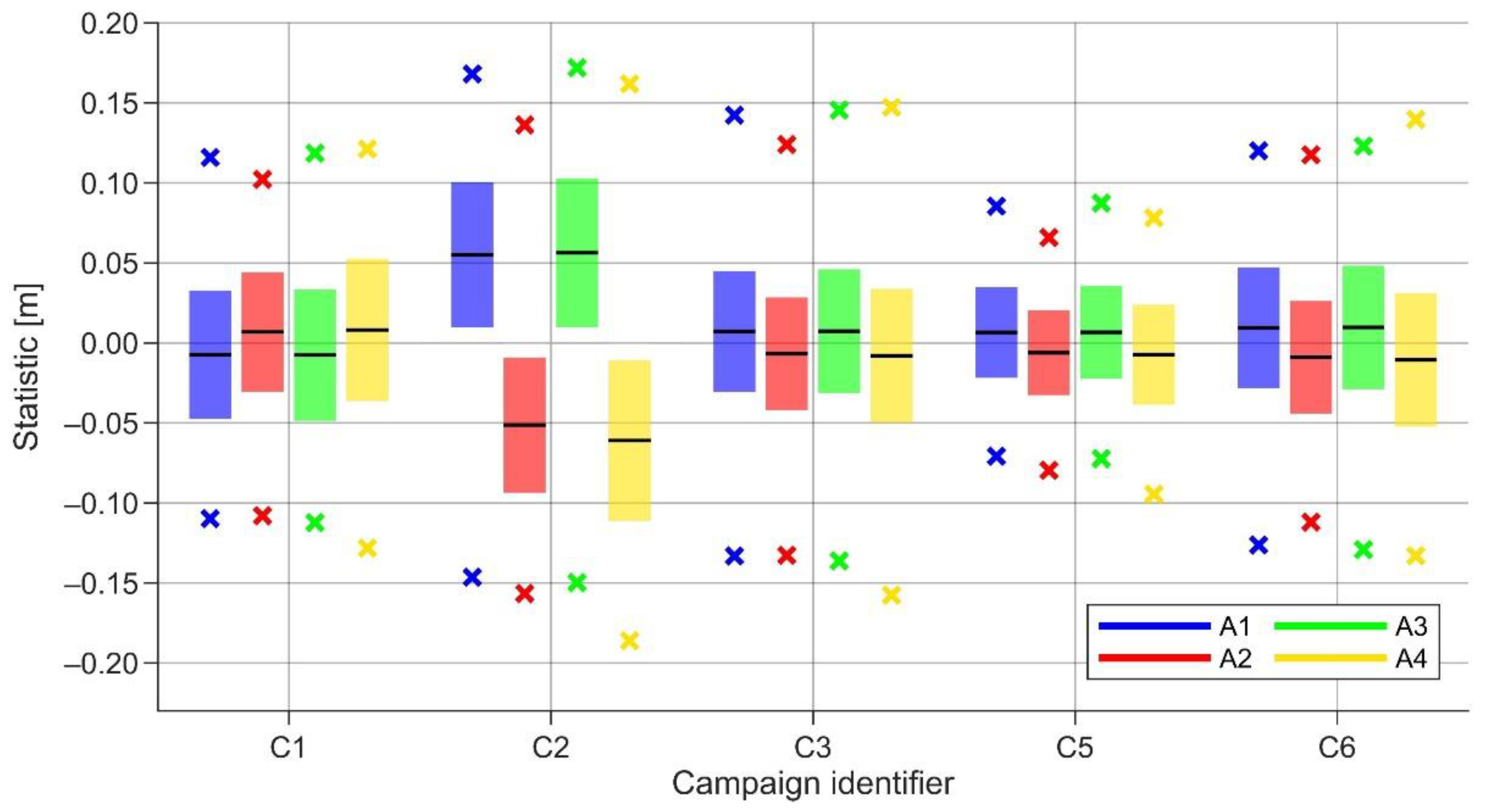
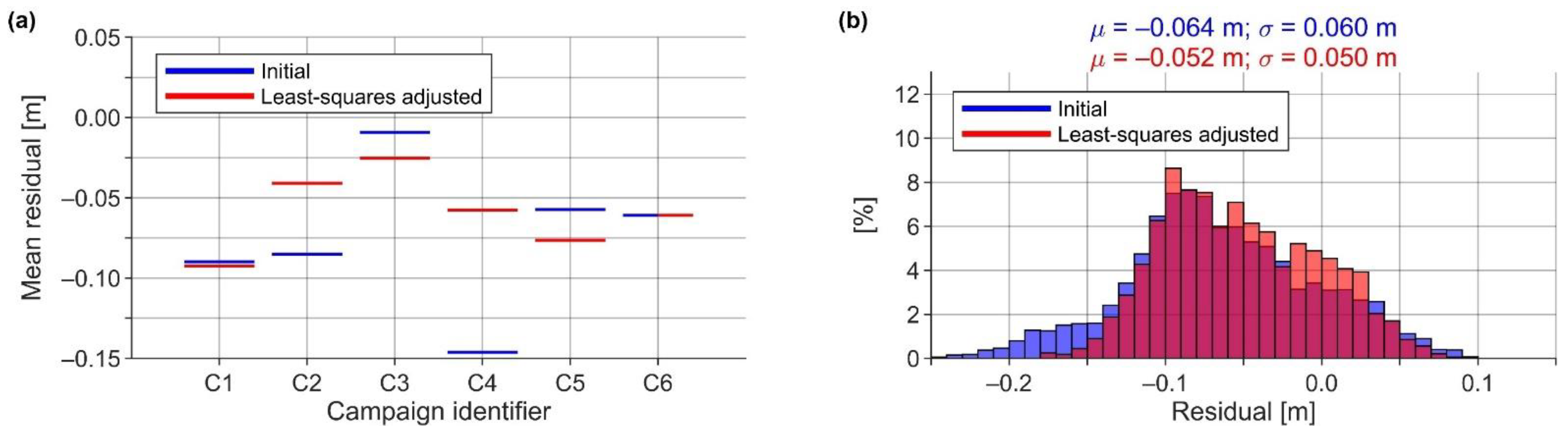
5.4. Validation and Least-Squares Adjustment of the Results

Ideally, the filtered and corrected residuals should be near-zero. However, such idealistic results cannot be expected, due to errors in the total station, tape, GNSS, and TG measurements; estimated corrections’ inaccuracies; and deficiencies in the used VLM, HDM, and geoid models. For instance, an examination of the residuals’ statistical properties (Figure 14a) shows biases between the results of different campaigns (notice mean values). A likely explanation is errors in tape measurements conducted in the harbor, for reducing surveys’ GNSS results to the sea surface (cf. Equation (8)). Since such measurements are subjective (the surveyor had to assess the optimal measure from the moving sea surface) and the vessel swayed slightly during the measurements, the tape-determined values likely induce the most significant errors.

The residuals’ standard deviation estimates vary between 1.8 cm and 5.5 cm (Figure 14a), demonstrating, in general, the satisfactory performance of the results, especially considering the variety of different datasets combined. The highest standard deviation estimate describes the C4 campaign, which is expected, as only two GNSS antennas (instead of four) could be used for the $iSS{H}_{CoM}^{Final}$ solution (cf. Section 5.1). Thus, the vessel’s high-frequency attitude changes likely contaminated the solution. On the other hand, although the second half of campaign C1 was conducted in windy and wavy conditions (due to a rising storm; recall the discussion in Section 4.1), the resulting standard deviation estimate was only 2.8 cm, suggesting that the approach used could successfully eliminate the vessel’s high-frequency attitude changes and marine conditions’ influence on GNSS measurements.

Another principal measure is the consistency of the residuals, which were, hence, compared at the campaign–internal intersections, by defining two criteria: (i) distance between points less than 250 m, and (ii) time between intersections (also consecutive points) more than 30 min. The two criteria had to be true at the same time. According to the first criterion, nearby parallel routes could also yield an intersection (geoidal heights and DT remain relatively unchanged over short distances), to avoid a lack of detected intersections when no actual route crossings existed. Moreover, if a vessel stopped for more than 30 min (e.g., to collect water samples) and did not drift significantly (more than 250 m), the stopping was counted as an intersection (the low-pass filtering influence disappears with 30 min: 53 measurements × 30 s = 26.5 min). The resulting statistics (Figure 14b) indicate a good consistency, with generally near-zero mean differences, and standard deviation estimates varying between 1.8 cm and 3.4 cm. Notably, the NKG2015 geoid model errors do not affect these comparisons, since the model is static (i.e., not a time-dependent variable).

The defined criteria were further employed to compare residuals of different campaigns at their intersections, following the principles described above. Notice in Figure 15 that the absolute values of mean differences (sign difference is due to the subtraction order) and standard deviation estimates differ slightly, for example, if campaign C1 is compared to C2 and vice-versa. Since the algorithm searches intersections by moving along the validated campaign, the two tests may yield different points for comparisons, due to the second intersection search criterion (i.e., the algorithm moves along different routes, detecting different points based on the definitions). Generally, these assessments show a good agreement between the residuals of different campaigns, in terms of standard deviation. The most significant residual differences were detected between campaigns C2 and C3, resulting in standard deviation estimates of 4.4 cm and 5.0 cm. The compared intersections were primarily detected in the relatively shallow Väinameri (cf. Figure 2), which could imply errors in squat estimation, but Väinameri also has more than 300 islands and islets, which may have influenced the HDM-embedded DT modeling.

Similarly to Figure 14a, Figure 15 suggests biases in the data (notice mean values). As described earlier, errors in tape measurements likely contributed significantly to these estimates. Hence, to increase the consistency of the residuals (and reduce the potential influence of tape measurement errors), the bias differences between campaigns were estimated by free network least-squares adjustment:

$$\widehat{X}={\left(A^{T}PA\right)}^{-1}{A}^{T}PL,$$

(22)

where vector $L$ denotes the estimated residuals’ mean differences between campaigns at intersections (i.e., the mean values shown in Figure 15) and design matrix $A$ corresponding comparisons. Thus, a system of $[6!/\left(6-2\right)!]-4=26$ linear equations was compiled (order matters, due to the second intersection search criterion, and for 4 comparisons, no intersections were detected). Weights $P$ were assigned according to the number of detected intersections between campaigns (cf. Figure 15). The estimated bias corrections denoted by vector $\widehat{X}$ (consisting of 6 estimates, one for each campaign) were then subtracted from the filtered and corrected residuals. This approach resulted in least-squares adjusted residuals, denoted as $r_{CoM}^{F+C+A}\left(\phi ,\lambda ,t\right)$ in the following.

Figure 16 presents the comparisons between the initial (filtered and corrected) and least-squares adjusted residuals. Since free network adjustment was used, the average value of the six mean residual estimates (i.e., the average of the 6 values shown in Figure 16a) remained unchanged. It can be noticed that the mean residuals of campaigns agree better after adjustment (Figure 16a) and that the results are more consistent (histograms in Figure 16b combine residuals of all six campaigns). However, since some biases still exist (which cannot be detected due to lack of intersections), the combined data standard deviation in Figure 16b exceeds that of most individual campaigns in Figure 14a.

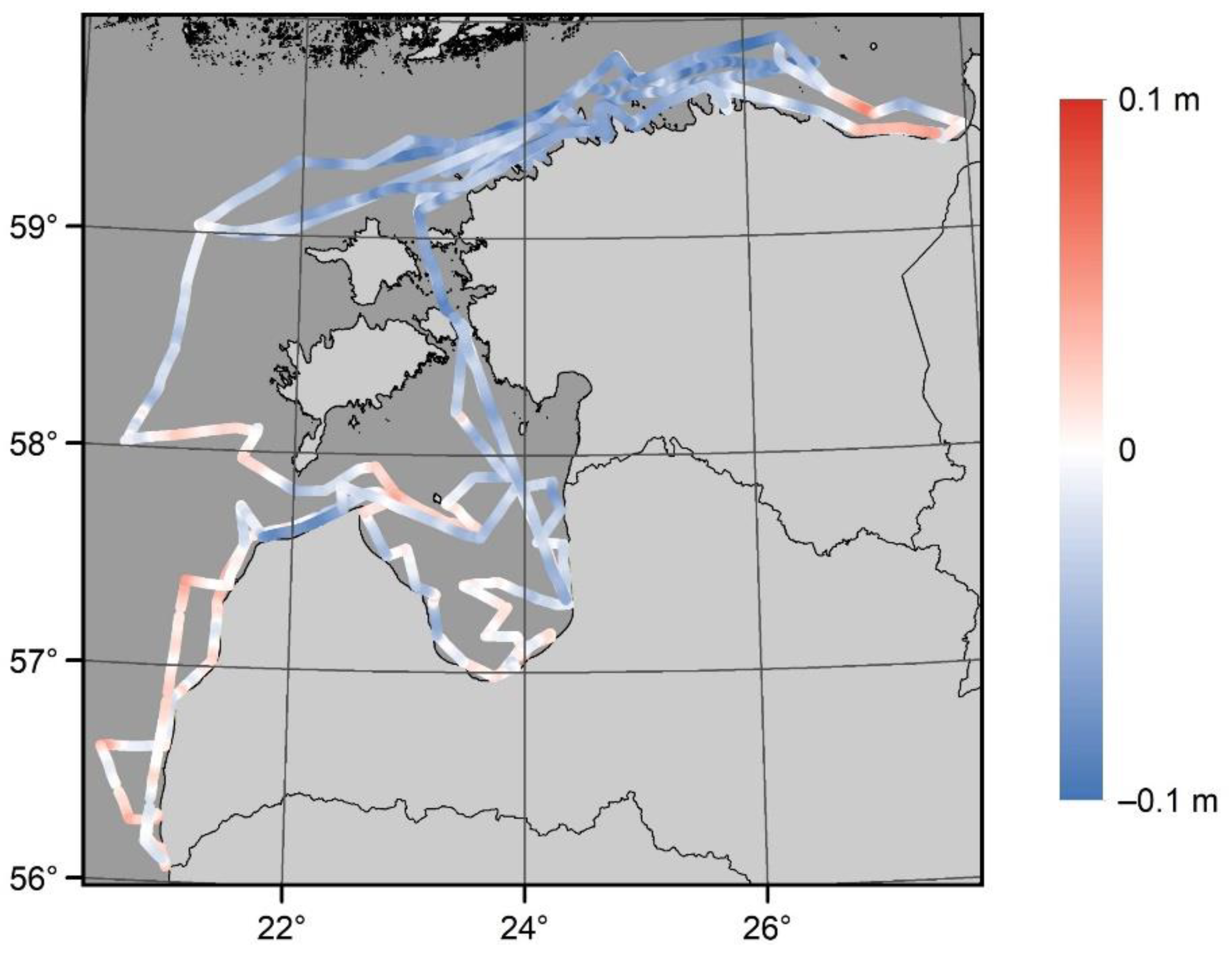
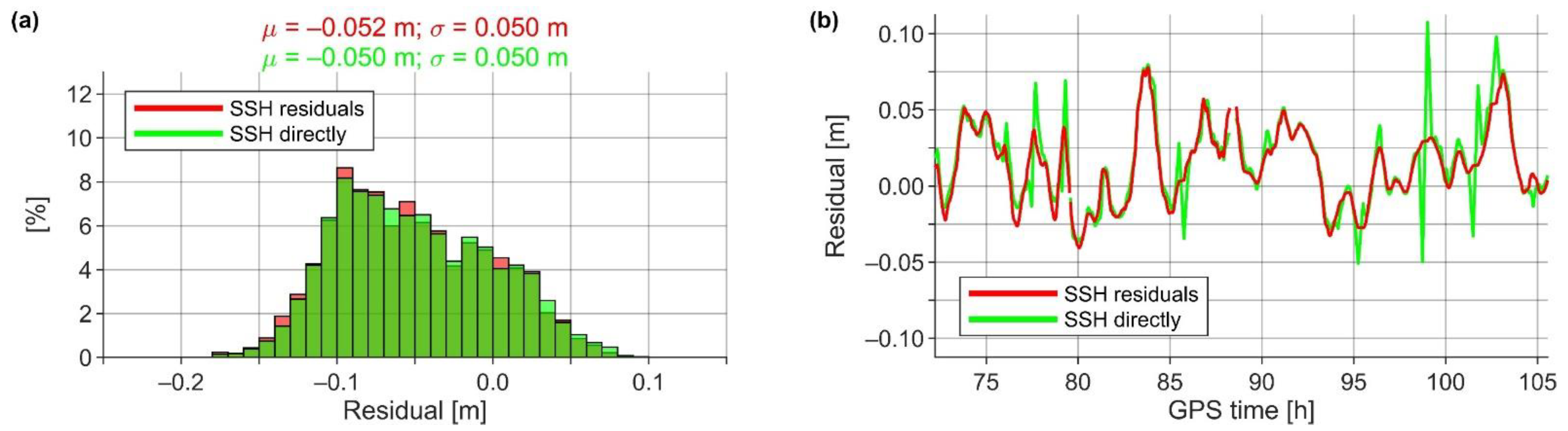
5.4.1. The Final Data Processing Results

The results in Figure 16b suggest that around a 5 cm accuracy can be achieved with the presented methodology, but it is also evident that a data bias of 5.2 cm exists simultaneously. According to Figure 17, the bias primarily originates from areas in the Gulf of Finland and Väinameri (refer to Figure 2) and appears to possess a long-wavelength nature. The bias could likely represent the NKG2015 geoid model errors to some extent. Similarly probable is that there are errors in the estimated DT, since even after correcting the used HDM with TG data, the determination of instantaneous DT with an accuracy of a few centimeters is a difficult task. It could also be that the tape measurements were systematically conducted in a way that resulted in lower than actual SSH. Unfortunately, these are all assumptions, and the origin of the bias currently remains unknown.

However, recall that this study aimed to derive accurate SSH from shipborne GNSS surveys. As a final step, the SSH was restored from filtered, corrected, and adjusted residuals (Equation (6) modification):

$$SS{H}_{CoM}^{F+C+A}\left(\phi ,\lambda ,t\right)=r_{CoM}^{F+C+A}\left(\phi ,\lambda ,t\right)+\widehat{DT}\left(\phi ,\lambda ,t\right)+\left[N\left(\phi ,\lambda ,t_0\right)+GC\left(\phi ,\lambda \right)·\left(t-t_0\right)\right],$$

(23)

where $\widehat{DT}$ and $N$ are correspondingly the DT and NKG2015 geoidal heights initially used to reduce SSH into residuals. The geoid change denoted as $GC$ is restored to obtain the actual SSH (recall that Equation (7) initially eliminated geoid change for data consistency). Assuming minimal error propagation during data filtering, the derived SSH should be mostly free of DT and geoid model errors. It is, thus, plausible that the expected accuracy of the derived SSH exceeds that of the presented and discussed residual values. Therefore, the derived SSH data are suitable for subsequent applications, such as validation of various marine models and measurements (with a limiting factor that measurements must be conducted at the same time as marine survey campaigns). Notably, the presented methodology works under harsh weather conditions (recall that the second half of the C1 campaign was conducted in stormy conditions), which is often the case in real life when marine campaigns are planned long in advance (i.e., the weather becomes unpredictable).

6. Discussion

This paper has described a methodology for deriving accurate SSH from the initial untreated post-processed shipborne GNSS measurements (detailed in [23]). The results indicate a 4.1 cm height determination accuracy, in terms of standard deviation (cf. Section 5.1), for the unfiltered SSH data. Since sea state conditions should not influence this estimate (i.e., the estimate represents a rigid system), it can also describe the final SSH accuracy, assuming sufficiently well-estimated vessel sailing-related corrections (cf. Section 5.3). Note that the application of the low-pass filter may have improved the accuracy by reducing data noise. Further data validation demonstrated standard deviation estimates of 1.8 cm to 5.5 cm for the determined residual values of individual campaigns (cf. Figure 14a), whereby the combination of all campaigns provided an estimate of 5.0 cm (cf. Figure 16b). The standard deviation estimates of campaign–internal intersections varied between 1.8 cm and 3.4 cm (cf. Figure 14b). By comparing the residuals of various campaigns to each other at intersections, the standard deviation estimates also remained within 5 cm (cf. Figure 15).

These results suggest that the developed methodology can provide at least a 5 cm accuracy for the SSH. For comparison, Baltic Sea region geoid validation studies (using NKG2015 model) have indicated the following agreement (in terms of standard deviation) with shipborne GNSS measurements: 3.4 cm [11], 3.8–6.8 cm [12], 4.2–12.0 cm [24], and 1.2–27.9 cm [32]. Other previous studies that investigated shipborne GNSS-determined SSH demonstrated 5–15 cm [10], 4.0–5.3 cm [33], and 7.4–11.9 cm [38] accuracies, in terms of standard deviation. The results of this study are, hence, in good agreement with the previous results, or surpass them.

Another notable result is that all GNSS data collection was autonomous [23], implying that GNSS devices can be installed on various vessels and for extended periods. Here, CORS-based post-processing of GNSS data were primarily used, but distant offshore locations may similarly be of interest for SSH measurements. It has been demonstrated in earlier studies that, for instance, the CSRS-PPP approach can provide reasonable height determination accuracy on such occasions, and even for transoceanic scenarios [24,37,38]. In future studies, it could be interesting to investigate the potential of the developed method exactly in distant offshore locations (using, e.g., CSRS-PPP instead of relying on CORS-based post-processing). This could provide essential SSH datasets with satisfactory accuracy for marine-related studies.

As is evident from the previous analyses and discussions, the presented joint SSH derivation and validation entails several steps and datasets that can influence the results. The following sections now examine the impact of some of these components. For that purpose, a single step or dataset was exchanged for an alternative, whereby all other data processing was conducted as described above.

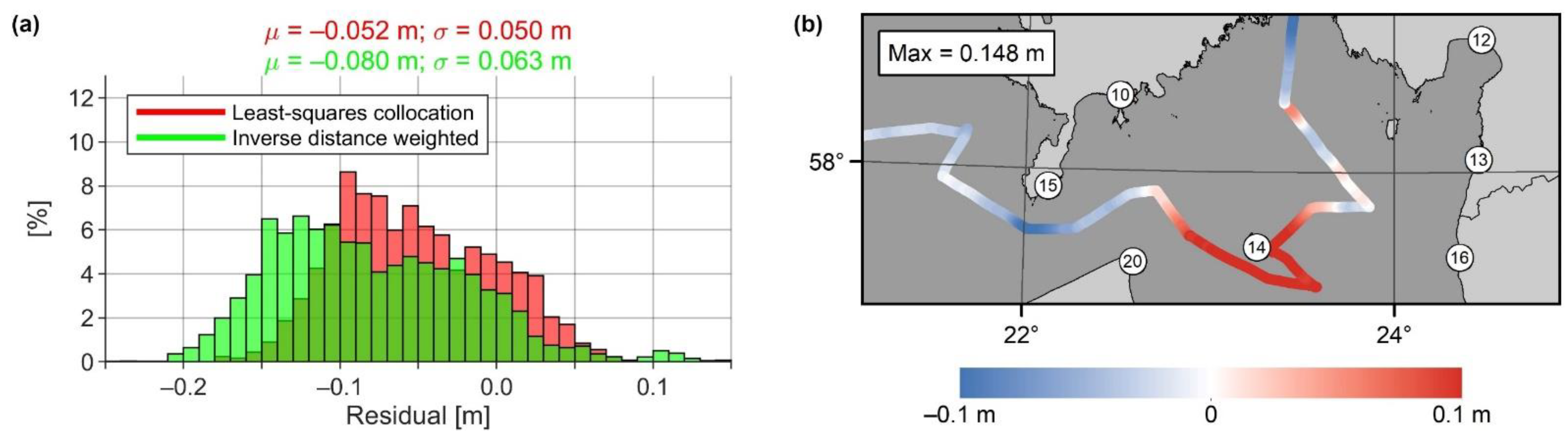
6.1. Dynamic Bias Prediction Method

Previously, refs. [15,30] used exact interpolators to predict offshore DB (required for correcting the used HDM for DT determination). Such an approach inherently assumes that there are no errors in the TG data and TGs connections to the height system(s), as well as that the estimated DB at a TG station is an expected value for all nearby offshore locations. In Section 4.1, it was suggested that this might not be the case. Therefore, a new approach was developed for estimating DB uncertainties and predicting offshore DB with an inexact interpolator (least-squares collocation) employing these estimates. The difference between an exact and inexact interpolator is now investigated.

A well-performing inverse distance weighted interpolation method (out of various exact interpolators, this one appears to provide the best results—Jahanmard, V., personal communication, September 2021) was used to predict offshore DB. A comparison with the developed approach is presented in Figure 18a. Notice that the residuals of the inverse distance weighted method are more spread out and biased; thus, highlighting the significant impact of the DB prediction approach on the results. Since the developed approach does not require the predicted DB to follow estimates at the locations of TG stations, the differences between the two histograms are primarily the direct impact of potentially erroneous (or misleading, since DT at TG stations may not represent offshore conditions) TG data.

Figure 18b presents residuals of the C2 campaign, derived using inverse distance weighted interpolation to predict offshore DB. Notice the residuals over a decimeter near TG₁₄, whereas no such residuals appeared when the newly developed method was used (cf. Figure 17). This difference is a direct cause of the issue described in Section 4.1, where the estimated DB at TG₁₄ was significantly higher (more than usual) than at the neighboring TG stations, likely due to offshore-directed strong winds, which may have pushed the water away from the harbor (i.e., lower TG readings result in higher DB, cf. Equation (3)).

An alternative example from Section 4.1 can also be further discussed. Namely, a significant contributor to the more negative bias of the inverse distance weighted method in Figure 18a is TG₄. It was demonstrated in [23], how the DT at TG₄ was up to 8–9 cm higher in comparison to the vessel’s nearby harbor (higher DT results in lower residual values, cf. Equation (2)). Relatedly, differences around a decimeter appeared for campaigns C2 and C3 near TG₄, between the inverse distance weighted method and the developed approach. These examples show how near-TG localized phenomena propagate to the estimated offshore DB with exact interpolators and demonstrate the superior performance of the developed approach.

6.2. Data Filtering Approach

In the production of SSH data, it would be convenient to skip the data validation step (as it requires derivation of DT), which means direct filtering of SSH data. However, in Section 2, it was suggested that gradients of DT and geoid might contaminate the low-pass filtering results. The Equation (20) low-pass filter was, hence, applied directly to the SSH data, to test this assumption. Subsequently, the filtered SSH data were reduced to residual values by the Equation (2) principle, and all following data processing was conducted as described in Section 5. The results were then compared to the initially derived residual values (Figure 19a). From this comparison, the directly filtered SSH resulted in slightly less biased residuals, whereby the variation of the residuals appears statistically insignificant. However, Figure 19b shows (an example from campaign C3) the actual impact of gradients on the filtering results (notice the peaks in the results when SSH was filtered directly).

The comparison in Figure 19b demonstrates the necessity of reducing the SSH to residual values before data filtering. Otherwise, gradients of DT and geoid may result in avoidable discrepancies of over 5 cm (the primary contributor being the geoid). An alternative could be to increase the GNSS data sampling rate, which would allow a shorter filtering window (spatial) length (cf. Figure 10), since a lengthy window causes such error propagation. Nevertheless, in steeper gradient areas, this may not be sufficient to avoid errors shown in Figure 19b. At the very least, geoidal heights should be reduced from SSH before data filtering, since the gradients of the geoid contribute the most to the described errors. Furthermore, note that the squat estimation was unsuccessful from SSH data directly, resulting in nearly twice as low squat estimates, meaning more negatively biased results (for the experiment in this section, the squat correction was applied as described in Section 5.3).

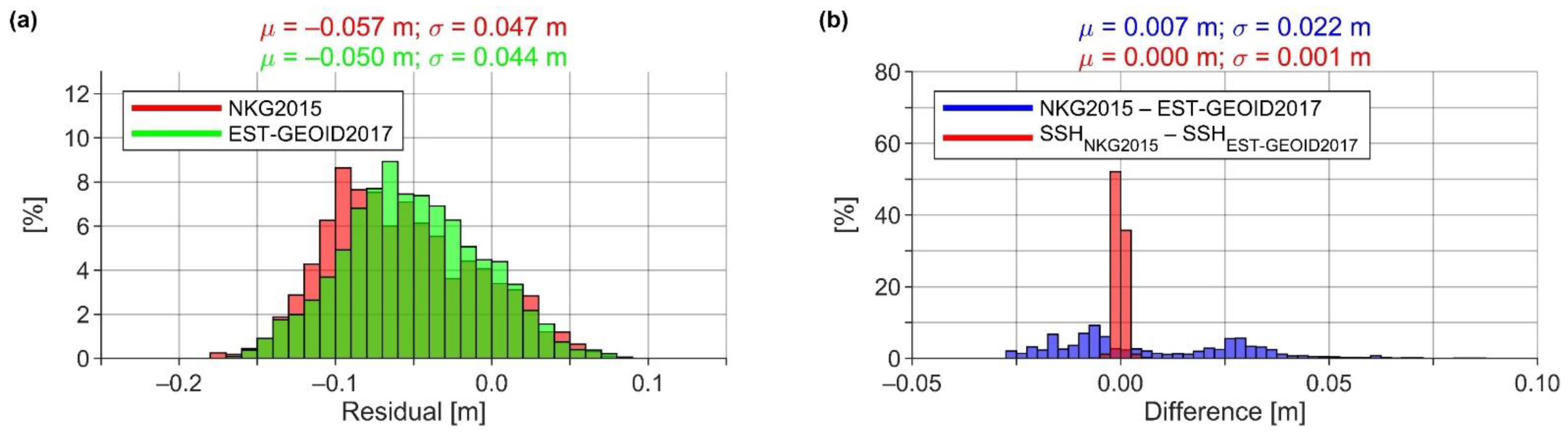
6.3. Choice of a Geoid Model

The accuracy of marine geoid models is often unknown, as the conventionally used precise GNSS-leveling control points cannot be used for validation purposes over marine areas. It can be assumed that the deficiencies in models may reach up to a few decimeters in the shorter wavelength spectrum. For instance, [11] and [15] showed errors over a decimeter in a marine gravity data void area in the NKG2015 geoid model (in the eastern Gulf of Finland, cf. Figure 2). In contrast, the Estonian national geoid model EST-GEOID2017 [58] appears to perform better, due to additional marine gravity data being included in the model development (see [11], who also provide a comprehensive review of these two models and their differences). The differences between the two models along the vessel’s routes are shown in Figure 20b.

For the next experiment, the NKG2015 geoid model was exchanged for the EST-GEOID2017 during data processing. The resulting discrepancies are compared in Figure 20a. Note that the red histogram differs from those in Figure 16b, Figure 18a, and Figure 19a, since the comparison was conducted over a reduced area (EST-GEOID2017 does not extend southward from 57° N). The comparison in Figure 20a demonstrates the slightly better performance of the EST-GEOID2017 model, which is consistent with previous studies’ results.

Since the geoid models contain errors, it would be interesting to know how model errors influence the resulting SSH data. This question can be investigated, as differences exist between the two used geoid models. Figure 20b suggests that the data filtering error propagation is negligible (as assumed in Section 5.4.1), because the two SSH datasets are practically the same. This finding indicates that if a geoid model has reasonable accuracy, the model’s inaccuracies do not influence the derived SSH (by reducing SSH to residuals for data filtering), which also implies that errors in DT do not propagate significantly either. The results would likely be poorer by neglecting geoid and DT information entirely during data processing (recall the example in Section 6.2).

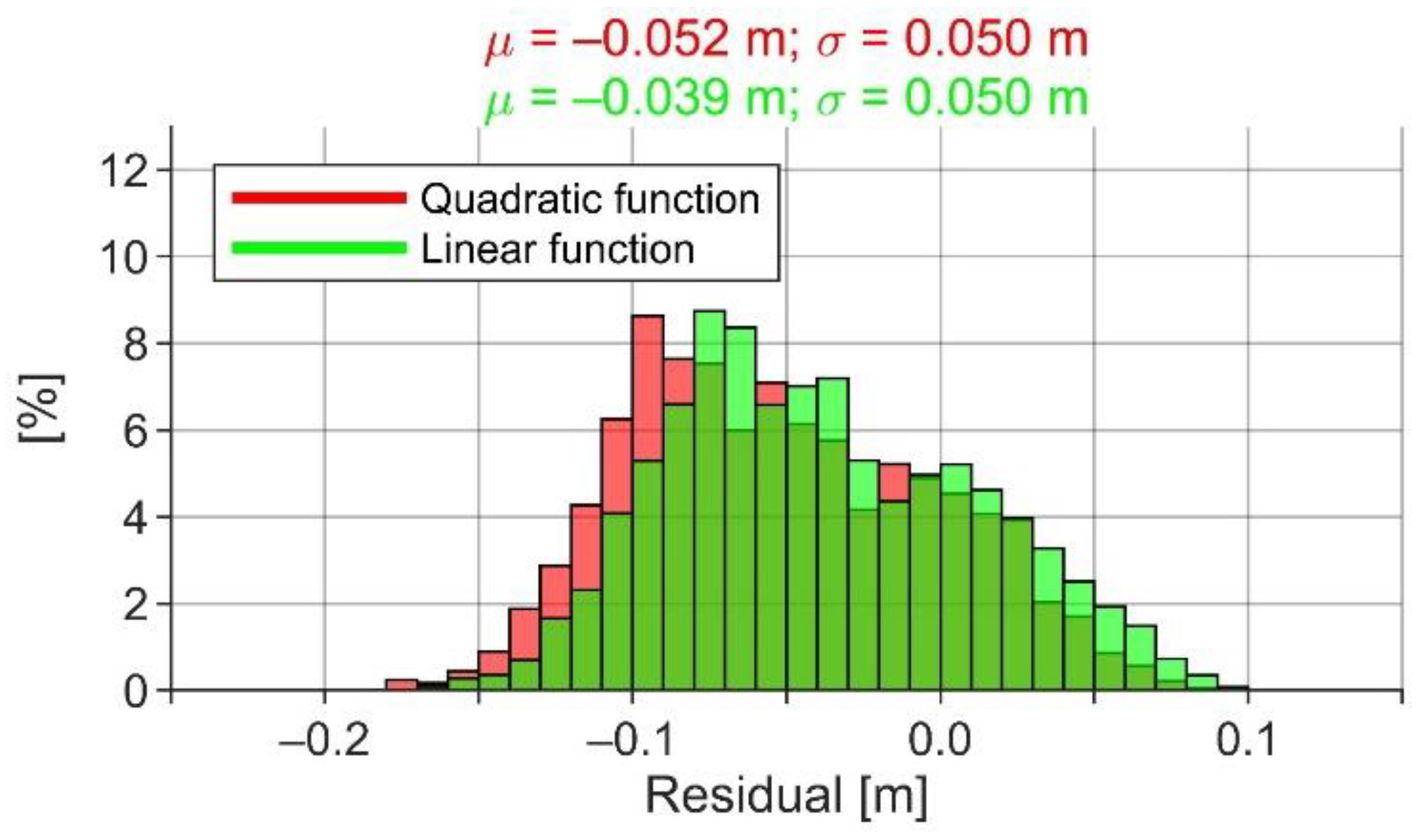
6.4. Squat Estimation Function

Ideally, squat information should be provided by a vessel-specific squat table. Such a table was not available for this study. Thus, the squat correction was estimated empirically as a direct data derivative (cf. Section 5.3). Since the squat is approximately a quadratic velocity function, a quadratic function was fitted to the empirical data in the least-squares sense. As an alternative, a least-squares fit of a linear function was also used to approximate squat correction (cf. Figure 13a). The resulting residuals from using these two functions are compared in Figure 21. Note that the offset term was not considered for the linear function, as was the case with the quadratic function (cf. Equation (21)).

Although the use of the quadratic function is, in theory, more correct, the results in Figure 21 indicate a better performance for the linear function, as the residuals are significantly less biased toward negative. It, thus, appears that the quadratic function underestimates the squat correction. The result also implies that a portion of the 5.2 cm bias in the data originates from inaccurate squat correction.

7. Conclusions

This contribution presented a methodology for deriving accurate SSH from initial untreated post-processed GNSS data. The methodology involves a joint validation of the results using a geoid model and realistic DT to reduce SSH to residual values. Since GNSS measurements should be low-pass filtered to eliminate the effect of sea state conditions, the approach can also enhance SSH data accuracy, by avoiding error propagation due to DT and geoid gradients, which in this study could have caused larger than 5 cm errors. Furthermore, a rigid system of four GNSS antennas was used to eliminate the vessel’s high-frequency attitude changes from the measurement data. Such a system is also beneficial, as it can be validated internally. Accordingly, the results indicated a 4.1 cm height determination accuracy for the whole SSH dataset. Other data validation (e.g., examination of residual values and intersection analyses) results ranged from 1.8 cm to 5.5 cm, in terms of standard deviation; suggesting that SSH can be determined with an accuracy of around 5 cm using the shipborne GNSS method.

As mentioned, the validation requires DT information. A new method was developed that combines the properties of TG data and an HDM. Tide gauge data allow estimating the spatiotemporal bias of an HDM; thus, linking it to used vertical datum (e.g., a novel geoid-based Baltic Sea Chart Datum 2000), whereby the qualities of spatiotemporal bias are used to constrain TG data errors. As a result, realistic DT relative to an equipotential surface can be obtained, which could be beneficial in oceanographic research for studying marine processes accurately (e.g., determination of mean DT relative to an equipotential surface for studying currents). According to the SSH residual value validations, the developed approach was demonstrated to surpass the one used by [15,30], with an improvement in standard deviation estimate from 6.3 cm to 5.0 cm, and mean residual from −8.0 cm to −5.2 cm.

References

1. Visser, H.; Dangendorf, S.; Petersen, A.C. A review of trend models applied to sea level data with reference to the “acceleration-deceleration debate”. J. Geophys. Res. Ocean. 2015, 120, 3873–3895. [Google Scholar] [CrossRef]
2. Breili, K.; Simpson, M.J.R.; Nilsen, J.E.Ø. Observed sea-level changes along the Norwegian coast. J. Mar. Sci. Eng. 2017, 5, 29. [Google Scholar] [CrossRef] [Green Version]
3. Madsen, K.S.; Høyer, J.L.; Suursaar, Ü.; She, J.; Knudsen, P. Sea level trends and variability of the Baltic Sea from 2D statistical reconstruction and altimetry. Front. Earth Sci. 2019, 7, 243. [Google Scholar] [CrossRef]
4. Vu, P.L.; Frappart, F.; Darrozes, J.; Marieu, V.; Blarel, F.; Ramillien, G.; Bonnefond, P.; Birol, F. Multi-satellite altimeter validation along the French Atlantic coast in the southern Bay of Biscay from ERS-2 to SARAL. Remote Sens. 2018, 10, 93. [Google Scholar] [CrossRef] [Green Version]
5. Yang, J.; Zhang, J.; Wang, C. Sentinel-3A SRAL global statistical assessment and cross-calibration with Jason-3. Remote Sens. 2019, 11, 1573. [Google Scholar] [CrossRef] [Green Version]
6. Liibusk, A.; Kall, T.; Rikka, S.; Uiboupin, R.; Suursaar, Ü.; Tseng, K.-H. Validation of Copernicus sea level altimetry products in the Baltic Sea and Estonian lakes. Remote Sens. 2020, 12, 4062. [Google Scholar] [CrossRef]
7. Passaro, M.; Cipollini, P.; Vignudelli, S.; Quartly, G.D.; Snaith, H.M. ALES: A multi-mission adaptive subwaveform retracker for coastal and open ocean altimetry. Remote Sens. Environ. 2014, 145, 173–189. [Google Scholar] [CrossRef] [Green Version]
8. Cipollini, P.; Calafat, F.M.; Jevrejeva, S.; Melet, A.; Prandi, P. Monitoring sea level in the coastal zone with satellite altimetry and tide gauges. Surv. Geophys. 2017, 38, 33–57. [Google Scholar] [CrossRef] [Green Version]
9. Vignudelli, S.; Birol, F.; Benveniste, J.; Fu, L.-L.; Picot, N.; Raynal, M.; Roinard, H. Satellite altimetry measurements of sea level in the coastal zone. Surv. Geophys. 2019, 40, 1319–1349. [Google Scholar] [CrossRef]
10. Bouin, M.-N.; Ballu, V.; Calmant, S.; Boré, J.-M.; Folcher, E.; Ammann, J. A kinematic GPS methodology for sea surface mapping, Vanuatu. J. Geod. 2009, 83, 1203. [Google Scholar] [CrossRef]
11. Varbla, S.; Ellmann, A.; Delpeche-Ellmann, N. Validation of marine geoid models by utilizing hydrodynamic model and shipborne GNSS profiles. Mar. Geod. 2020, 43, 134–162. [Google Scholar] [CrossRef]
12. Saari, T.; Bilker-Koivula, M.; Koivula, H.; Nordman, M.; Häkli, P.; Lahtinen, S. Validating geoid models with marine GNSS measurements, sea surface models, and additional gravity observations in the Gulf of Finland. Mar. Geod. 2021, 44, 196–214. [Google Scholar] [CrossRef]
13. Gruno, A.; Liibusk, A.; Ellmann, A.; Oja, T.; Vain, A.; Jürgenson, H. Determining sea surface heights using small footprint airborne laser scanning. In Proceedings of the Remote Sensing of the Ocean, Sea Ice, Coastal Waters, and Large Water Regions 2013, Dresden, Germany, 23–26 September 2013. [Google Scholar] [CrossRef]
14. Zlinszky, A.; Timár, G.; Weber, R.; Székely, B.; Briese, C.; Ressl, C.; Pfeifer, N. Observation of a local gravity potential isosurface by airborne lidar of Lake Balaton, Hungary. Solid Earth 2014, 5, 355–369. [Google Scholar] [CrossRef] [Green Version]
15. Varbla, S.; Ellmann, A.; Delpeche-Ellmann, N. Applications of airborne laser scanning for determining marine geoid and surface waves properties. Eur. J. Remote Sens. 2021, 54, 557–567. [Google Scholar] [CrossRef]
16. Xu, X.-Y.; Xu, K.; Shen, H.; Liu, Y.-L.; Liu, H.-G. Sea surface height and significant wave height calibration methodology by a GNSS buoy campaign for HY-2A altimeter. IEEE J. Sel. Top. Appl. Earth Obs. Remote Sens. 2016, 9, 5252–5261. [Google Scholar] [CrossRef]
17. Zhou, B.; Watson, C.; Legresy, B.; King, M.A.; Beardsley, J.; Deane, A. GNSS/INS-equipped buoys for altimetry validation: Lessons learnt and new directions from the Bass Strait validation facility. Remote Sens. 2020, 12, 3001. [Google Scholar] [CrossRef]
18. Penna, N.T.; Morales Maqueda, M.A.; Martin, I.; Guo, J.; Foden, P.R. Sea surface height measurement using a GNSS wave glider. Geophys. Res. Lett. 2018, 45, 5609–5616. [Google Scholar] [CrossRef]
19. Chupin, C.; Ballu, V.; Testut, L.; Tranchant, Y.-T.; Calzas, M.; Poirier, E.; Coulombier, T.; Laurain, O.; Bonnefond, P.; Team FOAM Project. Mapping sea surface height using new concepts of kinematic GNSS instruments. Remote Sens. 2020, 12, 2656. [Google Scholar] [CrossRef]
20. Rocken, C.; Johnson, J.; Van Hove, T.; Iwabuchi, T. Atmospheric water vapor and geoid measurements in the open ocean with GPS. Geophys. Res. Lett. 2005, 32, L12813. [Google Scholar] [CrossRef] [Green Version]
21. Jürgenson, H.; Liibusk, A.; Ellmann, A. Geoid profiles in the Baltic Sea determined using GPS and sea level surface. Geod. Cartogr. 2008, 34, 109–115. [Google Scholar] [CrossRef] [Green Version]
22. Ince, E.S.; Förste, C.; Barthelmes, F.; Pflug, H.; Li, M.; Kaminskis, J.; Neumayer, K.-H.; Michalak, G. Gravity measurements along commercial ferry lines in the Baltic Sea and their use for geodetic purposes. Mar. Geod. 2020, 43, 573–602. [Google Scholar] [CrossRef]
23. Liibusk, A.; Varbla, S.; Ellmann, A.; Vahter, K.; Uiboupin, R.; Delpeche-Ellmann, N. Shipborne GNSS acquisition of sea surface heights in the Baltic Sea. J. Geod. Sci. 2022, in print. [CrossRef]
24. Varbla, S.; Ellmann, A.; Märdla, S.; Gruno, A. Assessment of marine geoid models by ship-borne GNSS profiles. Geod. Cartogr. 2017, 43, 41–49. [Google Scholar] [CrossRef] [Green Version]
25. Schwabe, J.; Ågren, J.; Liebsch, G.; Westfeld, P.; Hammarklint, T.; Mononen, J.; Andersen, O.B. The Baltic Sea Chart Datum 2000 (BSCD2000)—Implementation of a common reference level in the Baltic Sea. Int. Hydrogr. Rev. 2020, 23, 63–83. [Google Scholar]
26. Varbla, S.; Ågren, J.; Ellmann, A.; Poutanen, M. Treatment of tide gauge time series and marine GNSS measurements for vertical land motion with relevance to the implementation of the Baltic Sea Chart Datum 2000. Remote Sens. 2022, 14, 920. [Google Scholar] [CrossRef]
27. Suursaar, Ü.; Kall, T. Decomposition of relative sea level variations at tide gauges using results from four Estonian precise levelings and uplift models. IEEE J. Sel. Top. Appl. Earth Obs. Remote Sens. 2018, 11, 1966–1974. [Google Scholar] [CrossRef]
28. Kollo, K.; Ellmann, A. Geodetic reconciliation of tide gauge network in Estonia. Geophysica 2019, 54, 27–38. [Google Scholar]
29. Lagemaa, P.; Elken, J.; Kõuts, T. Operational sea level forecasting in Estonia. Est. J. Eng. 2011, 17, 301–331. [Google Scholar] [CrossRef] [Green Version]
30. Jahanmard, V.; Delpeche-Ellmann, N.; Ellmann, A. Realistic dynamic topography through coupling geoid and hydrodynamic models of the Baltic Sea. Cont. Shelf Res. 2021, 222, 104421. [Google Scholar] [CrossRef]
31. Slobbe, D.C.; Verlaan, M.; Klees, R.; Gerritsen, H. Obtaining instantaneous water levels relative to a geoid with a 2D storm surge model. Cont. Shelf Res. 2013, 52, 172–189. [Google Scholar] [CrossRef]
32. Nordman, M.; Kuokkanen, J.; Bilker-Koivula, M.; Koivula, H.; Häkli, P.; Lahtinen, S. Geoid validation on the Baltic Sea using ship-borne GNSS data. Mar. Geod. 2018, 41, 457–476. [Google Scholar] [CrossRef]
33. Roggenbuck, O.; Reinking, J. Sea surface heights retrieval from ship-based measurements assisted by GNSS signal reflections. Mar. Geod. 2019, 42, 1–24. [Google Scholar] [CrossRef]
34. Metsar, J.; Kollo, K.; Ellmann, A. Modernization of the Estonian national GNSS reference station network. Geod. Cartogr. 2018, 44, 55–62. [Google Scholar] [CrossRef] [Green Version]
35. Balodis, J.; Morozova, K.; Reiniks, M.; Normand, M. Normal heights for GNSS reference station antennas. In Proceedings of the IOP Conference Series: Materials Science and Engineering, Riga, Latvia, 27–29 September 2017. [Google Scholar] [CrossRef]
36. Vestøl, O.; Ågren, J.; Steffen, H.; Kierulf, H.; Tarasov, L. NKG2016LU: A new land uplift model for Fennoscandia and the Baltic region. J. Geod. 2019, 93, 1759–1779. [Google Scholar] [CrossRef] [Green Version]
37. Roggenbuck, O.; Reinking, J.; Härting, A. Oceanwide precise determination of sea surface height from in-situ measurements on cargo ships. Mar. Geod. 2014, 37, 77–96. [Google Scholar] [CrossRef]
38. Shih, H.-C.; Yeh, T.-K.; Du, Y.; He, K. Accuracy assessment of sea surface height measurement obtained from shipborne PPP positioning. J. Surv. Eng. 2021, 147, 04021022. [Google Scholar] [CrossRef]
39. Natural Resources Canada. Precise Point Positioning. Available online: https://webapp.geod.nrcan.gc.ca/geod/tools-outils/ppp.php (accessed on 28 February 2022).
40. Ågren, J.; Strykowski, G.; Bilker-Koivula, M.; Omang, O.; Märdla, S.; Forsberg, R.; Ellmann, A.; Oja, T.; Liepins, I.; Parseliunas, E.; et al. The NKG2015 gravimetric geoid model for the Nordic-Baltic region. In Proceedings of the International Symposium on Gravity, Geoid and Height Systems 2016, Thessaloniki, Greece, 19–23 September 2016. [Google Scholar] [CrossRef]
41. Poutanen, M.; Vermeer, M.; Mäkinen, J. The permanent tide in GPS positioning. J. Geod. 1996, 70, 499–504. [Google Scholar] [CrossRef]
42. Ihde, J.; Mäkinen, J.; Sacher, M. Conventions for the Definition and Realization of a European Vertical Reference System (EVRS); Version 5.2; Federal Agency for Cartography and Geodesy (BKG): Frankfurt, Germany, 2019.
43. Varbla, S.; Ellmann, A.; Delpeche-Ellmann, N. Utilizing airborne laser scanning and geoid model for near-coast improvements in sea surface height and marine dynamics. J. Coast. Res. 2020, 95, 1339–1343. [Google Scholar] [CrossRef]
44. Hordoir, R.; Axell, L.; Höglund, A.; Dieterich, C.; Fransner, F.; Gröger, M.; Liu, Y.; Pemberton, P.; Schimanke, S.; Andersson, H.; et al. Nemo-Nordic 1.0: A NEMO-based ocean model for the Baltic and North seas—Research and operational applications. Geosci. Model Dev. 2019, 12, 363–386. [Google Scholar] [CrossRef] [Green Version]
45. Kärnä, T.; Ljungemyr, P.; Falahat, S.; Ringgaard, I.; Axell, L.; Korabel, V.; Murawski, J.; Maljutenko, I.; Lindenthal, A.; JanDT-Scheelke, S.; et al. Nemo-Nordic 2.0: Operational marine forecast model for the Baltic Sea. Geosci. Model Dev. 2021, 14, 5731–5749. [Google Scholar] [CrossRef]
46. LVĢMC Hydrological Data Search (in Latvian). Available online: https://www.meteo.lv/hidrologija-datu-meklesana/?nid=466 (accessed on 28 February 2021).
47. SMHI Oceanographic Observations. Available online: https://www.smhi.se/data/oceanografi/ladda-ner-oceanografiska-observationer/#param=sealevelrh2000,stations=all (accessed on 28 February 2021).
48. FMI Observations. Available online: https://en.ilmatieteenlaitos.fi/download-observations#!/ (accessed on 28 February 2021).
49. EMODnet Data Explorer. Available online: http://www.emodnet-physics.eu/Map/DefaultMap.aspx (accessed on 28 February 2021).
50. LVĢMC Observation Network (in Latvian). Available online: https://www.meteo.lv/hidrologijas-staciju-karte/?nid=465 (accessed on 28 February 2021).
51. Theoretical Mean Water and Geodetical Height Systems in Finland. Available online: https://en.ilmatieteenlaitos.fi/theoretical-mean-sea-level (accessed on 28 February 2021).
52. EVRS Height Datum Relations. Available online: https://evrs.bkg.bund.de/Subsites/EVRS/EN/Projects/HeightDatumRel/height-datum-rel.html (accessed on 28 February 2021).
53. Lan, W.-H.; Kuo, C.-Y.; Kao, H.-C.; Lin, L.-C.; Shum, C.K.; Tseng, K.-H.; Chang, J.-C. Impact of geophysical and datum corrections on absolute sea-level trends from tide gauges around Taiwan, 1993–2015. Water 2017, 9, 480. [Google Scholar] [CrossRef]
54. Denys, P.H.; Beavan, R.J.; Hannah, J.; Pearson, C.F.; Palmer, N.; Denham, M.; Hreinsdottir, S. Sea level rise in New Zealand: The effect of vertical land motion on century-long tide gauge records in a tectonically active region. J. Geophys. Res. Solid Earth 2020, 125, e2019JB018055. [Google Scholar] [CrossRef]
55. Moritz, H. Advanced Physical Geodesy; Wichmann: Karlsruhe, Germany, 1980. [Google Scholar]
56. Kasper, J.F. A second-order Markov gravity anomaly model. J. Geophys. Res. 1971, 76, 7844–7849. [Google Scholar] [CrossRef]
57. Barrass, C.B. Ship Design and Performance for Masters and Mates; Elsevier: Oxford, UK, 2004. [Google Scholar]
58. Ellmann, A.; Märdla, S.; Oja, T. The 5 mm geoid model for Estonia computed by the least squares modified Stokes’s formula. Surv. Rev. 2020, 52, 352–372. [Google Scholar] [CrossRef]
Figure 1. Interrelations between the used datasets. The solid lines denote geometry at a reference epoch, whereby the dashed lines show the vertical land motion (VLM) affected geometry at a GNSS observation epoch. Global sea level rise and geoid change trends are neglected for simplification (i.e., the sea’s surface is assumed to be unchanged). Notice that the depicted dynamic bias (DB) is negative, cf. Equation (3).
Remotesensing 14 02368 g001
Figure 2. Study area (see the red rectangle) and routes of marine survey campaigns. Numbered circles denote the used TG stations, and red triangles continuously operating reference stations that were employed for GNSS post-processing. Colored background and grey isolines (contour interval is one meter) depict the NKG2015 quasigeoid model.
Remotesensing 14 02368 g002
Figure 3. Correlation coefficients between TG and HDM data at the TG locations (based on all 792 h of used data, cf. Table 1). For better readability, only the top of the vertical scale is shown.
Remotesensing 14 02368 g003
Figure 4. The mean predicted DB (left) and standard deviation estimates of predicted DB (right) for campaigns C1 (a,b), C2 (c,d), and C6 (e,f). The colored circles show, correspondingly, the mean DB values and standard deviation estimates of the DB values determined at the locations of TG stations.
Remotesensing 14 02368 g004
Figure 5. Uncertainty estimates of DB (a) at each TG station (refer to Figure 2) during the C1 campaign (i.e., σ D B ( t H ) ; cf. Equation (12)) and (b) averaged for all campaigns.
Remotesensing 14 02368 g005
Figure 6. The (a) predicted DB and (b) corrected HDM-based DT during marine survey campaigns.
Remotesensing 14 02368 g006
Figure 7. Pitch, roll, and yaw motions of a moving vessel and relative locations of the used GNSS antennas (colored blue). The red lines are the principal axes of the vessel, whereas the black lines denote total station measurement derived distances between antennas and imaginary (magenta colored) intersection points. All points are shown in horizontal projection (i.e., as reduced to the sea surface).
Remotesensing 14 02368 g007
Figure 8. Statistical properties of discrepancies d A ξ for antennas A1–A4. The black lines are mean values, and colored bars denote standard deviation estimates. Crosses show 99th percentile minimum and maximum discrepancies.
Remotesensing 14 02368 g008
Figure 9. Sum of absolute difference (SoAD) functions for the marine survey campaigns. Optimal filtering window sizes are shown with dashed vertical lines.
Remotesensing 14 02368 g009
Figure 10. Filtering window length dependency on GNSS sampling rate and vessel velocity, by assuming an optimal filtering window size of 53 measurements.
Remotesensing 14 02368 g010
Figure 11. Residuals of the C2 campaign for antennas A1–A4 and the mass center solution (denoted CoM), (a) before and (b) after low-pass filtering.
Remotesensing 14 02368 g011
Figure 12. Statistical properties of differences between unfiltered and filtered residuals (filtered results were subtracted from unfiltered) for antennas A1–A4 and the mass center solution (denoted CoM). The black lines are mean values, and colored bars denote standard deviation estimates. Crosses show 99th percentile minimum and maximum differences.
Remotesensing 14 02368 g012
Figure 13. Empirically estimated (a) squat and (b) static draft corrections.
Remotesensing 14 02368 g013
Figure 14. Statistical properties of (a) filtered and corrected residuals and (b) their differences at campaign–internal intersections. The black lines are mean values, and colored bars denote standard deviation estimates. With crosses are shown minimum and maximum residuals and their differences at intersections in (a,b), respectively.
Remotesensing 14 02368 g014
Figure 15. Statistical properties of filtered and corrected residuals’ differences at intersections between campaigns. The black lines are mean values, and colored bars denote standard deviation estimates. Crosses show minimum and maximum differences. Note that color shows the validated campaign and the X-axis validation dataset. In square brackets are the total number of detected intersections for each comparison.
Remotesensing 14 02368 g015
Figure 16. The (a) mean values of residuals (the initial ones coincide with those in Figure 14a) and (b) histograms of residuals (all campaigns combined).
Remotesensing 14 02368 g016
Figure 17. The final filtered, corrected, and least-squares adjusted residuals r C o M F + C + A .
Remotesensing 14 02368 g017
Figure 18. (a) Histograms of residuals (all campaigns combined): the impact of the DB prediction method, and (b) filtered, corrected, and least-squares adjusted residuals, derived using inverse distance weighted interpolation for DB prediction. Numbered circles in (b) denote the used TG stations.
Remotesensing 14 02368 g018
Figure 19. (a) Histograms of residuals (all campaigns combined): the impact of the data filtering approach, and (b) a comparison between residuals (a section of campaign C3) resulting from the two approaches.
Remotesensing 14 02368 g019
Figure 20. (a) Histograms of residuals (all campaigns combined): the impact of geoid model choice, and (b) histograms showing differences between the NKG2015 and EST-GEOID2017 models (along the vessel’s routes) and the SSH datasets derived using these models during data processing.
Remotesensing 14 02368 g020
Figure 21. Histograms of residuals (all campaigns combined): the impact of squat estimation function.
Remotesensing 14 02368 g021