
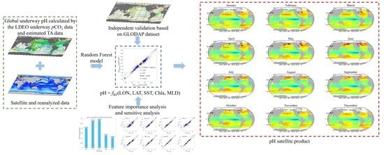
Remote Sensing of Global Sea Surface pH Based on Massive Underway Data and Machine Learning

 , and
, and
Abstract
:
1. Introduction
2. Data and Methods
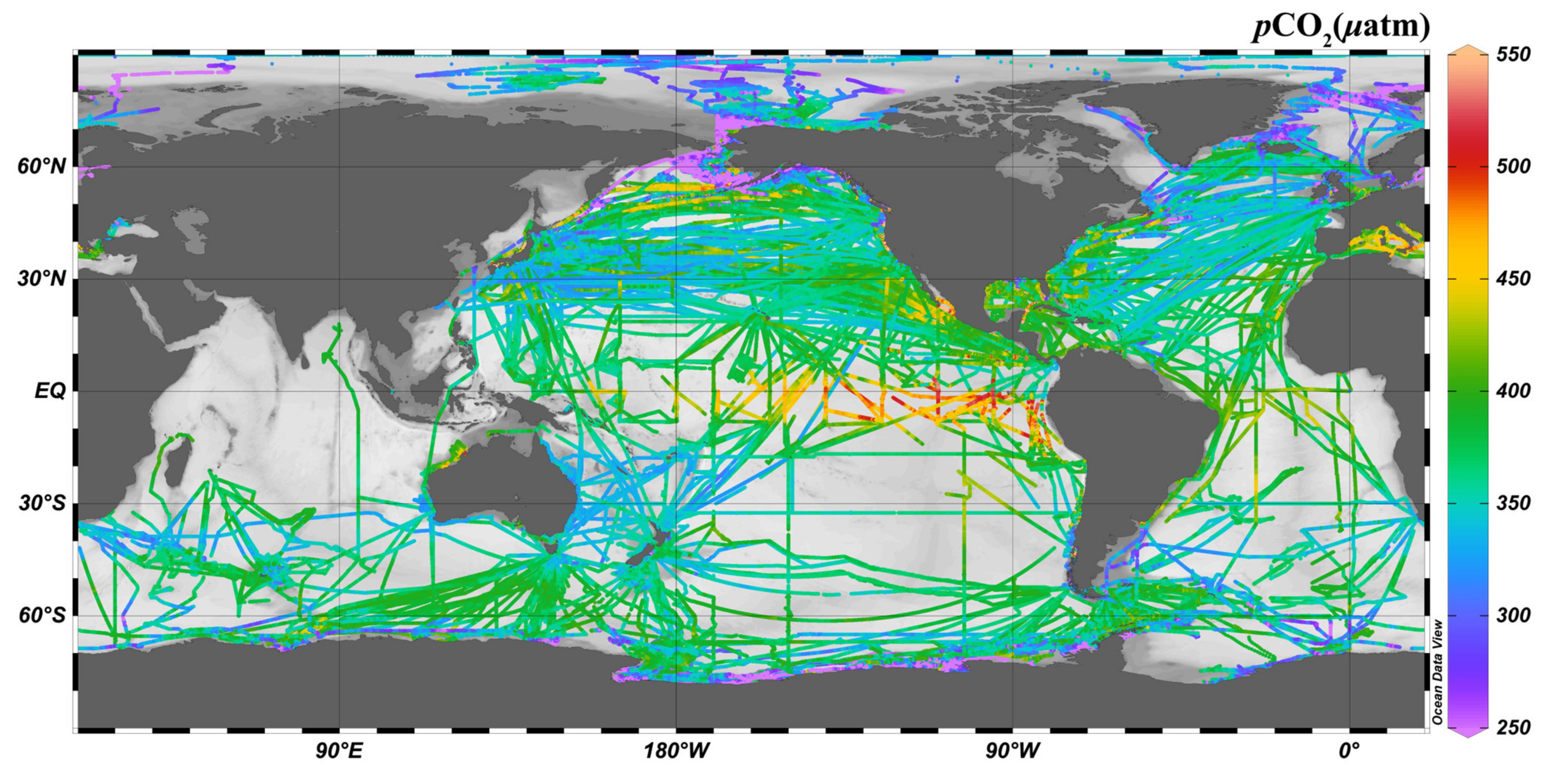
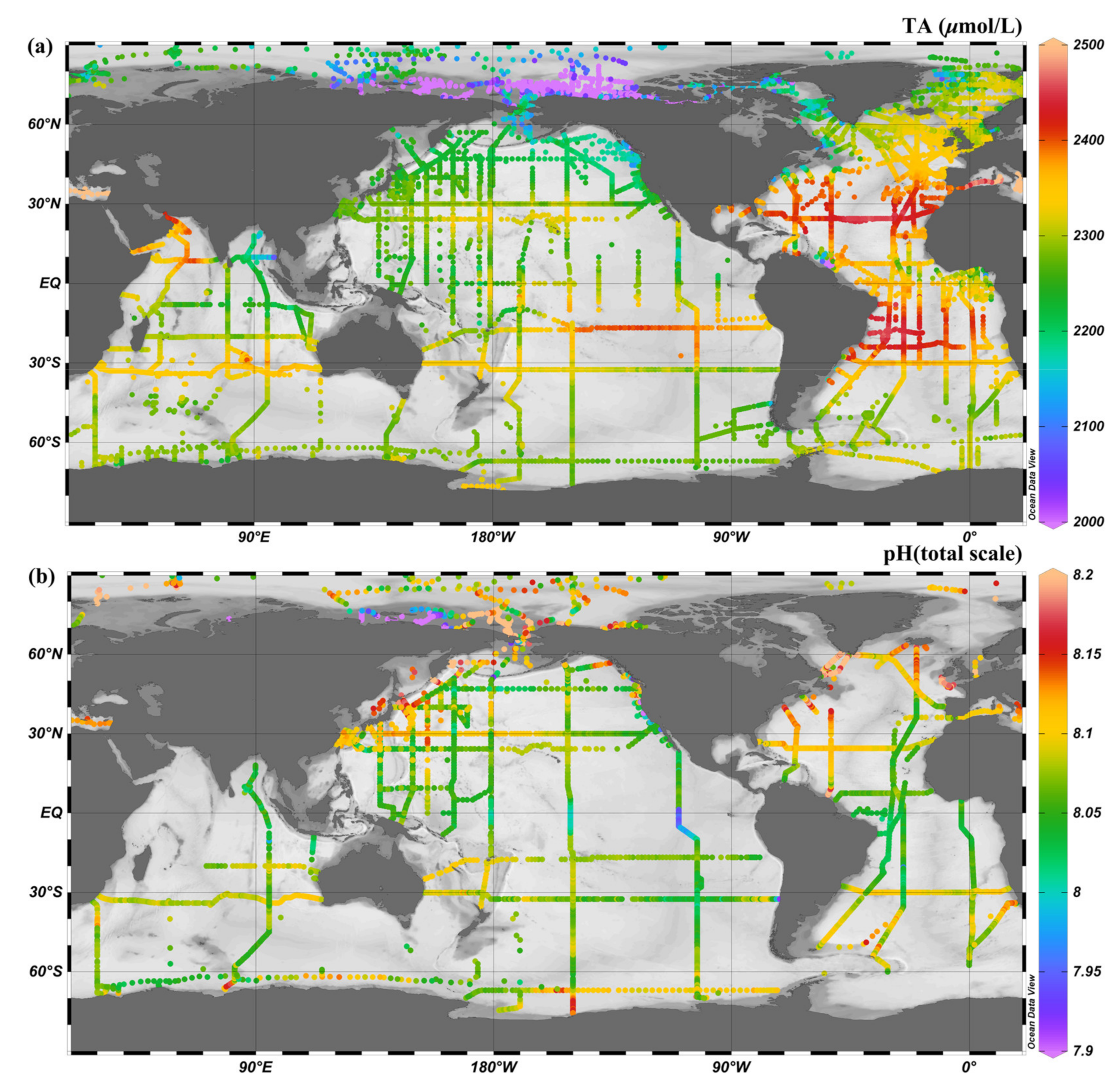
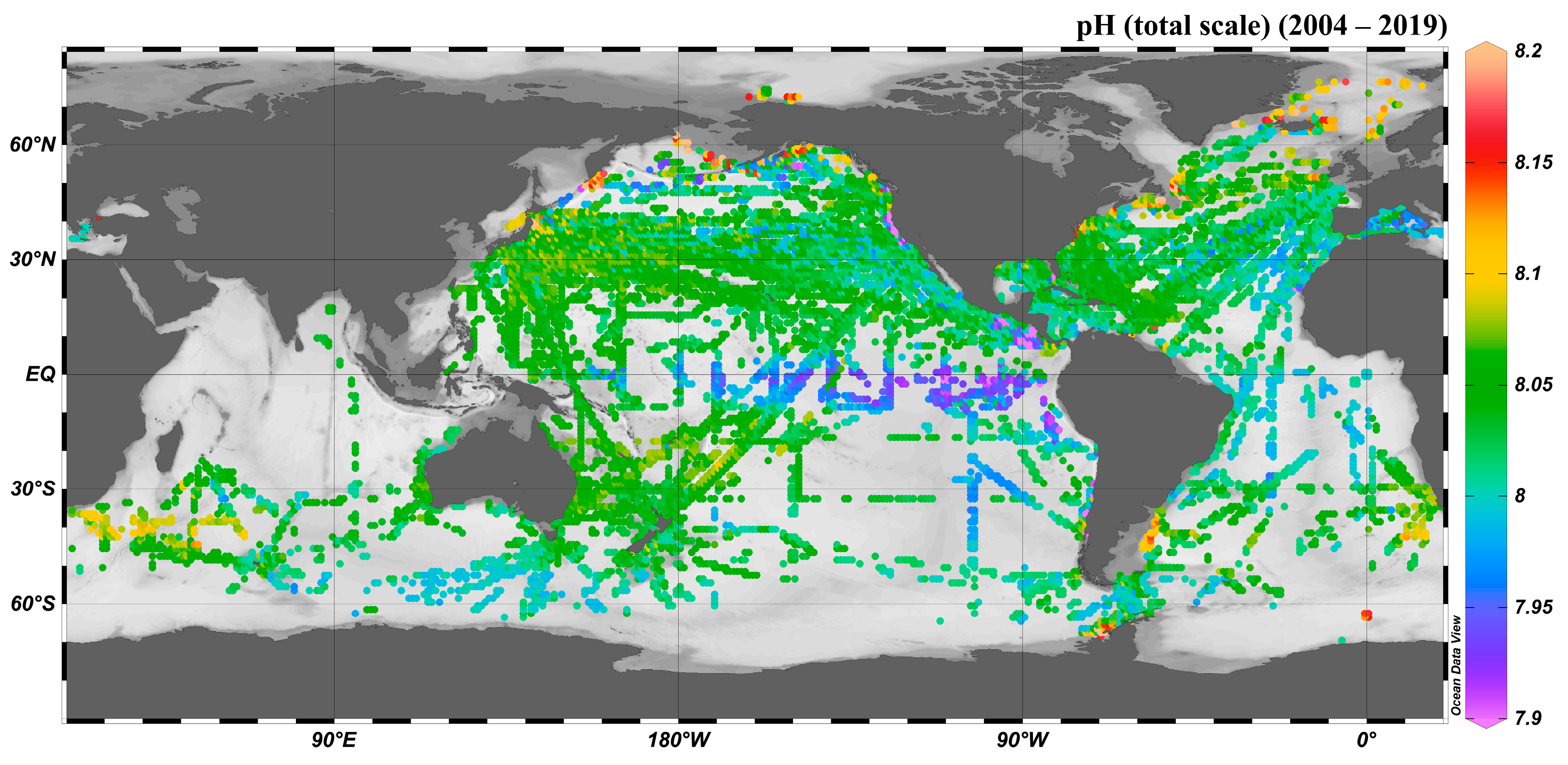
2.1. Field Data
2.2. Remote Sensing Data and Reanalysis Data
2.3. Calculation of the Seawater Carbonate System
2.4. Accuracy Evaluation Index
3. Algorithm Development and Validation
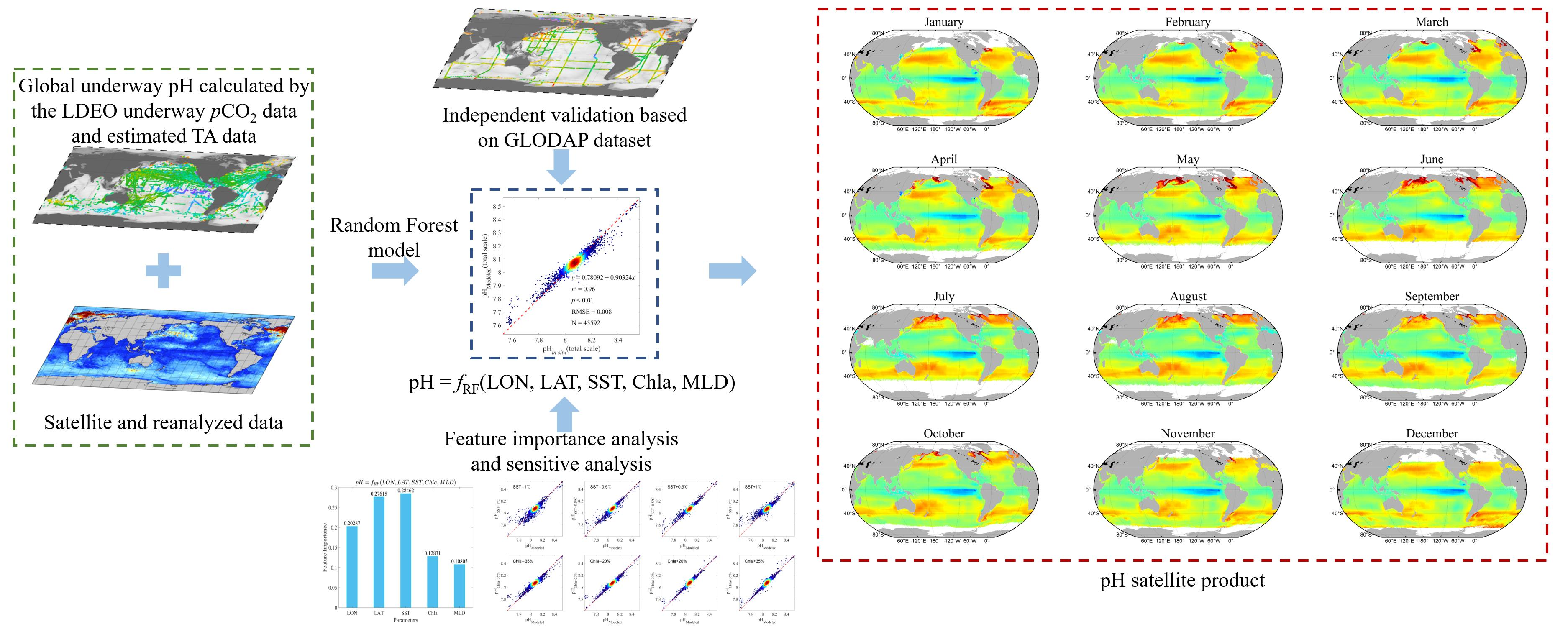
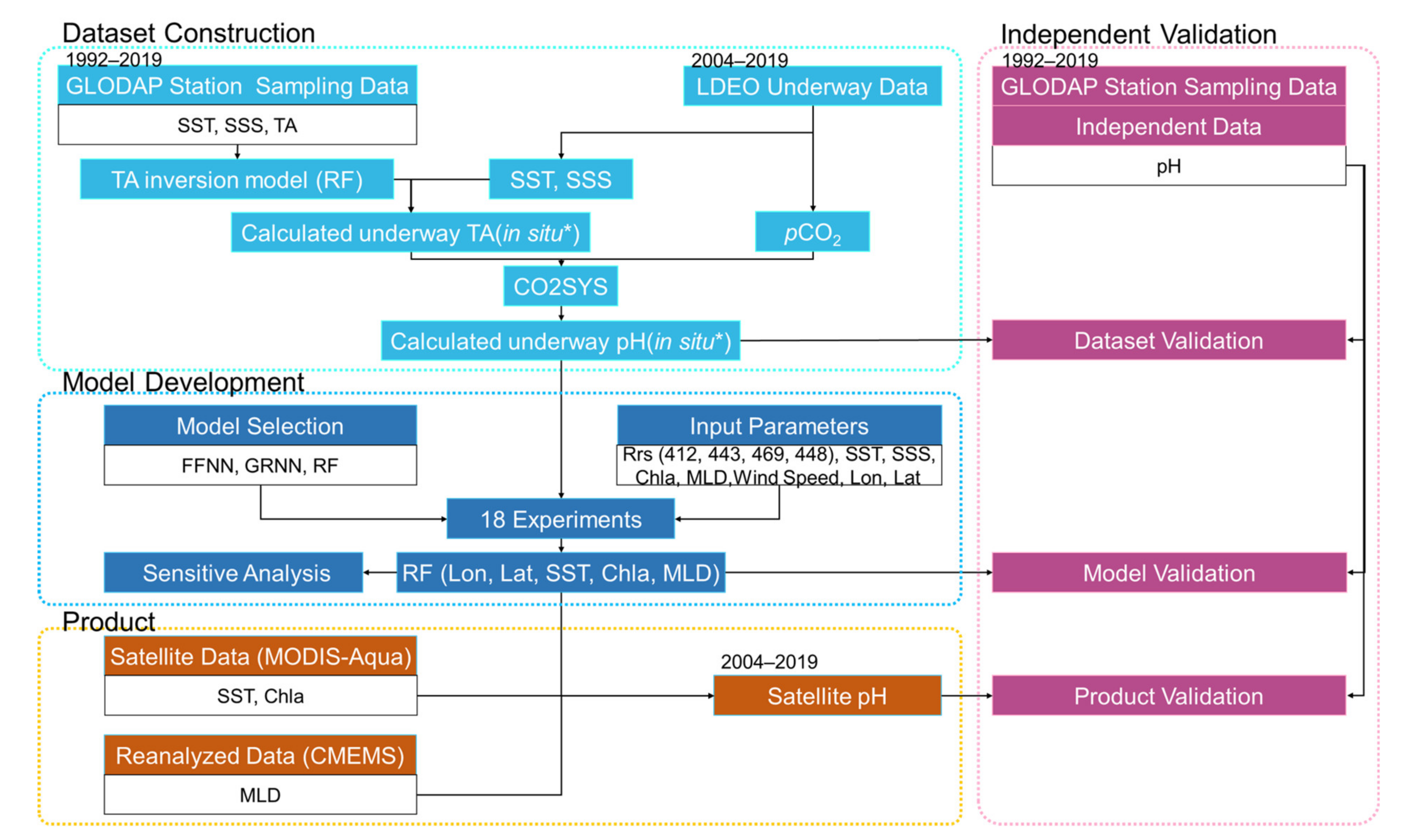
3.1. Overview of the pH Inversion Model Development
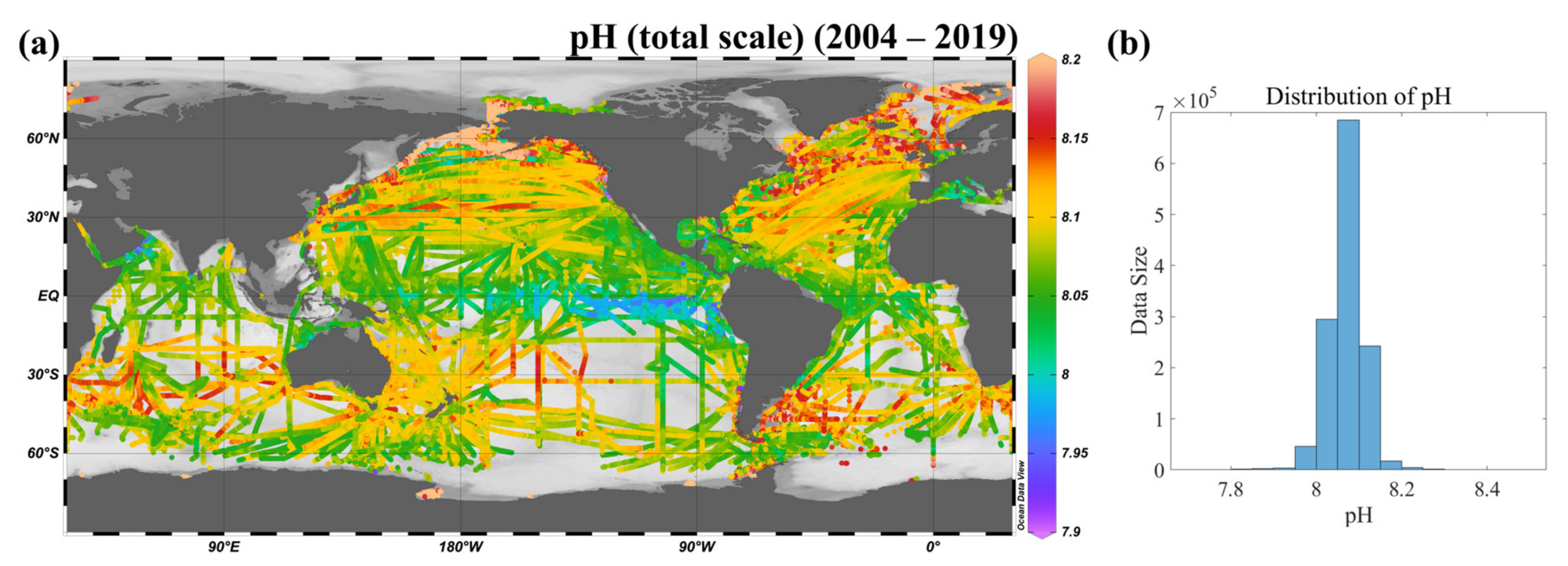
3.2. Construction of the near In Situ pH Dataset
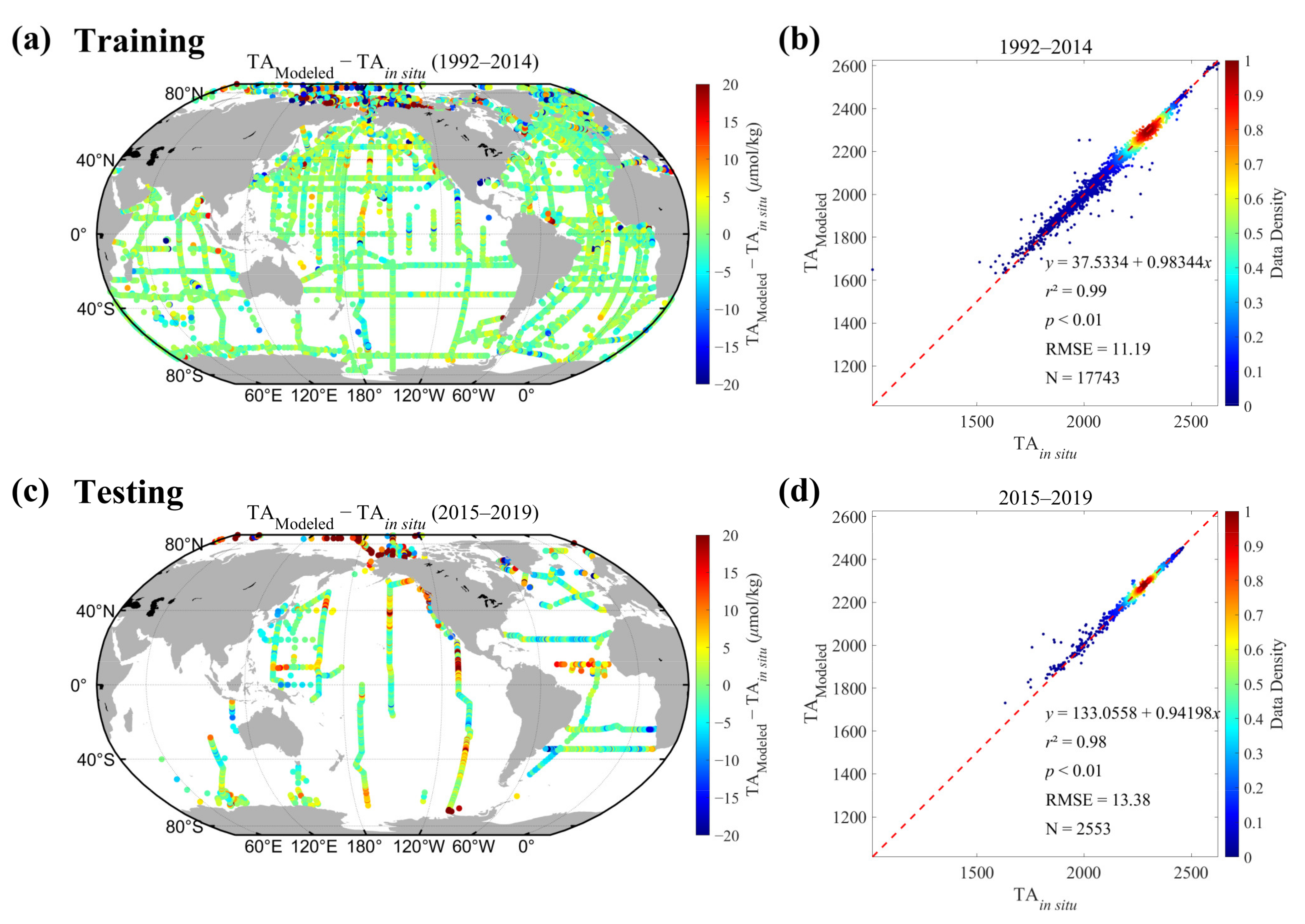
3.2.1. Construction of the Calculated near In Situ TA Dataset
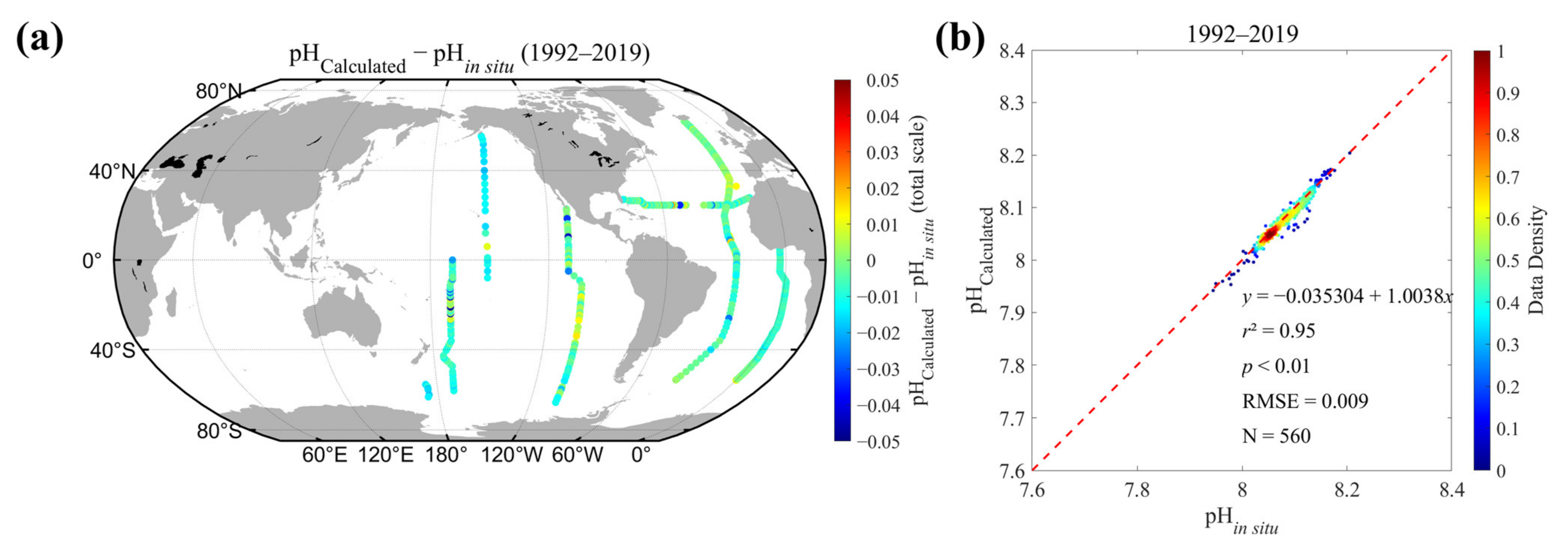
3.2.2. Construction and Validation of the Calculated near In Situ pH Dataset
3.3. Inversion Model of Satellite-Derived pH
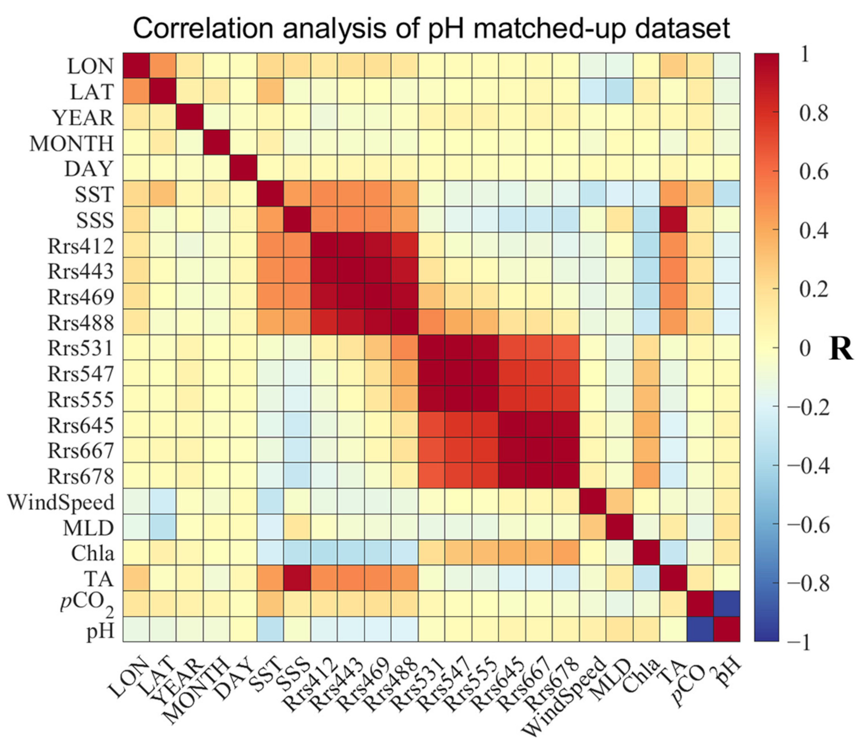
3.3.1. Matchup Dataset for pH Inversion
3.3.2. Machine Learning Models and Inputs
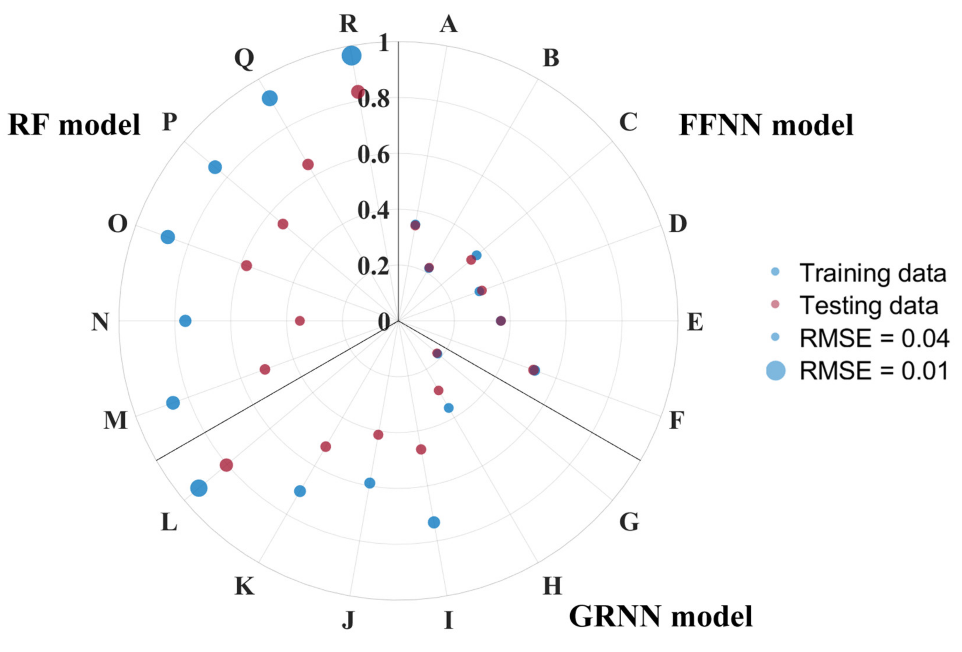
3.3.3. Model Experiments and Comparison
3.4. Validation of the Satellite-Derived pH Product
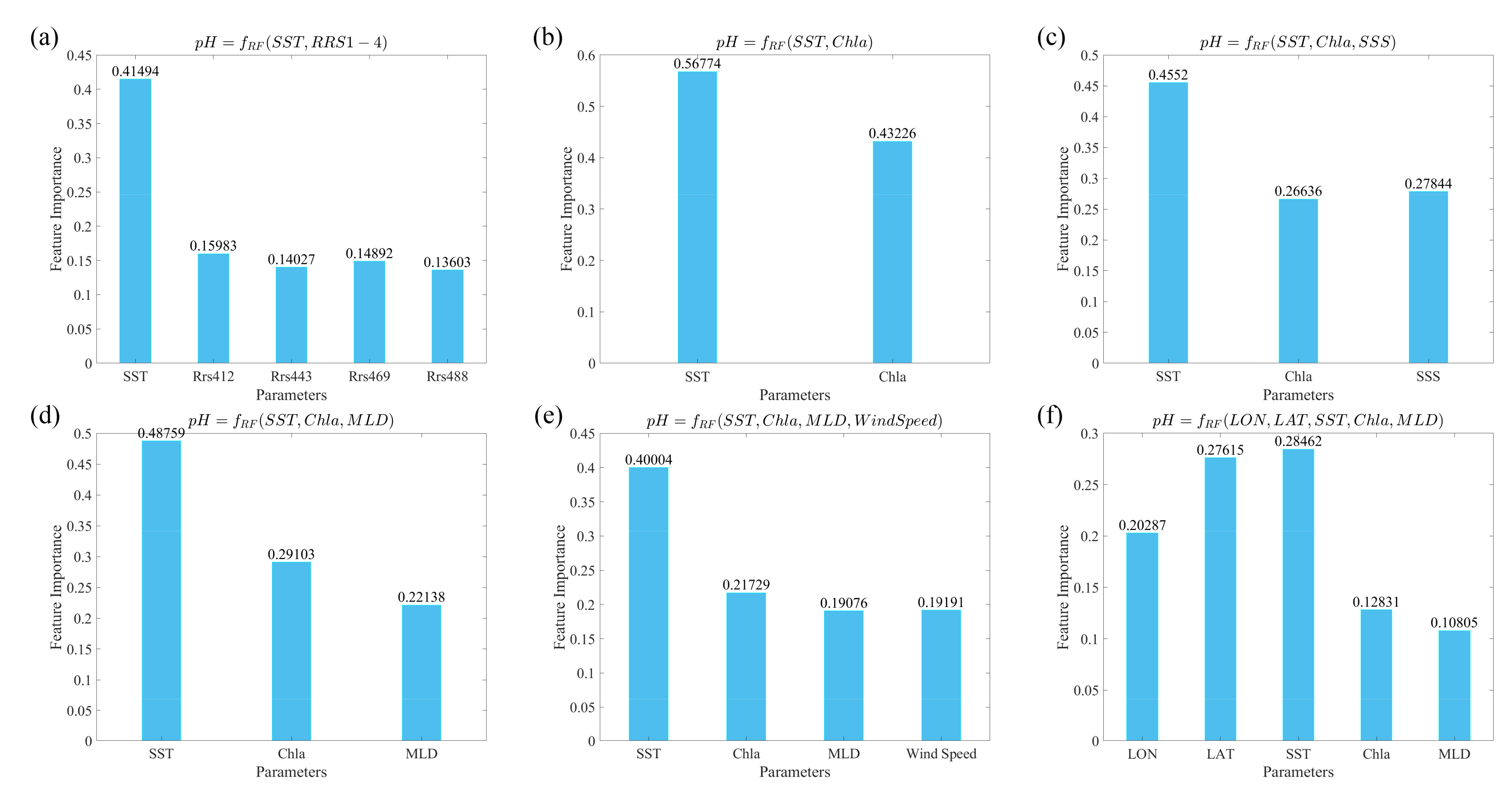
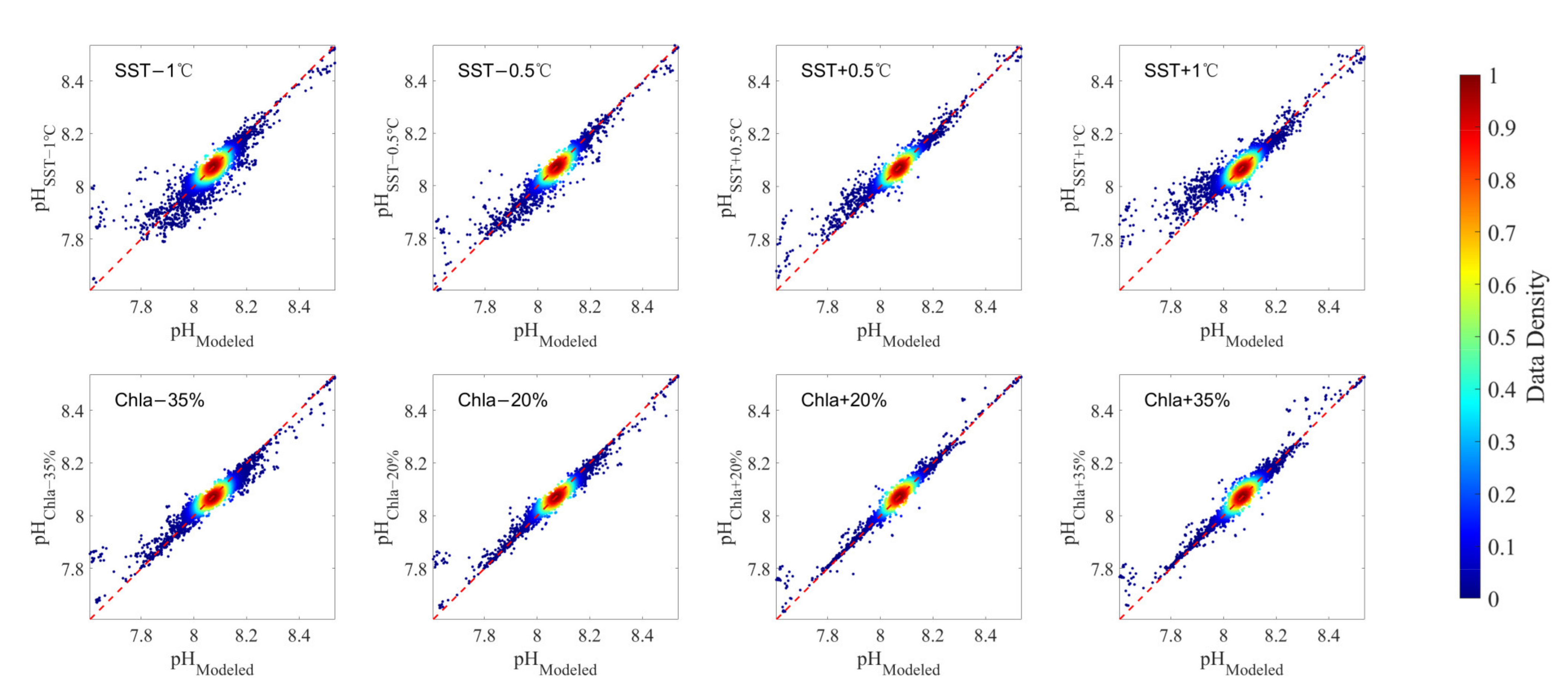
3.4.1. Sensitivity Analysis of the pH Model
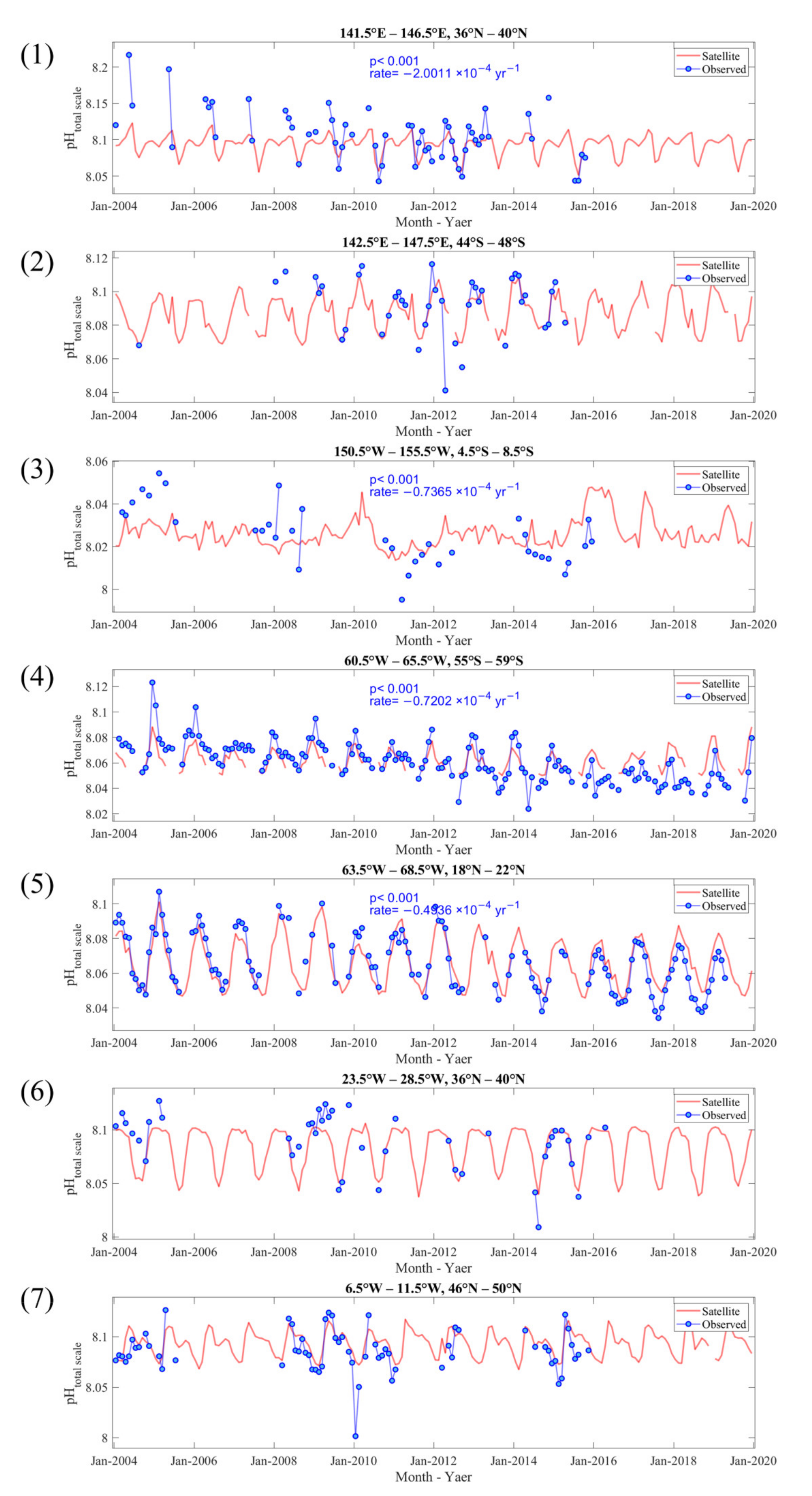
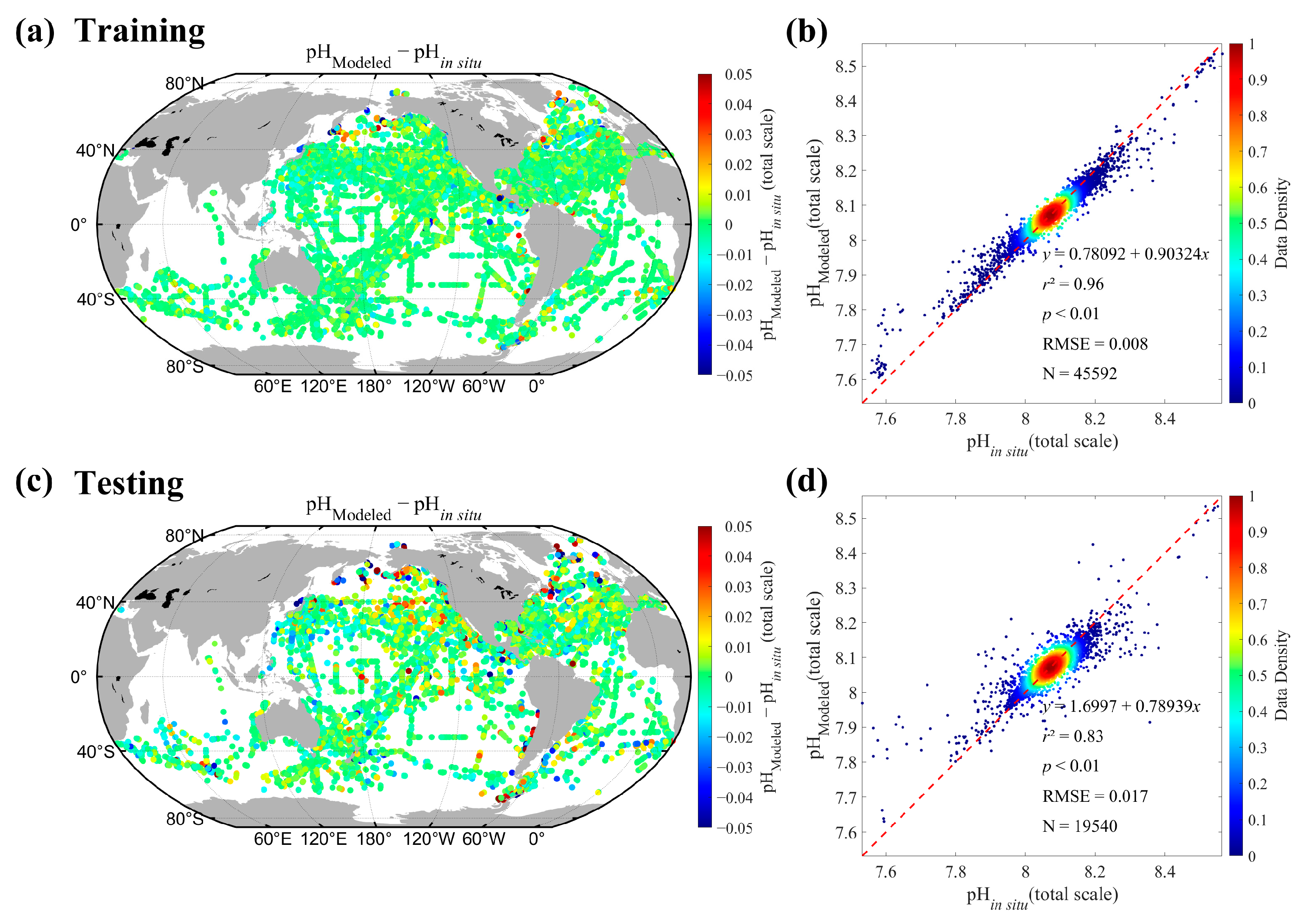
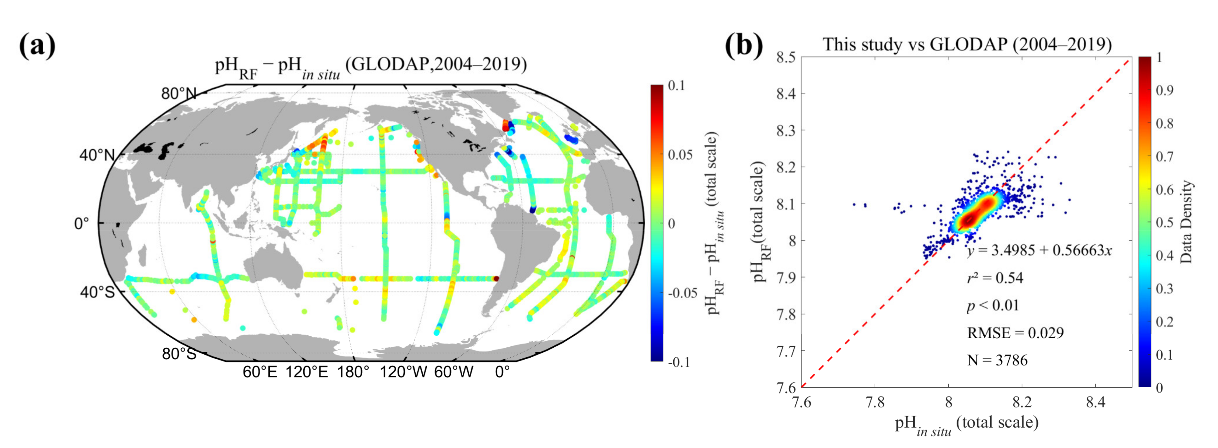
3.4.2. Validation of Satellite-Derived pH
4. Results and Discussion
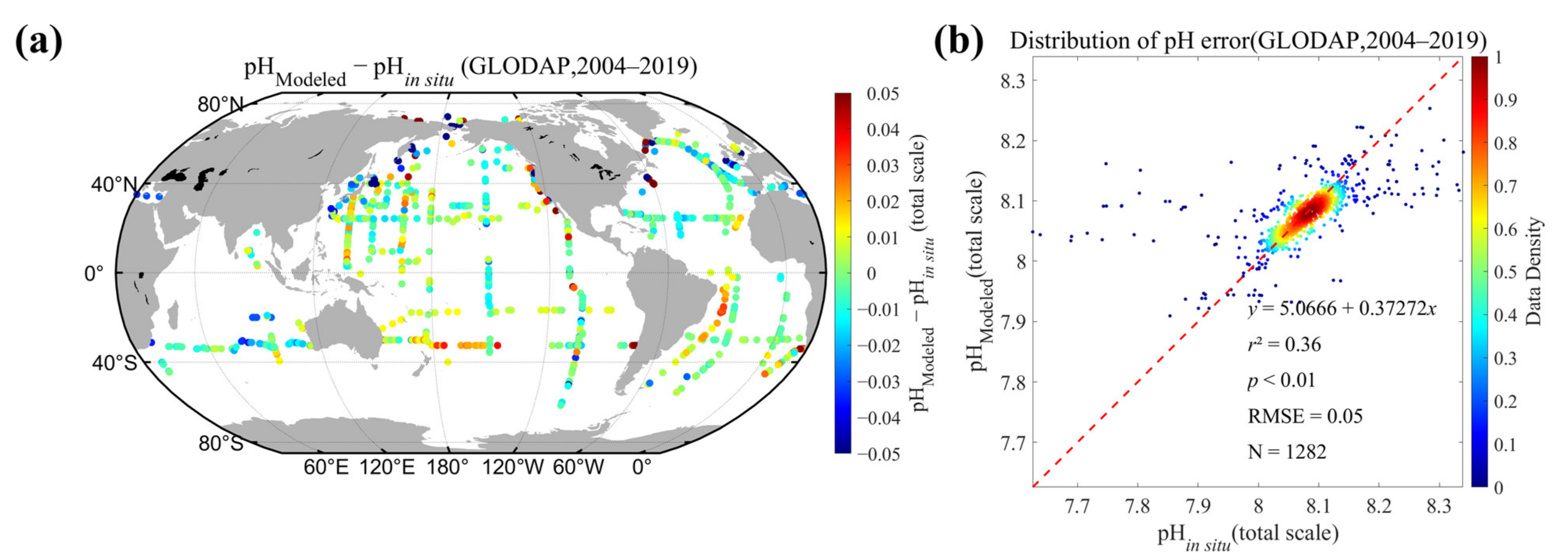
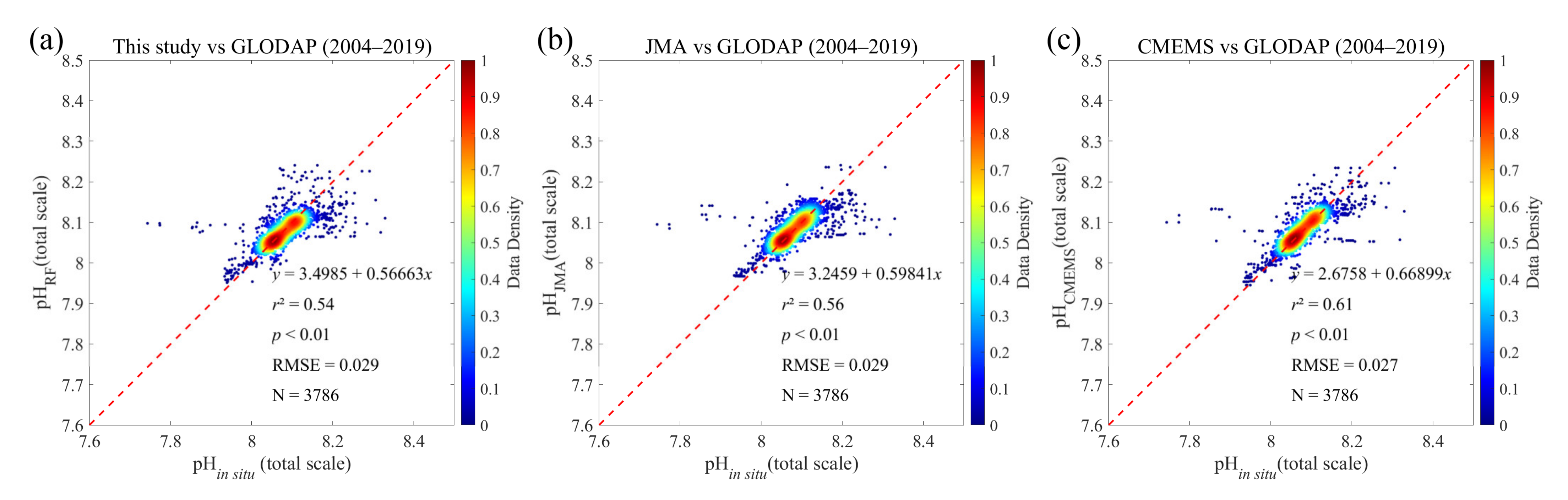
4.1. Comparison with Other pH Products
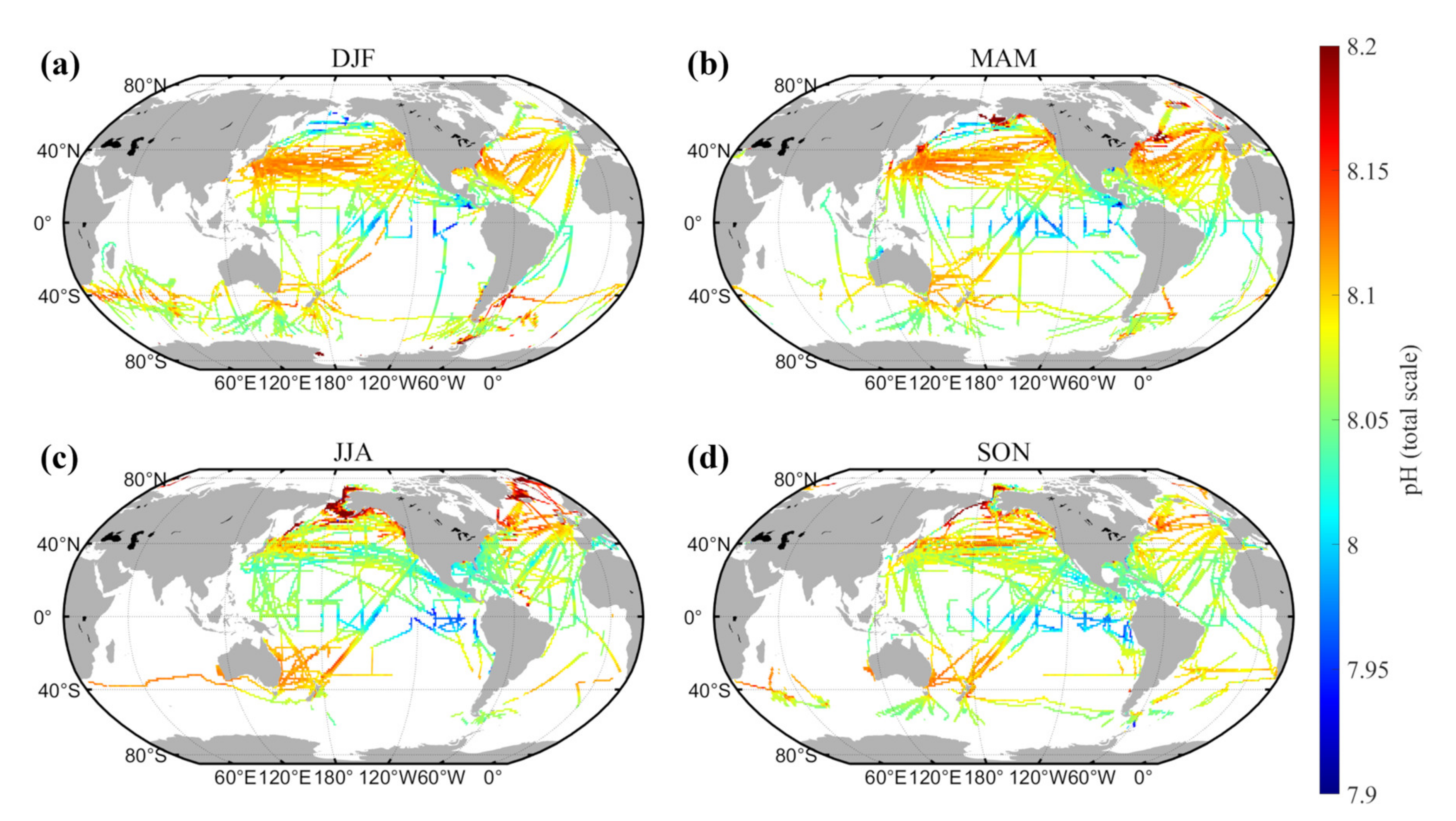
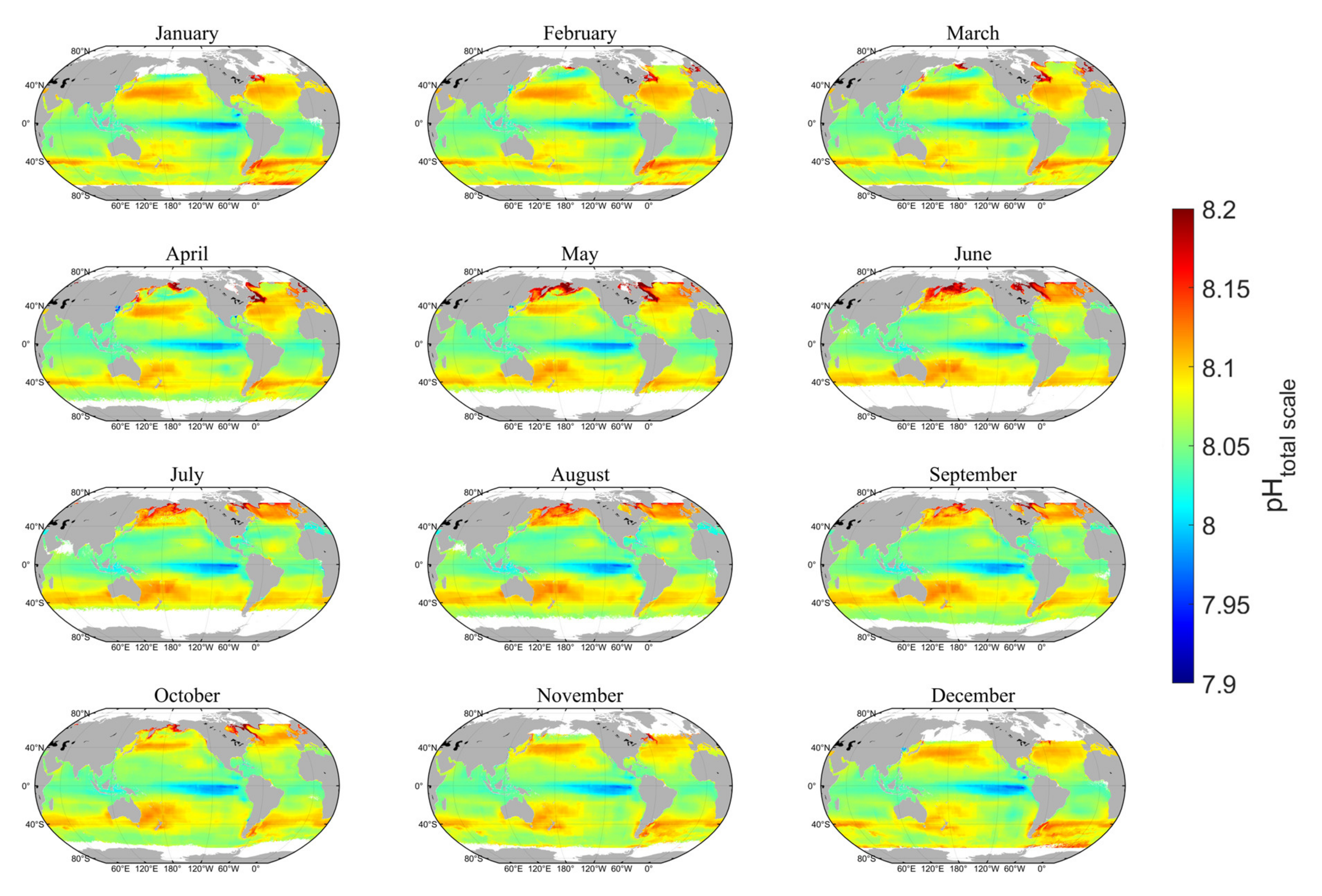
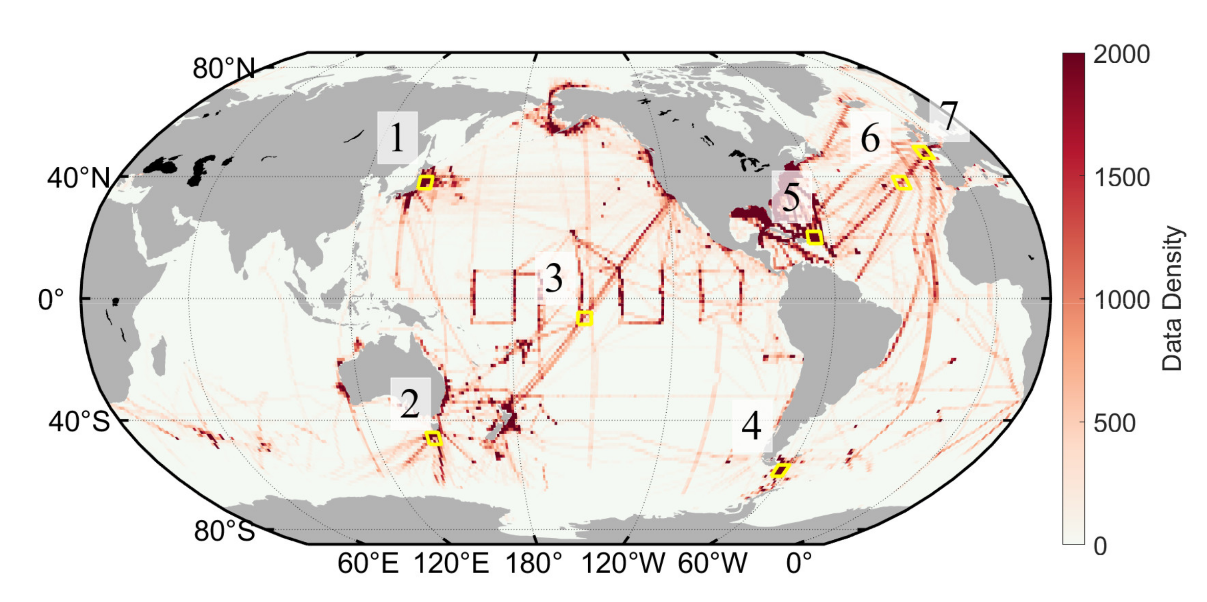
4.2. Spatial Distribution of Sea Surface pH
5. Conclusions
Author Contributions
Funding
Data Availability Statement
Acknowledgments
Conflicts of Interest
References
- Sabine, C.L.; Feely, R.A. The oceanic sink for carbon dioxide. In Greenhouse Gas Sinks; CABI: Wallingford, UK, 2007; p. 31. [Google Scholar]
- Sabine, C.L.; Feely, R.A.; Gruber, N.; Key, R.M.; Lee, K.; Bullister, J.L.; Wanninkhof, R.; Wong, C.; Wallace, D.W.; Tilbrook, B. The oceanic sink for anthropogenic CO2. Science 2004, 305, 367–371. [Google Scholar] [CrossRef] [PubMed] [Green Version]
- Friedlingstein, P.; O’sullivan, M.; Jones, M.W.; Andrew, R.M.; Hauck, J.; Olsen, A.; Peters, G.P.; Peters, W.; Pongratz, J.; Sitch, S. Global carbon budget 2020. Earth Syst. Sci. Data 2020, 12, 3269–3340. [Google Scholar] [CrossRef]
- Doney, S.C.; Fabry, V.J.; Feely, R.A.; Kleypas, J.A. Ocean acidification: The other CO2 problem. Annu. Rev. Mar. Sci. 2009, 1, 169–192. [Google Scholar] [CrossRef] [PubMed] [Green Version]
- Raven, J.; Caldeira, K.; Elderfield, H.; Hoegh-Guldberg, O.; Liss, P.; Riebesell, U.; Shepherd, J.; Turley, C.; Watson, A. Ocean Acidification Due to Increasing Atmospheric Carbon Dioxide; The Royal Society: London, UK, 2005. [Google Scholar]
- Marion, G.; Millero, F.J.; Camões, M.; Spitzer, P.; Feistel, R.; Chen, C.-T. pH of seawater. Mar. Chem. 2011, 126, 89–96. [Google Scholar] [CrossRef]
- Kim, J.; Kim, K.; Cho, J.; Kang, Y.Q.; Yoon, H.-J.; Lee, Y.-W. Satellite-based prediction of Arctic sea ice concentration using a deep neural network with multi-model ensemble. Remote Sens. 2019, 11, 19. [Google Scholar] [CrossRef] [Green Version]
- Riebesell, U.; Zondervan, I.; Rost, B.; Tortell, P.D.; Zeebe, R.E.; Morel, F.M. Reduced calcification of marine plankton in response to increased atmospheric CO2. Nature 2000, 407, 364–367. [Google Scholar] [CrossRef] [Green Version]
- Berge, T.; Daugbjerg, N.; Andersen, B.B.; Hansen, P.J. Effect of lowered pH on marine phytoplankton growth rates. Mar. Ecol. Prog. Ser. 2010, 416, 79–91. [Google Scholar] [CrossRef]
- Chen, C.Y.; Durbin, E.G. Effects of pH on the growth and carbon uptake of marine phytoplankton. Mar. Ecol.-Prog. Ser. 1994, 109, 83. [Google Scholar] [CrossRef]
- Hansen, P. Effect of high pH on the growth and survival of marine phytoplankton: Implications for species succession. Aquat. Microb. Ecol. 2002, 28, 279–288. [Google Scholar] [CrossRef]
- Hinga, K.R. Effects of pH on coastal marine phytoplankton. Mar. Ecol. Prog. Ser. 2002, 238, 281–300. [Google Scholar] [CrossRef]
- Jiang, L.-Q.; Carter, B.R.; Feely, R.A.; Lauvset, S.K.; Olsen, A. Surface ocean pH and buffer capacity: Past, present and future. Sci. Rep. 2019, 9, 1–11. [Google Scholar] [CrossRef]
- Pachauri, R.K.; Allen, M.R.; Barros, V.R.; Broome, J.; Cramer, W.; Christ, R.; Church, J.A.; Clarke, L.; Dahe, Q.; Dasgupta, P. Climate Change 2014: Synthesis Report. Contribution of Working Groups I, II and III to the Fifth Assessment Report of the Intergovernmental Panel on Climate Change; IPCC: Geneva, Switzerland, 2014. [Google Scholar]
- Caldeira, K.; Wickett, M.E. Anthropogenic carbon and ocean pH. Nature 2003, 425, 365. [Google Scholar] [CrossRef]
- Millero, F.J. The marine inorganic carbon cycle. Chem. Rev. 2007, 107, 308–341. [Google Scholar] [CrossRef]
- Sabia, R.; Fernández-Prieto, D.; Shutler, J.; Donlon, C.; Land, P.; Reul, N. Remote sensing of surface ocean PH exploiting sea surface salinity satellite observations. In Proceedings of the 2015 IEEE International Geoscience and Remote Sensing Symposium (IGARSS), Milan, Italy, 26–31 July 2015; pp. 106–109. [Google Scholar]
- Iida, Y.; Kojima, A.; Takatani, Y.; Nakano, T.; Sugimoto, H.; Midorikawa, T.; Ishii, M. Trends in pCO2 and sea–air CO2 flux over the global open oceans for the last two decades. J. Oceanogr. 2015, 71, 637–661. [Google Scholar] [CrossRef]
- Iida, Y.; Takatani, Y.; Kojima, A.; Ishii, M. Global trends of ocean CO2 sink and ocean acidification: An observation-based reconstruction of surface ocean inorganic carbon variables. J. Oceanogr. 2020, 77, 1–36. [Google Scholar] [CrossRef]
- Trang Chau, M.G.; Frédéric, C. Global Ocean Surface Carbon. 2021. Available online: https://resources.marine.copernicus.eu/product-detail/MULTIOBS_GLO_BIO_CARBON_SURFACE_REP_015_008/INFORMATION (accessed on 1 February 2022).
- Talling, J. The depletion of carbon dioxide from lake water by phytoplankton. J. Ecol. 1976, 64, 79–121. [Google Scholar] [CrossRef]
- Atkinson, P.M.; Tatnall, A.R. Introduction neural networks in remote sensing. Int. J. Remote Sens. 1997, 18, 699–709. [Google Scholar] [CrossRef]
- Keiner, L.E.; Yan, X.-H. A neural network model for estimating sea surface chlorophyll and sediments from thematic mapper imagery. Remote Sens. Environ. 1998, 66, 153–165. [Google Scholar] [CrossRef]
- Chen, S.; Hu, C. Estimating sea surface salinity in the northern Gulf of Mexico from satellite ocean color measurements. Remote Sens. Environ. 2017, 201, 115–132. [Google Scholar] [CrossRef]
- Breiman, L. Random forests. Mach. Learn. 2001, 45, 5–32. [Google Scholar] [CrossRef] [Green Version]
- Liu, J.; Weng, F.; Li, Z. Satellite-based PM2.5 estimation directly from reflectance at the top of the atmosphere using a machine learning algorithm. Atmos. Environ. 2019, 208, 113–122. [Google Scholar] [CrossRef]
- Chen, S.; Hu, C.; Barnes, B.B.; Wanninkhof, R.; Cai, W.-J.; Barbero, L.; Pierrot, D. A machine learning approach to estimate surface ocean pCO2 from satellite measurements. Remote Sens. Environ. 2019, 228, 203–226. [Google Scholar] [CrossRef]
- Takahashi, T.; Sutherland, S.; Kozyr, A. Global Ocean Surface Water Partial Pressure of CO2 Database: Measurements Performed During 1957–2019 (LDEO Database Version 2019) (NCEI Accession 0160492), Version 9.9; NOAA National Centers for Environmental Information: Silver Spring, MD, USA, 2020.
- Olsen, A.; Key, R.M.; Van Heuven, S.; Lauvset, S.K.; Velo, A.; Lin, X.; Schirnick, C.; Kozyr, A.; Tanhua, T.; Hoppema, M. The Global Ocean Data Analysis Project version 2 (GLODAPv2)–an internally consistent data product for the world ocean. Earth Syst. Sci. Data 2016, 8, 297–323. [Google Scholar] [CrossRef] [Green Version]
- Wentz, F.; Scott, J.; Hoffman, R.; Leidner, M.; Atlas, R.; Ardizzone, J. Remote Sensing Systems Cross-Calibrated Multi-Platform (CCMP) 6-Hourly Ocean Vector Wind Analysis Product on 0.25 deg grid, Version 2.0; Remote Sensing Systems: Santa Rosa, CA, USA, 2015. [Google Scholar]
- Drévillon, M.; Lellouche, J.M. Global Ocean Physics Reanalysis GLOBAL_MULTIYEAR_PHY_001_030. 2021. Available online: https://resources.marine.copernicus.eu/product-detail/GLOBAL_MULTIYEAR_PHY_001_030/INFORMATION (accessed on 1 February 2022).
- Lewis, E.; Wallace, D. Program Developed for CO2 System Calculations; Environmental System Science Data Infrastructure for a Virtual Ecosystem; Oak Ridge National Laboratory: Oak Ridge, TN, USA, 1998. [Google Scholar]
- Dickson, A.; Riley, J. The estimation of acid dissociation constants in seawater media from potentionmetric titrations with strong base. I. The ionic product of water—Kw. Mar. Chem. 1979, 7, 89–99. [Google Scholar] [CrossRef]
- Lueker, T.J.; Dickson, A.G.; Keeling, C.D. Ocean pCO2 calculated from dissolved inorganic carbon, alkalinity, and equations for K1 and K2: Validation based on laboratory measurements of CO2 in gas and seawater at equilibrium. Mar. Chem. 2000, 70, 105–119. [Google Scholar] [CrossRef]
- Brewer, P.G.; Bradshaw, A.; Williams, R. Measurements of total carbon dioxide and alkalinity in the North Atlantic Ocean in 1981. In The Changing Carbon Cycle; Springer: Berlin/Heidelberg, Germany, 1986; pp. 348–370. [Google Scholar]
- Millero, F.J.; Lee, K.; Roche, M. Distribution of alkalinity in the surface waters of the major oceans. Mar. Chem. 1998, 60, 111–130. [Google Scholar] [CrossRef]
- Jiang, Z.P.; Tyrrell, T.; Hydes, D.J.; Dai, M.; Hartman, S.E. Variability of alkalinity and the alkalinity-salinity relationship in the tropical and subtropical surface ocean. Glob. Biogeochem. Cycles 2014, 28, 729–742. [Google Scholar] [CrossRef] [Green Version]
- Lee, K.; Tong, L.T.; Millero, F.J.; Sabine, C.L.; Dickson, A.G.; Goyet, C.; Park, G.H.; Wanninkhof, R.; Feely, R.A.; Key, R.M. Global relationships of total alkalinity with salinity and temperature in surface waters of the world′s oceans. Geophys. Res. Lett. 2006, 33, 1–5. [Google Scholar] [CrossRef] [Green Version]
- Takatani, Y.; Enyo, K.; Iida, Y.; Kojima, A.; Nakano, T.; Sasano, D.; Kosugi, N.; Midorikawa, T.; Suzuki, T.; Ishii, M. Relationships between total alkalinity in surface water and sea surface dynamic height in the Pacific Ocean. J. Geophys. Res. Ocean. 2014, 119, 2806–2814. [Google Scholar] [CrossRef]
- Gentemann, C.L. Three way validation of MODIS and AMSR-E sea surface temperatures. J. Geophys. Res. Ocean. 2014, 119, 2583–2598. [Google Scholar] [CrossRef]
- Hu, C.; Feng, L.; Lee, Z. Uncertainties of SeaWiFS and MODIS remote sensing reflectance: Implications from clear water measurements. Remote Sens. Environ. 2013, 133, 168–182. [Google Scholar] [CrossRef]
- Moore, T.S.; Campbell, J.W.; Feng, H. Characterizing the uncertainties in spectral remote sensing reflectance for SeaWiFS and MODIS-Aqua based on global in situ matchup data sets. Remote Sens. Environ. 2015, 159, 14–27. [Google Scholar] [CrossRef]


| Parameters | Dataset | Data Type | Time | Spatial Resolution |
|---|---|---|---|---|
| pCO2, SST, SSS | Global Surface pCO2 (LDEO) Database | Field data | 2004–2019 | station sampling |
| pCO2, TA, pH, SSS, SST | GLODAP | Field data | 1992–2019 | station sampling |
| RRS, Chla | MODIS-Aqua | Satellite data | 2004–2019, daily | 4 km |
| Chla, SST | MODIS-Aqua | Satellite data | 2004–2019, monthly | 4 km |
| U-wind, V-wind | CCMP | Reanalyzed data | 2004–2019, daily | 0.25° × 0.25° |
| Mixed-layer depth | CMEMS GLOBAL_MULTIYEAR_PHY_001_030 | Reanalyzed data | 2004–2019, monthly | 4 km |
| Model | Input | n (Training) | Time | R2 | RMSE | n (Testing) | Time | R2 | RMSE | |
|---|---|---|---|---|---|---|---|---|---|---|
| 1 | FFNN | SST, SSS | 17,743 | 1992–2014 | 0.92 | 16.92 | 2553 | 2015–2019 | 0.97 | 12.08 |
| 2 | FFNN | LON, LAT, SST, SSS | 17,743 | 1992–2014 | 0.97 | 11.06 | 2553 | 2015–2019 | 0.98 | 9.35 |
| 3 | RF | SST, SSS | 17,743 | 1992–2014 | 0.98 | 9.39 | 2553 | 2015–2019 | 0.96 | 13.62 |
| 4 | RF | LON, LAT, SST, SSS | 17,743 | 1992–2014 | 0.99 | 11.19 | 2553 | 2015–2019 | 0.98 | 13.38 |
| pH | Lon | Lat | Year | Month | Day | SST | SSS | Rrs412 | Rrs443 | Rrs469 | Rrs488 |
| −0.13 | −0.12 | −0.08 | −0.08 | 0.01 | −0.32 | −0.05 | −0.18 | −0.19 | −0.20 | −0.20 | |
| Rrs531 | Rrs547 | Rrs555 | Rrs645 | Rrs667 | Rrs678 | Wind Speed | MLD | Chla | TA | pCO2 | |
| −0.02 | 0.02 | 0.03 | 0.06 | 0.04 | 0.06 | 0.08 | 0.15 | 0.13 | −0.04 | −0.95 |
| Model | Order | Parameters | Training (n = 45,592) | Testing (n = 19,540) | ||
|---|---|---|---|---|---|---|
| R2 | RMSE | R2 | RMSE | |||
| FFNN | A | SST, RRS1-4 | 0.35 | 0.036 | 0.35 | 0.035 |
| B | SST, CHL | 0.22 | 0.039 | 0.22 | 0.039 | |
| C | SST, CHL, SSS | 0.37 | 0.035 | 0.34 | 0.036 | |
| D | SST, CHL, MLD | 0.31 | 0.037 | 0.32 | 0.036 | |
| E | SST, CHL, MLD, WS | 0.37 | 0.035 | 0.37 | 0.035 | |
| F | LON, LAT, SST, CHL, MLD | 0.52 | 0.031 | 0.51 | 0.030 | |
| GRNN | G | SST, RRS1-4 | 0.18 | 0.040 | 0.18 | 0.040 |
| H | SST, CHL | 0.36 | 0.035 | 0.29 | 0.037 | |
| I | SST, CHL, SSS | 0.73 | 0.023 | 0.47 | 0.032 | |
| J | SST, CHL, MLD | 0.59 | 0.028 | 0.41 | 0.034 | |
| K | SST, CHL, MLD, WS | 0.70 | 0.024 | 0.52 | 0.030 | |
| L | LON, LAT, SST, CHL, MLD | 0.93 | 0.012 | 0.80 | 0.019 | |
| RF | M | SST, RRS1-4 | 0.86 | 0.018 | 0.51 | 0.031 |
| N | SST, CHL | 0.76 | 0.023 | 0.35 | 0.035 | |
| O | SST, CHL, SSS | 0.88 | 0.017 | 0.58 | 0.028 | |
| P | SST, CHL, MLD | 0.86 | 0.018 | 0.54 | 0.030 | |
| Q | SST, CHL, MLD, WS | 0.92 | 0.014 | 0.65 | 0.026 | |
| R | LON, LAT, SST, CHL, MLD | 0.96 | 0.009 | 0.83 | 0.018 | |
| Cases | R2 | RMSE | MB | Cases | R2 | RMSE | MB |
|---|---|---|---|---|---|---|---|
| SST − 1 °C | 0.94 | 0.013 | 0.0031 | Chla − 35% | 0.97 | 0.011 | −0.0004 |
| SST − 0.5 °C | 0.98 | 0.008 | 0.0016 | Chla − 20% | 0.98 | 0.007 | −0.0003 |
| SST + 0.5 °C | 0.98 | 0.008 | −0.0012 | Chla + 20% | 0.99 | 0.006 | 0.0008 |
| SST + 1 °C | 0.95 | 0.013 | −0.0025 | Chla + 35% | 0.98 | 0.008 | 0.0013 |
| Sea Area | Longitude | Latitude | |
|---|---|---|---|
| 1 | Northwest Pacific Ocean | 141.5–146.5°E | 36–40°N |
| 2 | South of Australia | 142.5–147.5°E | 44–48°S |
| 3 | Equatorial Pacific Ocean | 150.5–155.5°W | 4.5–8.5°S |
| 4 | South of South America | 60.5–65.5°W | 55–59°S |
| 5 | North of Puerto Rico | 63.5–68.5°W | 18–22°N |
| 6 | Mid North Atlantic Ocean | 23.5–28.5°W | 36–40°N |
| 7 | Northeast Atlantic Ocean | 6.5–11.5°W | 46–50°N |
Publisher’s Note: MDPI stays neutral with regard to jurisdictional claims in published maps and institutional affiliations. |
© 2022 by the authors. Licensee MDPI, Basel, Switzerland. This article is an open access article distributed under the terms and conditions of the Creative Commons Attribution (CC BY) license (https://creativecommons.org/licenses/by/4.0/).
Share and Cite
Jiang, Z.; Song, Z.; Bai, Y.; He, X.; Yu, S.; Zhang, S.; Gong, F. Remote Sensing of Global Sea Surface pH Based on Massive Underway Data and Machine Learning. Remote Sens. 2022, 14, 2366. https://doi.org/10.3390/rs14102366
Jiang Z, Song Z, Bai Y, He X, Yu S, Zhang S, Gong F. Remote Sensing of Global Sea Surface pH Based on Massive Underway Data and Machine Learning. Remote Sensing. 2022; 14(10):2366. https://doi.org/10.3390/rs14102366
Chicago/Turabian StyleJiang, Zhiting, Zigeng Song, Yan Bai, Xianqiang He, Shujie Yu, Siqi Zhang, and Fang Gong. 2022. "Remote Sensing of Global Sea Surface pH Based on Massive Underway Data and Machine Learning" Remote Sensing 14, no. 10: 2366. https://doi.org/10.3390/rs14102366
APA StyleJiang, Z., Song, Z., Bai, Y., He, X., Yu, S., Zhang, S., & Gong, F. (2022). Remote Sensing of Global Sea Surface pH Based on Massive Underway Data and Machine Learning. Remote Sensing, 14(10), 2366. https://doi.org/10.3390/rs14102366