A New Coupling Method for PM_2.5 Concentration Estimation by the Satellite-Based Semiempirical Model and Numerical Model

Abstract

Aerosol optical and chemical properties play a major role in the retrieval of PM_2.5 concentrations based on aerosol optical depth (AOD) data from satellites in the conventional semiempirical model (SEM). However, limited observation information hinders the high-resolution estimation of PM_2.5. Therefore, a new method for evaluating near-surface PM_2.5 at high spatial resolution is developed by coupling the SEM and the chemical transport model (CTM)-based numerical (CSEN) model. The numerical model can provide large-scale information for aerosol properties with high spatial resolution at a large scale based on emissions and meteorology, though it can still be biased in simulating absolute PM_2.5 concentrations. Therefore, the two crucial aerosol characteristic parameters, including the coefficient integrated humidity effect (γ′) and the comprehensive reference value of aerosol properties (K) in SEM, have been redefined using the WRF-Chem numerical model. Improved model performance was observed for these results compared with the original SEM results. The monthly averaged correlation coefficients (R) by CSEN were 0.92, 0.82, 0.84, and 0.83 in January, April, July, and October, respectively, whereas those of the SEM were 0.80, 0.77, 0.72, and 0.72, respectively. All the statistical metrics of the model validation showed significant improvements in all seasons. The reduced biases of estimated PM_2.5 by CSEN indicated the effect of hygroscopic growth and aerosol properties affected by the meteorology on the relationship between AOD and estimated PM_2.5 concentrations, especially in winter and summer. The better performance of the CSEN model provides insight for air quality monitoring at different scales, which supplies important information for air pollution control policies and health impact analysis.

1. Introduction

Fine particulate matter (PM_2.5) consists of a complicated mixture of chemical compounds, mainly including organic carbon (OC), elemental carbon (EC), nitrate, sulfate, ammonium salt, sodium salt (Na +), and water [1,2]. Although Chinese government authorities have implemented strict atmospheric pollution control measures in recent years, significant pollution episodes and haze events still occur frequently in several regions in China. In most cases, the concentration of PM_2.5 in various areas can also reach values higher than the WHO standard (5 μg/m³). PM_2.5 is related to various environmental and climate effects and adverse human health impacts [3,4,5,6,7]. Although nationwide ground-based PM_2.5 monitoring networks have already been implemented around China, generating larger-scale high-resolution PM_2.5 estimation is still challenging, hindering the understanding of the PM_2.5 variation at diverse spatial scales. Therefore, to further understand the spatiotemporal distribution, transport paths, and formation mechanisms of PM_2.5, it is imperative to develop a ground-based higher spatial resolution PM_2.5 concentration estimation method at a large scale [8].

Satellite remote sensing observations cannot directly provide PM_2.5 concentrations even though they can obtain high spatial resolution aerosol extinction information at a large scale [9,10,11,12,13]. Previous studies attempt to retrieve PM_2.5 from aerosol optical depth (AOD) data and supplementary data by different AOD-PM_2.5 models. Most of these current models are still based on statistical methods or machine learning methods [12,13,14,15,16,17,18]. Although these models can quickly convert AOD into PM_2.5 via meteorological and land-use parameters, the generalization of these models to different areas is still limited due to the lack of physical interpretability and predictability [12].

The semiempirical model (SEM, i.e., a physical model) does not rely on geographical data but instead relies on the physical mechanism of the relationship between AOD and PM_2.5 [19] In SEMs, aerosol characteristics, such as hygroscopic growth, particle mass extinction efficiency, and size distribution, affect the relationship between the AOD and PM_2.5 concentration. This relationship can be obtained based upon long-term observations, including AOD, PM_2.5, and meteorological data. The SEM combines meteorological data with the PM_2.5 measurement to estimate indicators describing the integrated humidity effect, which is mainly affected by the aerosol composition and size distribution [20,21,22,23,24,25,26,27]. The updated SEM proposed by Li et al. (2015) showed that the accuracy of PM_2.5 estimation was improved markedly by incorporating the aerosol characteristics into the physical model [19]. Because of its robustness, relatively low computational cost, and the same degree of accuracy compared with other empirical models, the updated technique is suitable for operational use. However, since the SEM model relies heavily on ground-based observations at discrete locations, it is difficult to obtain high resolution temporal and spatial variability in aerosol properties [12].

Chemical transport models (CTMs) have already been applied to simulate PM_2.5 in many areas globally [28]. CTMs can supply extensive gridded simulated data of meteorology and physical and chemical properties of particulate matter. CTM-based approaches consider both meteorology (i.e., the height of the boundary layer and relative humidity (RH)) and aerosol physical properties (i.e., aerosol size distribution and aerosol types) [1,28,29]. These data are further combined into a simple empirical model to acquire the PM_2.5 concentrations from AOD. However, CTM-based approaches are mainly used in global PM_2.5 estimation. They are rarely used in non-global-scale research, mainly because the high operational cost and uncertainties of long-term CTM outputs [12]. However, with detailed emission information at high spatial resolution driven by realistic meteorology, the overall aerosol characteristic pattern simulated could be relatively reliable [30,31,32,33,34,35,36].

Given the respective advantages of SEMs and CTMs, we propose a new coupled model taking advantage of the improved physical mechanism between the AOD and PM_2.5 in SEM and the numerical models in providing high spatial resolution of aerosol properties to optimize the aerosol parameters required for the PM_2.5 estimation by the SEM. The rest of this paper is described below. The Materials and Methods section introduces the data used, including the observational meteorological and air quality dataset, satellite data, and Weather Research and Forecasting with Chemistry (WRF-Chem model) data. The difference between the CSEN method and the SEM is also discussed. The estimated aerosol parameters by conventional SEM and CSEN are analyzed in the Results section. In addition, satellite-derived PM_2.5 results based on the SEM and CSEN are compared with the ground-based observations. Furthermore, the seasonal variation in spatial distribution and major cluster distribution are also presented. In the Discussion and Conclusion section, we compare satellite-derived PM_2.5 results based on the SEM and CSEN concerning the overall accuracy.

2. Materials and Methods

2.1. MODIS AOD Data

The MODIS sensors aboard NASA’s satellites named Terra and Aqua have a return visit period of 1–2 days, offering daily near-global observations of the Earth. Terra and Aqua pass the equator at local times of approximately 10:30 am and 1:30 pm, respectively, therefore providing sustained daily monitoring of aerosols around the Earth. The 1-km-resolution MODIS AOD retrieved by the aerosol retrieval algorithm proposed by Lin et al. (2015) is used in this study [25]. The retrieved AOD is validated by AERONET version 3.0 level 1.5 at seven observed stations (

Table A1. Longitudes and latitudes of the AERONET sites used in this study.

Site	Latitude	Longitude
Beijing	39.977°N	116.381°E
Beijing CAMS	39.933°N	116.317°E
Beijing_PKU	39.992°N	116.31°E
Beijing RADI	40.005°N	116.379°E
Xianghe	39.754°N	116.962°E
XuZhou_CUMT	34.217°N	117.142°E
Hong Kong Sheung	22.483°N	114.117°E

) (see Appendix A). The positions of the seven observed stations are shown in Figure A1 (see Appendix A). Here, the observation times of MODIS and AERONET are consistent. Thus, we proposed a collocation method of spatiotemporal consistency. The space configuration standard is a 10 km radius at each AERONET site for a MODIS AOD value spatial average. AERONET AODs are interpolated to 0.55 μm to match the MODIS product wavelength and then temporally averaged within a window of ± 30 min of the satellite transit time. Figure A2 (see Appendix A) illustrates the relationship of paired AOD at all the AERONET sites over the study region (100°E to 125°E, 18°N to 45°N) in 2019. The scatter plots show a good agreement between MODIS AOD and AERONET AOD, with a correlation coefficient of 0.88 and mean bias (MB) of 0.19 (N = 278).

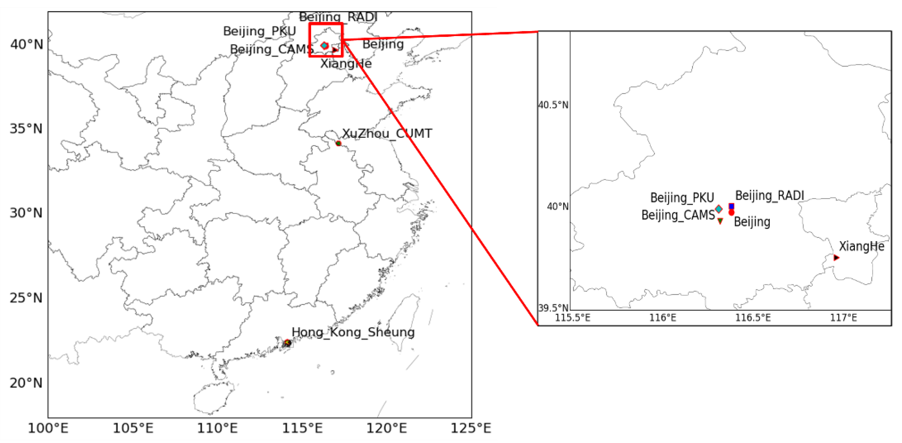
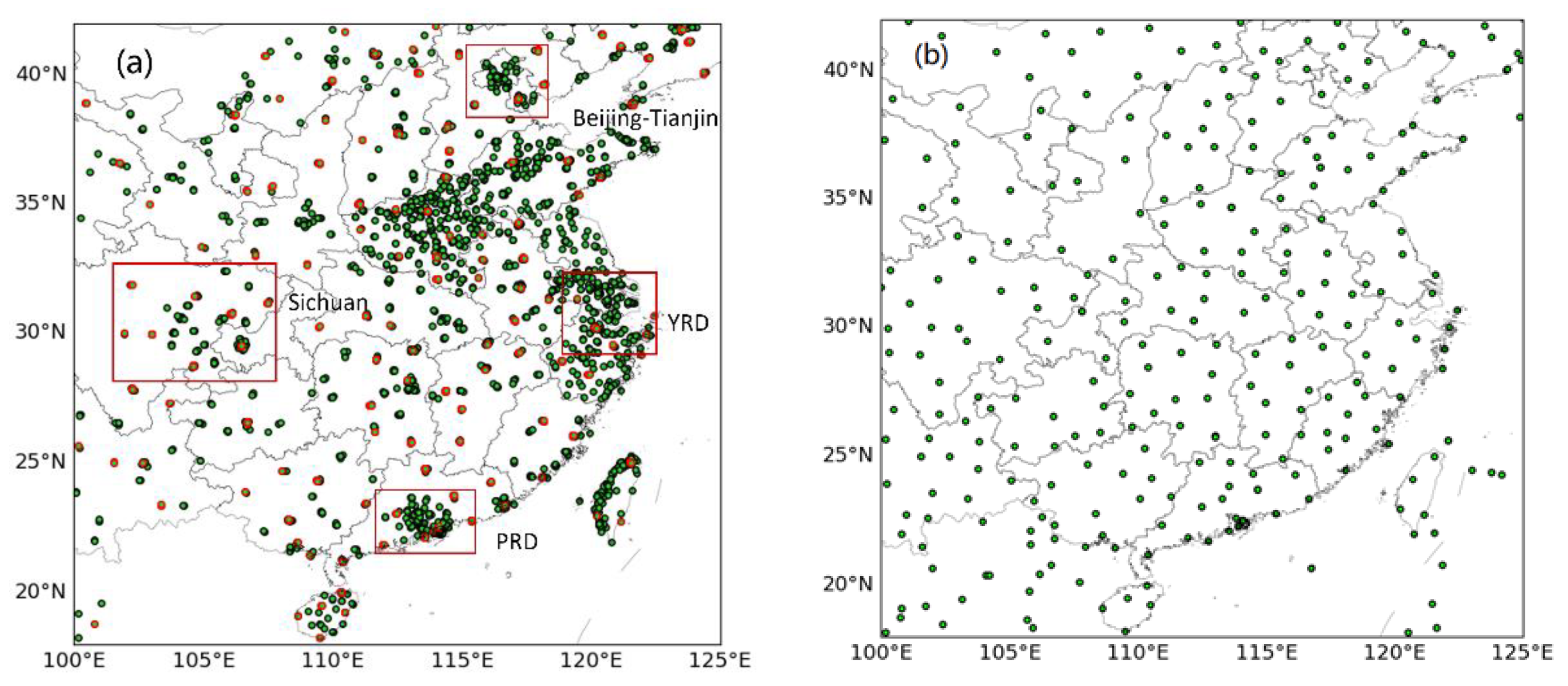
2.2. Ground Monitoring Data

The hourly concentrations of PM_2.5 data, measured at Air Quality Monitoring Stations (AQMS), in mainland China, Hong Kong, and Taiwan were obtained from the Ministry of Environmental Protection of China (MEPA), the Hong Kong Environmental Protection Department, and the Taiwan Environmental Protection Administration, respectively. Hourly measurements, including the RH and visibility (L), were obtained from the national China Meteorological Administration (CMA) surface observation network, which includes 297 global telecommunication system (GTS) stations in the study region. The locations of the PM_2.5 AQMS and GTS stations are presented in Figure 1a,b.

The hourly PM_2.5 concentration and hourly meteorological parameters were measured at different stations over the study region. Since PM_2.5 mass concentration and meteorological parameter values generally change smoothly at the regional scale, PM_2.5 monitoring sites and GTS stations in a window of 5 km distance can be matched. For this study, the meteorological data at 11:00 am and 2:00 pm were extracted to match the passage times of Terra and Aqua, respectively. We found that 271 GTS observation sites could be matched with 301 PM_2.5 sites. As a result, each site pair (2 × 365 days) has a maximum of 730 valid data points. The meteorological and PM_2.5 data obtained from the 301 matching stations were administered as a calibration database applied to build the AOD–PM_2.5 model. The ground-measured PM_2.5 data at 11:00 am and 2:00 pm were used to validate the satellite-derived hourly PM_2.5 data. The data from the remaining 1695 AQMS monitoring sites were used as a validation database to evaluate the accuracy of the estimated concentrations of PM_2.5 mass. Various monitoring stations are superimposed on a map (Figure 1a). This map shows that the PM_2.5 monitoring sites are concentrated in the main urban areas, whereas the coverage rate in rural areas is much lower.

2.3. The SEM

In the SEM, the aerosol hygroscopic growth effect, and the mass extinction efficiency (MEE) are the main elements linking the ground-level PM_2.5 mass concentration and satellite-retrieved AOD [19,25,26,27]. To make the paper self-contained, we briefly summarize the key equations of the SEM model in this section. The details of the derivation process can be found in Lin et al. (2015) and Li et al. (2015) [19,25].

The physical relationship between the PM_2.5 concentration and aerosol extinction coefficient at ground level driven by the hygroscopic growth can be described using Equation (1):

$$P{M}_{2.5}=\frac{ext}{\frac{{\alpha }_{ext,10}^{\prime }}{F}\times {\left(\frac{1-R{H}_i}{1-R{H}_0}\right)}^{-{\gamma }^{\prime }}}=\frac{ext}{K\times {\left(\frac{1-R{H}_i}{1-R{H}_0}\right)}^{-{\gamma }^{\prime }}}$$

(1)

where ext is the ground-level aerosol extinction coefficient, which is calculated based on the observed visibility. ${\alpha }_{ext,10}^{\prime }$ represents the reference mass extinction efficiency (MEE) of mixed aerosols at 0.55 μm under the condition of RH = RH₀. RH₀ is the reference RH value, which generally is set at 40% to represent dry conditions. F represents the fine mode fraction (FMF), which is equal to the ratio of PM_2.5 and PM₁₀ mass concentration and can represent the effect of aerosol size distribution. Similar to the Hänel growth coefficient [24], γ′ is the coefficient of the integrated humidity effect (IHE). $\frac{{\alpha }_{ext,10}^{\prime }}{F_{}}$, denoted as K, represents the integrated mass extinction efficiency.

By assuming a negatively exponential form for the vertical distribution of the aerosol extinction coefficient, AOD can be derived using the following Equation (2), where H is the scale height, which indicates the effect of the aerosol vertical structure. At the individual GTS monitoring station, the H can be derived by the ratio of the AOD and ext, while the spatial ext can be derived according to the gridded AOD from satellite observations and the spatial interpolation of H.

$$ext=\frac{\mathrm{AOD}}{H}$$

(2)

Following Equation (1), the values of γ′ and K ($\frac{{\alpha }_{ext,10}^{\prime }}{F}$) at the monitoring stations can be calculated with the matched observed values of the ext, RH, and PM_2.5 concentrations. Thereafter, by spatial interpolation, the spatial variation in the PM_2.5 concentration can be estimated using Equation (3):

$$P{M}_{2.5}=\frac{\frac{\mathrm{AOD}}{H}}{K\times {\left(\frac{1-R{H}_i}{1-R{H}_0}\right)}^{-{\gamma }^{\prime }}}$$

(3)

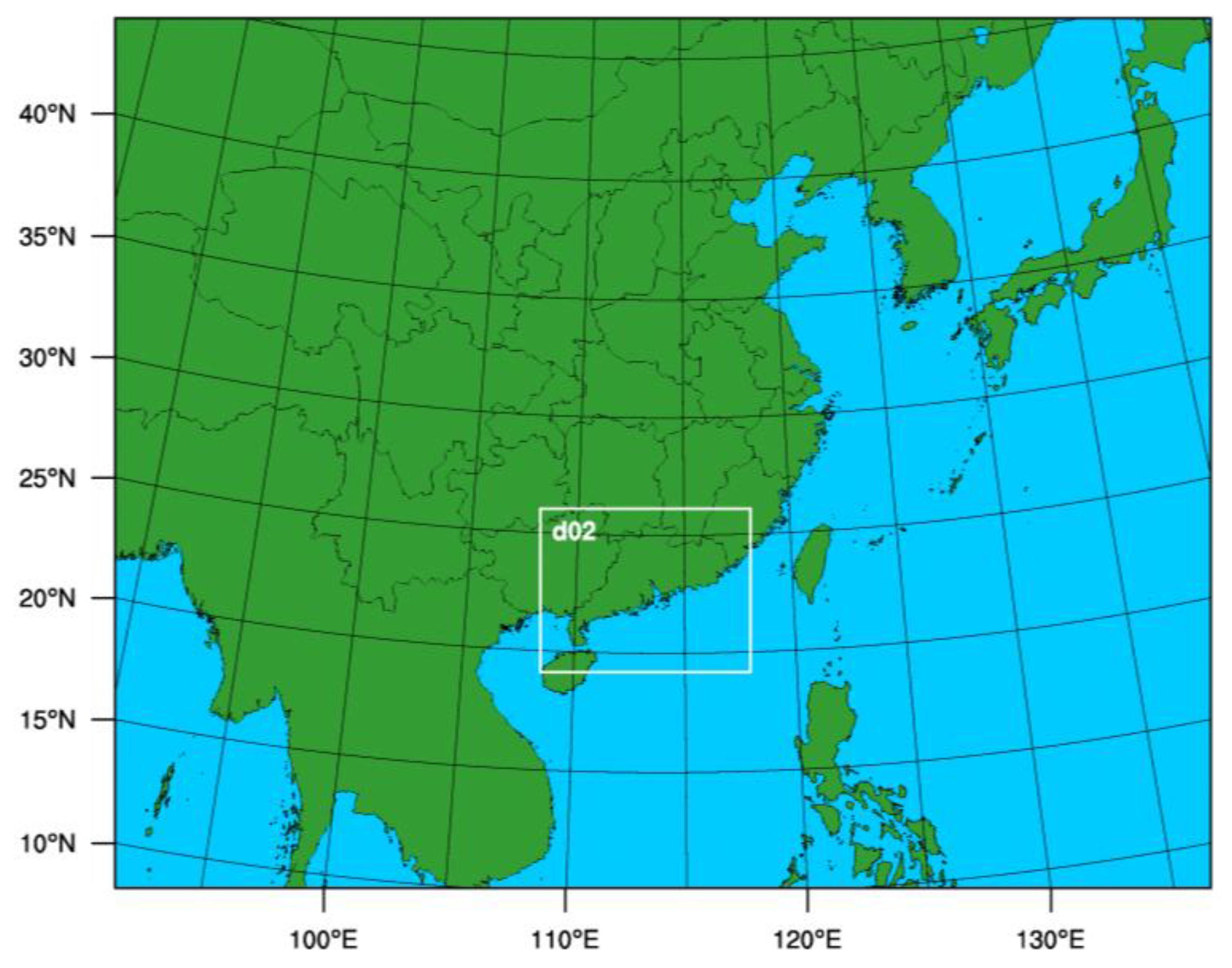
2.4. The WRF-Chem Model

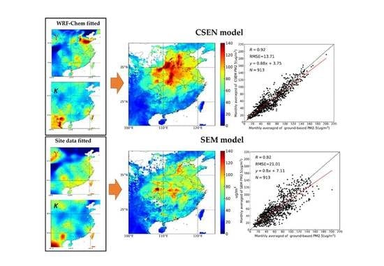
The horizontal resolution of 9 km for the parent domain area (90°E to 140°E, 10°N to 45°N) was set for the WRF-Chem model analysis. Moreover, the domain was set up with grid sizes of 188 × 149. Our current model settings cover most of China, including the surrounding terrestrial and oceanic areas (Figure 2). We obtained the emission inventory from the Multiresolution Emission Inventory for China (MEIC) and applied it with Final Operational Global Analysis (FNL) to run the WRF-Chem model in this research. The MEIC covers more than 700 anthropogenic sources of emissions in the Chinese mainland and contains five sectors (i.e., industry, power plant, transportation, residential combustion, and agricultural activity) and more than 10 major atmospheric pollutants, including SO₂, NOx, CO, NMVOC, NH₃, PM_2.5, PM₁₀, BC, OC, and carbon dioxide emissions [37]. For biogenic species, the Model of Emissions of Gas and Aerosols from Nature was used [38]. From the surface to the upper air limit of 50 hPa, there are 38 vertical layers, of which 12 layers are located below 2 km to sufficiently represent the vertical structure of the boundary layer. The model configuration and performance in the study domain can be found in our previous publication [30].

2.5. The CSEN Model

In the SEM, the parameters of aerosol characteristics (K and γ′) are generated based upon long-term observed data regression and have relatively low spatial and temporal resolutions. Therefore, it is difficult to establish a high-resolution PM_2.5 inversion with aerosol parameters based on a large-scale ground-based observation network. We can expect diminished model performance for the sites far from the ground-based observation sites.

To improve the SEM accuracy and evaluate the effect of aerosol characteristic variations, a new method for PM_2.5 estimation based upon coupling the SEM and the CTM was developed. As mentioned above, the CTM simulates both meteorological and aerosol chemical and physical effects based on an emission inventory. In this research, the WRF-Chem model was applied to provide simulated aerosol properties. As the WRF-Chem model uses emission information with high temporal and spatial resolutions driven by reasonable meteorology and basic chemistry, it is expected that the simulated overall aerosol property pattern is relatively more reliable compared to interpolation of site-based regression, although the uncertainty in absolute PM_2.5 mass concentration simulation at individual stations could be considerable.

Therefore, we first carried out a four-season simulation with WRF-Chem in this study. The model provides simultaneous data, including hourly ext, RH, and PM_2.5 concentrations at the same grid cells. Linear transformation of Equation (1) by log-transforming both sides at each grid cell, results in Equation (4) as follows:

$$ln\frac{ext}{P{M}_{2.5}}=lnK-{\gamma }^{\prime }ln\left(\frac{1-RH}{1-R{H}_0}\right)$$

(4)

which exactly satisfies a linear regression form as shown in Equation (5). γ′_(i,j) and K_(i,j) can be fitted by the slope and intercept from the linear regression at each model grid (i,j) since X_(i,j) and Y_(i,j) are the previously known values. Thus, γ′_(i,j) and K_(i,j) can be fitted by simultaneous measurements of ext _(i,j) RH_(i,j), and PM_2.5(i,j) mass at the same grid. The aerosol properties were derived once from each grid cell using the simulation of the individual months in this study.

$$Y_{\left(i,j\right)}=-{{\gamma }^{\prime }}_{\left(i,j\right)}·X_{\left(i,j\right)}+ln{K}_{\left(i,j\right)}$$

(5)

Thus, the gridded γ′and K parameters based on CTM data can be derived. Combining the observational ext and RH data, the PM_2.5 mass concentration can be evaluated by Equation (6) for the whole domain.

In summary, the spatial map of $ex{t}_{\left(i,j\right)}$ and $R{H}_{\left(i,j\right)}$ can be achieved by the interpolation of hourly $ex{t}_{\left(i,j\right)}$ and RH_(i,j) at GTS observational stations. Hour-specific AOD gridded data are retrieved from the MODIS satellite, and H is calculated and interpolated based on the observational visibility [24,25], while γ′ and K are gridded data estimated based on the WRF-Chem simulation for each grid cell and for each month. The temporal and spatial resolutions of the gridded γ′ and K could be further improved for downscaling issues.

$$P{M}_{2.5}{}_{\left(i,j\right)}=\frac{\frac{{\mathrm{AOD}}_{\left(i,j\right)}}{H_{\left(i,j\right)}}}{K_{\left(i,j\right)}\times {\left(\frac{1-R{H}_{\left(i,j\right)}}{1-R{H}_0}\right)}^{-{\gamma }_{\left(i,j\right)}^{\prime } }}$$

(6)

3. Results

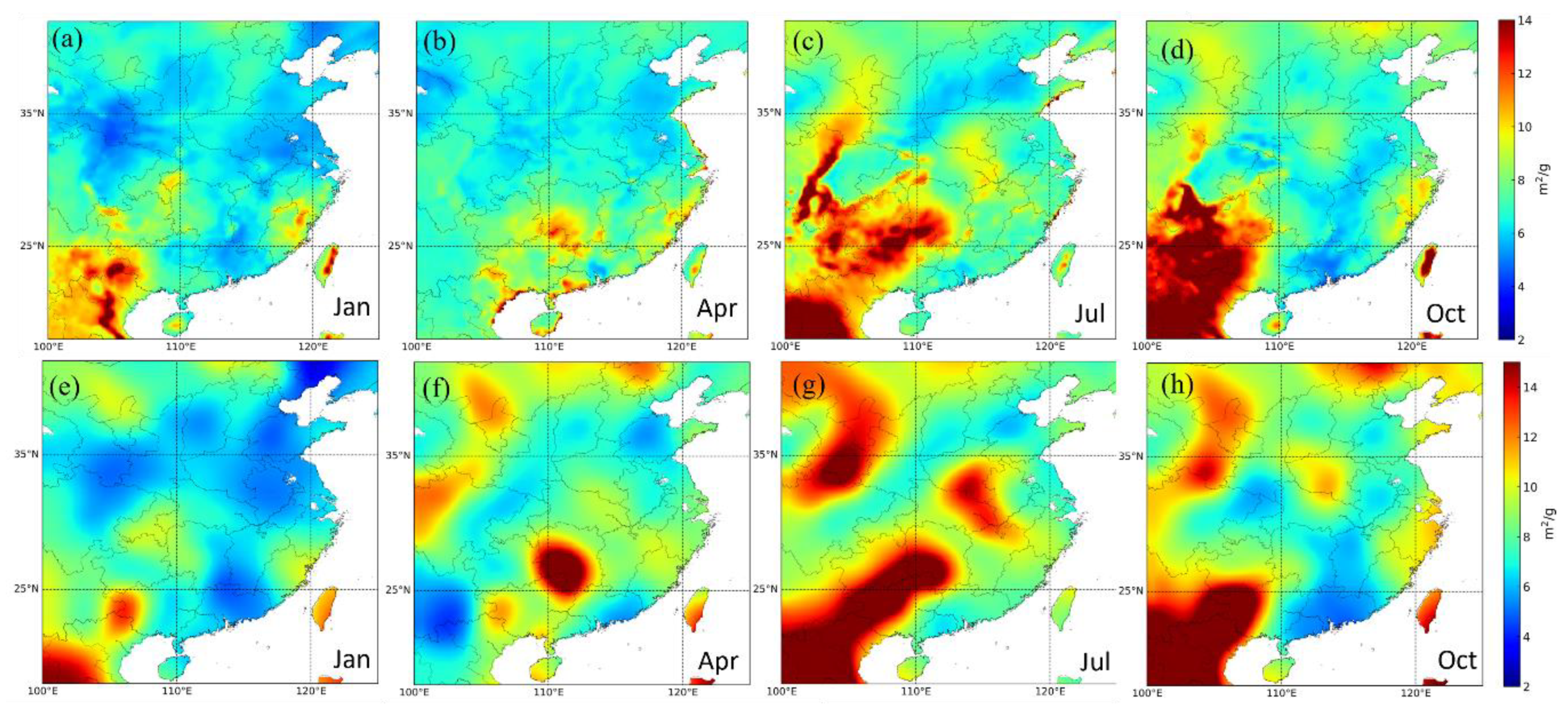
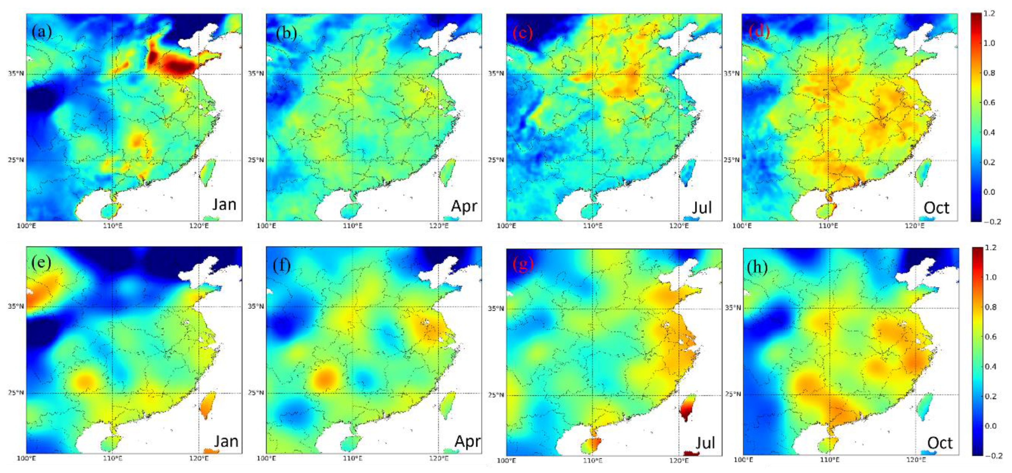
3.1. Evaluation of Aerosol Characteristics from WRF-Chem: γ′ and K

According to Equations (4) and (5), the two integrated parameters of aerosol properties can be derived by using the WRF-Chem data. The IHE of PM_2.5 explains how visibility deteriorates at a given PM_2.5 level if the air humidity is higher than normal, which reflects the dependence of the integrated light extinction ability of PM_2.5 on RH. γ′ is the coefficient of IHE. As demonstrated by Lin et al. (2015) [19], in addition to the RH dependence of the hygroscopic growth effect of aerosol, we also include the RH dependence on FMF and MEE factors, since the factors are also likely to depend on RH due to the variation in the aerosol characteristics in various meteorological conditions.

The results presented in Figure 3 show that the γ′ values are affected by both anthropogenic emissions and meteorological conditions. For the transition seasons (represented by October and April), the overall absolute levels and spatial pattern of γ′ from the SEM and WRF-Chem are similar, and the spatial pattern seems to be closely associated with emissions [39,40]. We observed higher values of γ′ in the eastern parts of China than in other regions. Guangxi, Jiangxi, Anhui, Shaanxi, Jiangsu, and Zhejiang were associated with significantly larger γ′ values than other areas, related to the significant industrial development in these areas in recent years. The lower values observed in the northern and central areas and the Tibetan Plateau in China are mainly due to higher dust or biomass burning aerosol loads [41], which are generally less hygroscopic than industrial aerosols [42]. A comparison of the two results shows that, although the spatial patterns are similar, the CTM results provide more details of the distribution of γ′ values at a much higher spatial resolution. However, regarding the spatial pattern in the winter and summer seasons (represented by January and July), the two γ′ results show considerable differences. Areas with the highest γ′ in winter in the CTM results are missing in the SEM results.

Regarding the seasonal variation in γ′ in the whole study domain, we observed generally higher γ′ values in most of the southern areas in October, generally higher γ′ values in most of the northern areas in July, the lowest γ′ values in the whole domain in spring, and a generally low γ′ background but highest γ′ values in specific areas, especially in JJJ (Beijing–Tianjin–Hebei) and Shandong Province in winter. Generally, the widely higher γ′ values in autumn and summer reflect the strong RH dependence of the IHE in the wet season, while a lower background of γ′ reflects the weaker RH dependence of the IHE in the dry season. Nevertheless, in specific regions, such as JJJ and Shandong Province, the IHE can be significantly influenced by meteorological conditions.

More specifically, the dry season (i.e., spring and winter) is usually marked by lower humidity, frequent cold fronts, and high wind speeds, which favor the formation of fugitive dust and its advection [43,44,45]. Because of this fugitive dust or dust storms, the average effective radius of particles in the dry season is larger, and the particles are generally less hygroscopic than the fine particles [44,45,46,47]. As a result, the lowest γ′ values in the whole domain occurred in spring, and a generally low γ′ background occurred in winter. The significantly high γ′ values were observed in the JJJ and Shandong areas in January, which should be related to the widely reported regional extreme haze events that frequently occur in the winter [48]. During these extreme haze events, in addition to the pollution accumulation due to stagnation and the significant decrease in the PBLH, abnormal southerly winds bring airmasses laden with pollutants and moisture. The extreme haze events result in an enhanced FMF, fine-mode effective radius, and volume concentration of PM_2.5 due to the hygroscopic growth effect of the particles and, after that, an increase in aerosol extinction and total AOD [43,44]. However, this significant hygroscopic effect associated with abnormal meteorological conditions, as shown in Figure 3a, cannot be reflected in the SEM results (Figure 3e), which is likely due to the low resolution and poor representation of the observation stations.

In spring (Figure 3b), the lowest γ′ might be associated with coarser particle generation, mainly due to the influence of more fugitive dust and dust storm events leading to a further decrease in aerosol hygroscopicity. During the wet season (i.e., summer and autumn), humid weather conditions are likely to be associated with a lower surface wind speed and sufficient humidity conditions conducive to the larger hygroscopic effect of aerosols. The higher γ′ values observed in the northern part than in the southern part of eastern China in summer (and vice versa in autumn) might be due to the variation in the relative abundance of precipitation.

K represents the integrated mass extinction efficiency, which is determined by the ratio of MEE and FMF [25]. As shown in Figure 4e–h, the MEE value is not sensitive to different scattering aerosol species [49]. Higher K values are observed in the southwest (Yunnan-Guizhou Plateau), northwest (Gansu), and some coastal areas located in eastern parts of China (i.e., Zhejiang), which are probably more affected by higher loading of coarse particles. The desertification in the Yunnan-Guizhou Plateau [50], the dust area in Gansu, and the increased sea salt aerosols in coastal areas may lead to a lower FMF [51] and thereafter a higher K value there. Overall, the spatial distribution patterns of the two models were comparable. However, a more detailed spatial distribution of K values was observed for the WRF-Chem results compared with the SEM in all seasons.

3.2. Validation of the Estimated PM_2.5

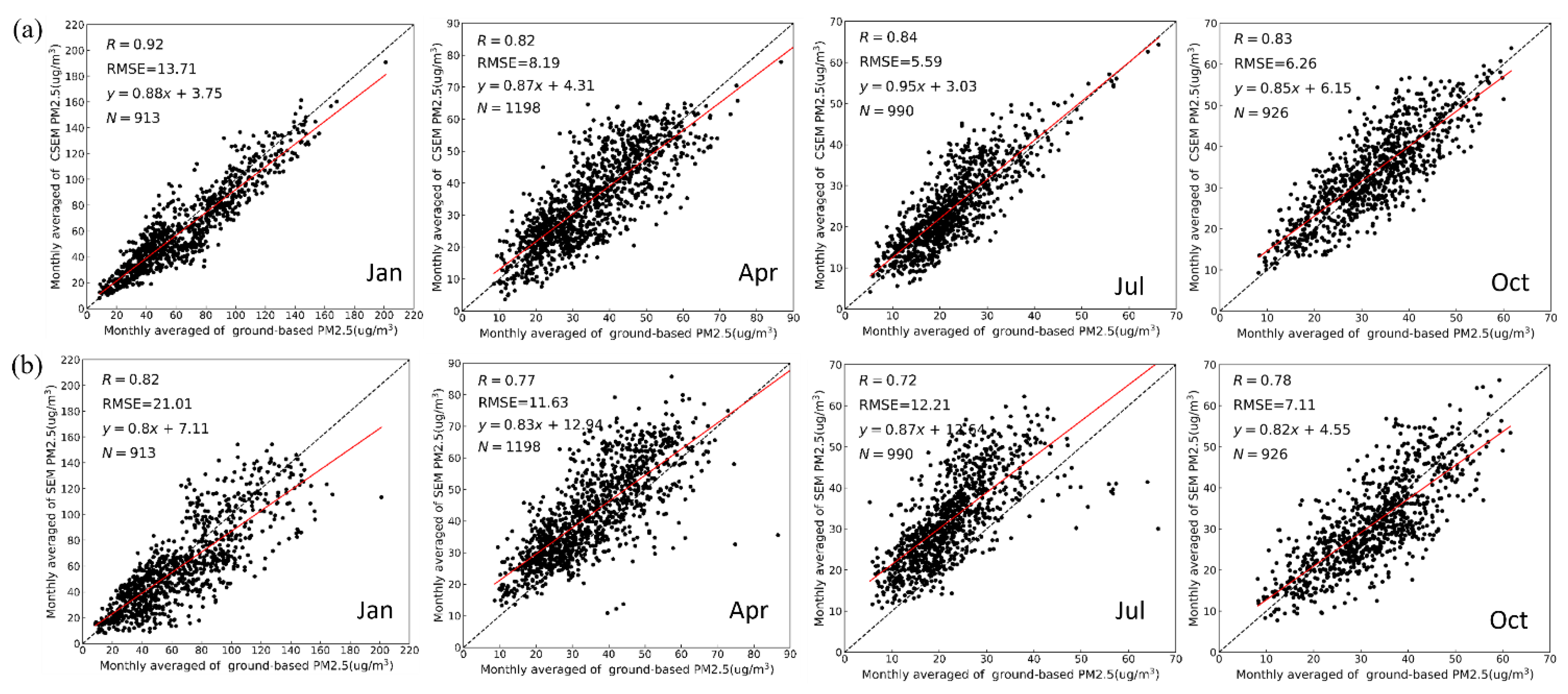
3.2.1. Statistical Results

All the daily PM_2.5 measurements from 1695 monitoring stations were used as validation to evaluate the CSEN model performance. Figure 5 shows the scatter plots between the observations and the estimated PM_2.5 mass concentrations of the CSEN and the SEM.

Based on the SEM method, the correlation coefficients (R) between the observed and estimated values were 0.82, 0.77, 0.75, and 0.78, with moderate biases (root mean square error (RMSE) = 21.01, 11.63, 12.21, and 7.11 μg/m³) for January, April, July, and October, respectively. For the CSEN method, on the other hand, the R values between the observed and estimated values were 0.92, 0.82, 0.84, and 0.83, with a much lower model bias (RMSE = 13.71, 8.19, 5.59, and 6.26 μg/m³) for January, April, July, and October, respectively. All the slopes based upon the CSEN model are closer to 1.

The mean absolute error (MAE) and mean relative error (MRE) between the predictions and observations for the four seasons were also calculated. The comparison of the four seasons of the two methods is shown in

Table 1. Comparison of the CSEN, SEM, and WRF-chem model performances.

Method	Month	R 1	RMSE 2 (µg/m3)	MAE 3 (µg/m3)	MRE 4 (%)
CSEN	Jan	0.92	13.71	8.56	10.22
	Apr	0.82	8.19	7.22	11.36
	Jul	0.84	5.59	4.65	12.29
	Oct.	0.83	6.26	5.71	15.88
SEM	Jan	0.8	21.01	21.11	21.32
	Apr	0.77	11.63	9.40	23.17
	Jul	0.72	12.21	10.03	37.32
	Oct.	0.72	7.11	6.83	20.15
WRF-chem	Jan	0.59	21.56	22.41	22.55
	Apr	0.67	13.25	11.21	23.94
	Jul	0.73	11.89	10.13	22.21
	Oct.	0.71	8.61	7.88	21.45

¹ Correlation coefficient; ² root mean square error; ³ mean absolute error; ⁴ mean relative error.

. Significant improvement in the PM_2.5 estimation by CSEN compared to that of SEM is clearly shown. In addition, both results are better than the CTM performance for PM_2.5 (the RMSE of January on average is greater than 21 µg/m³ and R is lower than 0.6 [30]).

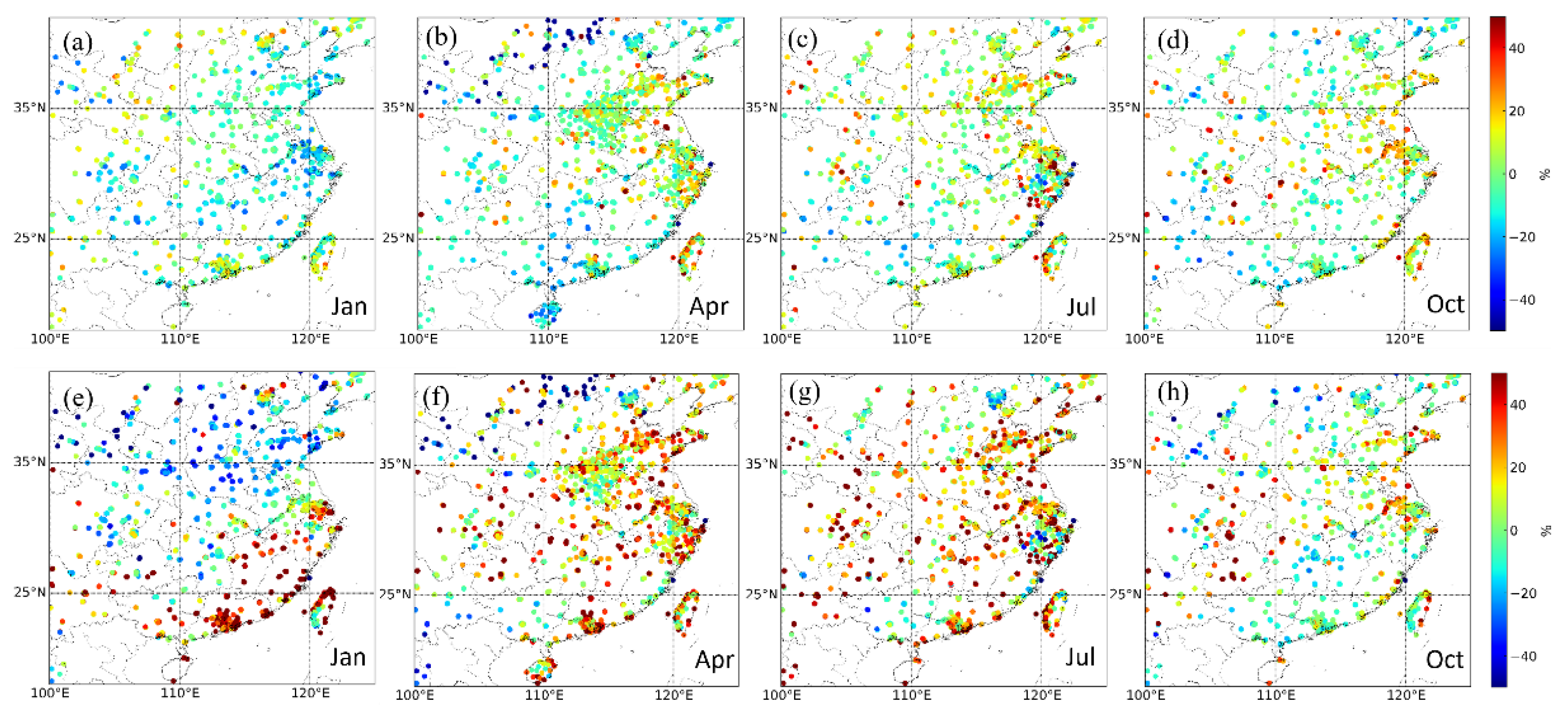
3.2.2. The Seasonal Variation in Spatial Distribution

The seasonal variations (represented by January, April, July, and October) in satellite-retrieved PM_2.5 with the corresponding near-surface observed data from all the sites in eastern China are shown in Figure 6. Here, the monthly averaged PM_2.5 estimation was calculated based on the result of the daily PM_2.5 estimation. The results show that the PM_2.5 levels are much higher in northern China than in other regions. According to the estimated results in Figure 6a–d, the PM_2.5 pollution still shows regional properties, as reported by previous studies [8,25]. Regional heating and the industrial sectors are mainly responsible for pollution episodes. The highest pollution levels occurred in winter, followed by autumn, spring, and summer. The modeling results in Figure 6a–h illustrate that the highest pollution levels are mainly concentrated in Northern China Plain (NCP) areas, consistent with the results from the ground-based monitoring stations (Figure 6i–l).

The PM_2.5 concentration levels estimated by the SEM method in the NCP areas significantly underestimated the observed concentration levels during winter. We also observed a severe overestimation of the SEM results for the same region during autumn. The CSEN model, on the other hand, provided a more robust result with higher levels of accuracy, especially in the major polluted area.

The spatial variation in the PM_2.5 deviation as a percentage between the evaluated PM_2.5 average and ground-based PM_2.5 average, including January, April, July, and October, is shown in Figure 7. PM_2.5 mass concentrations estimated by the CSEN model exhibit much smaller MRE values than those analyzed by SEM. The MRE values calculated for the ground-based monitoring stations were within the range from −50% to +50%, which were on average 30% smaller, especially during winter and summer.

Overall, significant improvements were observed in PM_2.5 estimations by the CSEN model specifically for January and July in terms of statistics and better spatial distribution patterns. This better agreement should be attributed to the significant difference in the estimated γ′ (especially in northern China) between WRF-Chem and the pure SEM method (Figure 3a–c). On the other hand, the better agreement, and the reduced biases in the validation results, especially in winter and summer, showed that the CTM γ′ in the CSEN method can provide more realistic aerosol properties, significantly improving model performance.

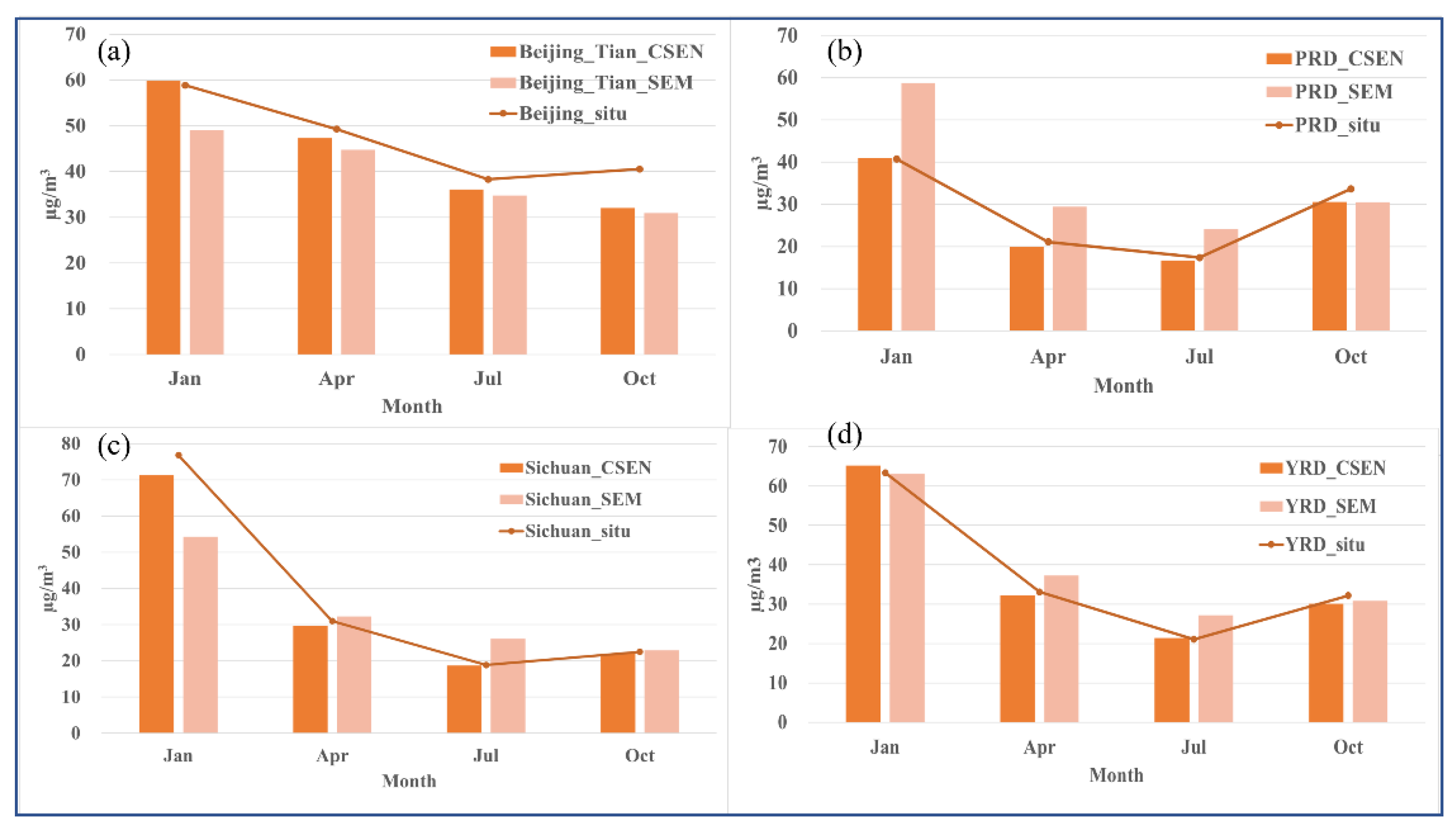
3.2.3. The Seasonal Variation in Major Clusters

To further explain the regional PM_2.5 mass concentration variations, we mainly focused on four key clusters in China: Beijing–Tianjin, YRD, Sichuan, and PRD (Figure 8 and

Table 2. Performance of the AOD–PM_2.5 algorithm with respect to the two methods in the four key urban clusters.

Region	Month	In Situ (µg/m3)	CSEN-MRE (%)	SEM-MRE (%)
Beijing–Tianjin	Jan	58.85	1.69	−16.70
	Apr	49.27	−3.97	−9.17
	Jul	38.27	−5.58	−9.11
	Oct.	40.53	−20.94	−23.71
PRD	Jan	40.71	0.59	44.32
	Apr	21.09	−5.44	39.57
	Jul	17.38	−3.86	38.76
	Oct.	33.64	−9.15	−9.33
Sichuan	Jan	76.80	−7.18	−29.33
	Apr	30.99	−3.93	4.05
	Jul	18.85	−0.82	38.25
	Oct.	22.49	−2.23	1.79
YRD	Jan	63.37	2.84	−0.49
	Apr	33.10	−2.61	12.57
	Jul	21.09	1.66	29.08
	Oct.	32.16	−6.36	−4.02

). According to Figure 8, the PM_2.5 concentrations retrieved by the two methods vary significantly among different regions. January was the most polluted month in all four critical urban clusters in China. In the Beijing–Tianjin area, the PM_2.5 concentrations dropped from 58.85 µg/m³ in January to 38.27 µg/m³ in July, increasing slightly to 40.53 µg/m³ in October. The mean PM_2.5 concentrations retrieved by the CSEN model performed better than those by the SEM in all four months, especially in January. On the other hand, neither model performed well in October, with MREs of −20.94% and −23.71%, respectively. In the PRD region, the mean PM_2.5 concentration retrieved by the SEM method is seriously overestimated, with MREs of 44.32%, 39.57%, and 38.76% in January, April, and July, respectively. In the Sichuan area, both methods underestimated the PM_2.5 concentration in January, although the CSEN provided a closer value to the ground-based monitoring stations. In the YRD region, the results from the CSEN method are slightly overestimated in January (2.84%) and July (1.66%) and underestimated in April (−2.61%) and October (−6.36%). In contrast, the results of the SEM are underestimated in January (−0.49%) and October (−4.02%) and overestimated in April (12.57%) and July (29.08%). The overall results obtained with the CSEN method provide more realistic values when compared with the ground-based monitoring network data in the four clusters.

4. Discussion and Conclusions

Large-scale high-resolution measurements of PM_2.5 are fundamental to investigating various environmental, climate, and adverse human health impacts. Although nationwide ground-based PM_2.5 monitoring networks are already implemented around China, limited by the nature of in situ observations, reaching high-resolution PM_2.5 retrievals at a larger scale is still challenging and hinders understanding the variability of PM_2.5 at different spatial scales. State-of-the-art statistical and machine learning models combining ground observations and satellite AOD have been applied to provide PM_2.5 estimation. However, most of these are limited in the physical understanding between the model inputs and outputs.

The physical-based SEM proposed in our previous study showed that the PM_2.5 estimation accuracy could be greatly improved by combining the aerosol characteristics into the physical model. In the SEM, the humidity coefficient (γ′) and an integrated reference value (K) of aerosol characteristics could be obtained based on matched in situ meteorological and air quality data, which are very sparse in spatial resolution and therefore limit the resolution of PM_2.5 estimation.

Therefore, in this research, we developed a new method for estimating surface PM_2.5 by coupling the SEM and a CTM-based numerical model (CSEN). The CSEN takes advantage of the WRF-Chem model in providing high spatial resolution of aerosol properties to optimize the aerosol parameters (γ′ and K) required for the PM_2.5 estimation. Four months of air quality were simulated with the WRF-Chem model to acquire the variation in aerosol property parameters (γ′ and K).

Comparison of γ′ values and K values between the two methods show that their overall spatial patterns are comparable, but the new method exhibits a significantly improved resolution, and there is a significant difference in the γ′ values in winter and summer. Validation results indicated that the correlation coefficient between the observed and the estimated values increased to 0.92, 0.82, 0.84, and 0.83 with a much lower model bias by CSEN, from 0.82, 0.77, 0.75, and 0.78, with a moderate bias by SEM for January, April, July, and October, respectively. In addition, the RMSE was reduced by between 0.85 and 7.3 µg/m³.

The CSEN PM_2.5 estimation is significantly improved in all seasons, especially in winter and summer, which is because the CTM provides a more complete and more realistic spatial distribution of aerosol properties with emission data at high spatial-temporal resolution based on reasonable meteorology. However, the uncertainty in the absolute PM_2.5 concentration simulated at individual stations could be primarily due to the existing model errors and uncertainties. The results prove that CSEN is valuable for PM_2.5 evaluation at urban and regional scales, especially for regions lacking ground measurements. It also provides valuable tactics for air pollution control strategies and health risk assessment tactics.

Limitations remain in CSEN estimation mainly due to the following: (1) In this work, we did not fill pixel gaps of AOD due to the existence of thick clouds, which might reduce the model performance at these pixels. (2) The number of PM_2.5 observed stations was limited, and the PM_2.5 observation stations were irregularly distributed, which might reduce the performance of the model far from the monitoring station area. (3) Although the results show that the CTM could provide a reasonably high spatial–temporal resolution for γ′ and K values driven by emission and meteorology, the spatial resolution and accuracy of meteorological field and aerosol parameters simulated by the WRF-Chem model are still affected by model errors and uncertainties, which could be further improved by, for example, more reliable parameterization schemes for the formation and the gas-particle conversion of secondary aerosols. (4) The γ′ and K were fitted by one-month simulations in this study to acquire the local average aerosol properties. The daily and synoptic scale variation in aerosol properties due to the transport impact and abrupt emission variation could be smoothed by using monthly period regression.

References

1. van Donkelaar, A.; Martin, R.V.; Park, R.J. Estimating ground-level PM2.5 using aerosol optical depth determined from satellite remote sensing. J. Geophys. Res. Atmos. 2006, 111, D2. [Google Scholar] [CrossRef]
2. Bao, F.W.; Li, Y.; Cheng, T.H.; Gao, J.H.; Yuan, S.Y. Estimating the Column Concentrations of Black Carbon Aerosols in China Using MODIS Products. Environ. Sci. Technol. 2020, 54, 11025–11036. [Google Scholar] [CrossRef] [PubMed]
3. Alexeeff, S.E.; Schwartz, J.; Kloog, I.; Chudnovsky, A.; Koutrakis, P.; Coull, B.A. Consequences of kriging and land use regression for PM2.5 predictions in epidemiologic analyses: Insights into spatial variability using high-resolution satellite data. J. Exp. Sci. Environ. Epidemiol. 2015, 25, 138–144. [Google Scholar] [CrossRef] [PubMed] [Green Version]
4. Brauer, M.; Freedman, G.; Frostad, J.; van Donkelaar, A.; Martin, R.V.; Dentener, F.; van Dingenen, R.; Estep, K.; Amini, H.; Apte, J.S.; et al. Ambient Air Pollution Exposure Estimation for the Global Burden of Disease 2013. Environ. Sci. Technol. 2016, 50, 79–88. [Google Scholar] [CrossRef] [PubMed]
5. Pope, C.A., 3rd; Burnett, R.T.; Turner, M.C.; Cohen, A.; Krewski, D.; Jerrett, M.; Gapstur, S.M.; Thun, M.J. Lung cancer and cardiovascular disease mortality associated with ambient air pollution and cigarette smoke: Shape of the exposure-response relationships. Environ. Health Perspect. 2011, 119, 1616–1621. [Google Scholar] [CrossRef] [PubMed] [Green Version]
6. Tie, X.X.; Wu, D.; Brasseur, G. Lung cancer mortality and exposure to atmospheric aerosol particles in Guangzhou, China. Atmos. Environ. 2009, 43, 2375–2377. [Google Scholar] [CrossRef]
7. Wong, N.S.; Leung, C.C.; Li, Y.; Poon, C.M.; Yao, S.; Wong, E.L.Y.; Lin, C.; Lau, A.K.H.; Lee, S.S. PM2·5 concentration and elderly tuberculosis: Analysis of spatial and temporal associations. Lancet 2017, 390, S68. [Google Scholar] [CrossRef]
8. Lin, C.; Li, Y.; Lau, A.K.H.; Deng, X.; Tse, T.K.T.; Fung, J.C.H.; Li, C.; Li, Z.; Lu, X.; Zhang, X.; et al. Estimation of long-term population exposure to PM2.5 for dense urban areas using 1-km MODIS data. Remote Sens. Environ. 2016, 179, 13–22. [Google Scholar] [CrossRef] [Green Version]
9. Chu, Y.Y.; Liu, Y.S.; Li, X.Y.; Liu, Z.Y.; Lu, H.S.; Lu, Y.A.; Mao, Z.F.; Chen, X.; Li, N.; Ren, M.; et al. A Review on Predicting Ground PM2.5 Concentration Using Satellite Aerosol Optical Depth. Atmosphere 2016, 7, 129. [Google Scholar] [CrossRef] [Green Version]
10. He, B.H.Q.; Heal, M.R.; Reis, S. Land-Use Regression Modelling of Intra-Urban Air Pollution Variation in China: Current Status and Future Needs. Atmosphere 2018, 9, 134. [Google Scholar] [CrossRef] [Green Version]
11. Kaufman, Y.J.; Tanre, D.; Boucher, O. A satellite view of aerosols in the climate system. Nature 2002, 419, 215–223. [Google Scholar] [CrossRef] [PubMed]
12. Li, Y.; Yuan, S.; Fan, S.; Song, Y.; Wang, Z.; Yu, Z.; Yu, Q.; Liu, Y. Satellite Remote Sensing for Estimating PM2.5 and Its Component. Curr. Pollut. Rep. 2021, 7, 72–87. [Google Scholar] [CrossRef]
13. Shin, M.; Kang, Y.; Park, S.; Im, J.; Yoo, C.; Quackenbush, L.J. Estimating ground-level particulate matter concentrations using satellite-based data: A review. GISci. Remote Sens. 2020, 57, 174–189. [Google Scholar] [CrossRef]
14. Danesh Yazdi, M.; Kuang, Z.; Dimakopoulou, K.; Barratt, B.; Suel, E.; Amini, H.; Lyapustin, A.; Katsouyanni, K.; Schwartz, J. Predicting fine particulate matter (PM2.5) in the greater london area: An ensemble approach using machine learning methods. Remote Sens. 2020, 12, 914. [Google Scholar] [CrossRef] [Green Version]
15. Guo, Y.X.; Tang, Q.H.; Gong, D.Y.; Zhang, Z.Y. Estimating ground-level PM2.5 concentrations in Beijing using a satellite-based geographically and temporally weighted regression model. Remote Sens. Environ. 2017, 198, 140–149. [Google Scholar] [CrossRef]
16. Hua, Z.Q.; Sun, W.W.; Yang, G.; Du, Q. A Full-Coverage Daily Average PM2.5 Retrieval Method with Two-Stage IVW Fused MODIS C6 AOD and Two-Stage GAM Model. Remote Sen. 2019, 11, 1558. [Google Scholar] [CrossRef] [Green Version]
17. Park, S.; Lee, J.; Im, J.; Song, C.K.; Choi, M.; Kim, J.; Lee, S.; Park, R.; Kim, S.M.; Yoon, J.; et al. Estimation of spatially continuous daytime particulate matter concentrations under all sky conditions through the synergistic use of satellite-based AOD and numerical models. Sci. Total Environ. 2020, 713, 136516. [Google Scholar] [CrossRef]
18. Xue, T.; Zheng, Y.; Tong, D.; Zheng, B.; Li, X.; Zhu, T.; Zhang, Q. Spatiotemporal continuous estimates of PM2.5 concentrations in China, 2000-2016: A machine learning method with inputs from satellites, chemical transport model, and ground observations. Environ. Int. 2019, 123, 345–357. [Google Scholar] [CrossRef]
19. Lin, C.Q.; Li, Y.; Yuan, Z.B.; Lau, A.K.H.; Li, C.C.; Fung, J.C.H. Using satellite remote sensing data to estimate the high-resolution distribution of ground-level PM2.5. Remote Sens. Environ. 2015, 156, 117–128. [Google Scholar] [CrossRef]
20. Xue, Y.; Li, Y.; Guang, J.; Tugui, A.; She, L.; Qin, K.; Fan, C.; Che, Y.H.; Xie, Y.Q.; Wen, Y.N.; et al. Hourly PM2.5 Estimation over Central and Eastern China Based on Himawari-8 Data. Remote Sen. 2020, 12, 855. [Google Scholar] [CrossRef] [Green Version]
21. Zhang, K.N.; de Leeuw, G.; Yang, Z.Q.; Chen, X.F.; Su, X.L.; Jiao, J.S. Estimating Spatio-Temporal Variations of PM2.5 Concentrations Using VIIRS-Derived AOD in the Guanzhong Basin, China. Remote Sens. 2019, 11, 2679. [Google Scholar] [CrossRef] [Green Version]
22. Chu, D.A.; Tsai, T.C.; Chen, J.P.; Chang, S.C.; Jeng, Y.J.; Chiang, W.L.; Lin, N.H. Interpreting aerosol lidar profiles to better estimate surface PM2.5 for columnar AOD measurements. Atmos. Environ. 2013, 79, 172–187. [Google Scholar] [CrossRef]
23. Emili, E.; Popp, C.; Petitta, M.; Riffler, M.; Wunderle, S.; Zebisch, M. PM10 remote sensing from geostationary SEVIRI and polar-orbiting MODIS sensors over the complex terrain of the European Alpine region. Remote Sens. Environ. 2010, 114, 2485–2499. [Google Scholar] [CrossRef]
24. Koelemeijer, R.B.A.; Homan, C.D.; Matthijsen, J. Comparison of spatial and temporal variations of aerosol optical thickness and particulate matter over Europe. Atmos. Environ. 2006, 40, 5304–5315. [Google Scholar] [CrossRef]
25. Li, Y.; Lin, C.Q.; Lau, A.K.H.; Liao, C.H.; Zhang, Y.B.; Zeng, W.T.; Li, C.C.; Fung, J.C.H.; Tse, T.K.T. Assessing Long-Term Trend of Particulate Matter Pollution in the Pearl River Delta Region Using Satellite Remote Sensing. Environ. Sci. Technol. 2015, 49, 11670–11678. [Google Scholar] [CrossRef] [PubMed]
26. Schaap, M.; Apituley, A.; Timmermans, R.M.A.; Koelemeijer, R.B.A.; de Leeuw, G. Exploring the relation between aerosol optical depth and PM2.5 at Cabauw, the Netherlands. Atmos. Chem. Phys. 2009, 9, 909–925. [Google Scholar] [CrossRef] [Green Version]
27. Tao, J.H.; Zhang, M.G.; Chen, L.F.; Wang, Z.F.; Su, L.; Ge, C.; Han, X.; Zou, M.M. A method to estimate concentrations of surface-level particulate matter using satellite-based aerosol optical thickness. Sci. China Earth Sci. 2013, 56, 1422–1433. [Google Scholar] [CrossRef]
28. Liu, Y.; Park, R.J.; Jacob, D.J.; Li, Q.B.; Kilaru, V.; Sarnat, J.A. Mapping annual mean ground-level PM2.5 concentrations using Multiangle Imaging Spectroradiometer aerosol optical thickness over the contiguous United States. J. Geophys. Res. Atmos. 2004, 109, D22206. [Google Scholar]
29. van Donkelaar, A.; Martin, R.V.; Brauer, M.; Kahn, R.; Levy, R.; Verduzco, C.; Villeneuve, P.J. Global estimates of ambient fine particulate matter concentrations from satellite-based aerosol optical depth: Development and application. Environ. Health Perspect. 2010, 118, 847–855. [Google Scholar] [CrossRef] [Green Version]
30. Gao, J.; Li, Y.; Zhu, B.; Hu, B.; Wang, L.; Bao, F. What have we missed when studying the impact of aerosols on surface ozone via changing photolysis rates? Atmos. Chem. Phys. 2020, 20, 10831–10844. [Google Scholar] [CrossRef]
31. Tie, X.; Geng, F.; Guenther, A.; Cao, J.; Greenberg, J.; Zhang, R.; Apel, E.; Li, G.; Weinheimer, A.; Chen, J.; et al. Megacity impacts on regional ozone formation: Observations and WRF-Chem modeling for the MIRAGE-Shanghai field campaign. Atmos. Chem. Phys. 2013, 13, 5655–5669. [Google Scholar] [CrossRef] [Green Version]
32. Zhang, H.; DeNero, S.P.; Joe, D.K.; Lee, H.H.; Chen, S.H.; Michalakes, J.; Kleeman, M.J. Development of a source oriented version of the WRF/Chem model and its application to the California regional PM10/PM2.5 air quality study. Atmos. Chem. Phys. 2014, 14, 485–503. [Google Scholar] [CrossRef] [Green Version]
33. Hu, X.M.; Xue, M.; Kong, F.Y.; Zhang, H.L. Meteorological Conditions During an Ozone Episode in Dallas-Fort Worth, Texas, and Impact of Their Modeling Uncertainties on Air Quality Prediction. J. Geophys. Res. Atmos. 2019, 124, 1941–1961. [Google Scholar] [CrossRef]
34. Gao, M.; Han, Z.W.; Liu, Z.R.; Li, M.; Xin, J.Y.; Tao, Z.N.; Li, J.W.; Kang, J.E.; Huang, K.; Dong, X.Y.; et al. Air quality and climate change, Topic 3 of the Model Inter-Comparison Study for Asia Phase III (MICS-Asia III)—Part 1: Overview and model evaluation. Atmos. Chem. Phys. 2018, 18, 4859–4884. [Google Scholar] [CrossRef] [Green Version]
35. Gao, J.H.; Zhu, B.; Xiao, H.; Kang, H.Q.; Pan, C.; Wang, D.D.; Wang, H.L. Effects of black carbon and boundary layer interaction on surface ozone in Nanjing, China. Atmos. Chem. Phys. 2018, 18, 7081–7094. [Google Scholar] [CrossRef] [Green Version]
36. Liu, Y.; Sarnat, J.A.; Kilaru, V.; Jacob, D.J.; Koutrakis, P. Estimating ground-level PM2.5 in the eastern United States using satellite remote sensing. Environ. Sci. Technol. 2005, 39, 3269–3278. [Google Scholar] [CrossRef] [Green Version]
37. Li, M.; Zhang, Q.; Kurokawa, J.; Woo, J.H.; He, K.B.; Lu, Z.F.; Ohara, T.; Song, Y.; Streets, D.G.; Carmichael, G.R.; et al. MIX: A mosaic Asian anthropogenic emission inventory under the international collaboration framework of the MICS-Asia and HTAP. Atmos. Chem. Phys. 2017, 17, 935–963. [Google Scholar] [CrossRef] [Green Version]
38. Guenther, A.; Karl, T.; Harley, P.; Wiedinmyer, C.; Palmer, P.I.; Geron, C. Estimates of global terrestrial isoprene emissions using MEGAN (Model of Emissions of Gases and Aerosols from Nature). Atmos. Chem. Phys. 2006, 6, 3181–3210. [Google Scholar] [CrossRef] [Green Version]
39. Zheng, G.J.; Duan, F.K.; Su, H.; Ma, Y.L.; Cheng, Y.; Zheng, B.; Zhang, Q.; Huang, T.; Kimoto, T.; Chang, D.; et al. Exploring the severe winter haze in Beijing: The impact of synoptic weather, regional transport and heterogeneous reactions. Atmos. Chem. Phys. 2015, 15, 2969–2983. [Google Scholar] [CrossRef] [Green Version]
40. Elser, M.; Huang, R.-J.; Wolf, R.; Slowik, J.G.; Wang, Q.; Canonaco, F.; Li, G.; Bozzetti, C.; Daellenbach, K.R.; Huang, Y.; et al. New insights into PM2.5 chemical composition and sources in two major cities in China during extreme haze events using aerosol mass spectrometry. Atmos. Chem. Phys. 2016, 16, 3207–3225. [Google Scholar] [CrossRef] [Green Version]
41. He, Q.S.; Zhou, G.Q.; Geng, F.H.; Gao, W.; Yu, W. Spatial distribution of aerosol hygroscopicity and its effect on PM2.5 retrieval in East China. Atmos. Res. 2016, 170, 161–167. [Google Scholar] [CrossRef]
42. Zhang, K.Q.; Ma, Y.J.; Xin, J.Y.; Liu, Z.R.; Ma, Y.N.; Gao, D.D.; Wu, J.S.; Zhang, W.Y.; Wang, Y.S.; Shen, P.K. The aerosol optical properties and PM2.5 components over the world’s largest industrial zone in Tangshan, North China. Atmos. Res. 2018, 201, 226–234. [Google Scholar] [CrossRef]
43. Liu, X.G.; Li, J.; Qu, Y.; Han, T.; Hou, L.; Gu, J.; Chen, C.; Yang, Y.; Liu, X.; Yang, T.; et al. Formation and evolution mechanism of regional haze: A case study in the megacity Beijing, China. Atmos. Chem. Phys. 2013, 13, 4501–4514. [Google Scholar] [CrossRef] [Green Version]
44. Yang, Y.; Liu, X.; Qu, Y.; Wang, J.; An, J.; Zhang, Y.; Zhang, F. Formation mechanism of continuous extreme haze episodes in the megacity Beijing, China, in January 2013. Atmos. Res. 2015, 155, 192–203. [Google Scholar] [CrossRef]
45. Zamora, M.L.; Peng, J.; Hu, M.; Guo, S.; Marrero-Ortiz, W.; Shang, D.; Zheng, J.; Du, Z.; Wu, Z.; Zhang, R. Wintertime aerosol properties in Beijing. Atmos. Chem. Phys. 2019, 19, 14329–14338. [Google Scholar] [CrossRef] [Green Version]
46. Zhang, M.; Jin, S.; Ma, Y.; Fan, R.; Wang, L.; Gong, W.; Liu, B. Haze events at different levels in winters: A comprehensive study of meteorological factors, Aerosol characteristics and direct radiative forcing in megacities of north and central China. Atmos. Environ. 2021, 245, 118056. [Google Scholar] [CrossRef]
47. Ma, N.; Zhao, C.; Chen, J.; Xu, W.; Yan, P.; Zhou, X. A novel method for distinguishing fog and haze based on PM2.5, visibility, and relative humidity. Sci. China Earth Sci. 2014, 57, 2156–2164. [Google Scholar] [CrossRef]
48. Chen, J.; Li, Z.; Lv, M.; Wang, Y.; Wang, W.; Zhang, Y.; Wang, H.; Yan, X.; Sun, Y.; Cribb, M. Aerosol hygroscopic growth, contributing factors, and impact on haze events in a severely polluted region in northern China. Atmos. Chem. Phys. 2019, 19, 1327–1342. [Google Scholar] [CrossRef] [Green Version]
49. Jung, C.H.; Lee, J.Y.; Kim, Y.P. Multicomponent aerosol mass efficiency with various mixture types for polydispersed aerosol. Part. Sci. Technol. 2018, 36, 857–866. [Google Scholar] [CrossRef]
50. Hong, L.; Huang, Y.; Peng, S. Monitoring the trends of water-erosion desertification on the Yunnan-Guizhou Plateau, China from 1989 to 2016 using time-series Landsat images. PLoS ONE 2020, 15, e0227498. [Google Scholar] [CrossRef]
51. Zhu, J.; Xia, X.; Che, H.; Wang, J.; Zhang, J.; Duan, Y. Study of aerosol optical properties at Kunming in southwest China and long-range transport of biomass burning aerosols from North Burma. Atmos. Environ. 2016, 169, 237–247. [Google Scholar] [CrossRef]
Figure 1. (a) Spatial distribution of PM2.5 monitoring sites (AQMS) included in this research (the red dots indicate the sites for calibration, and the green dots indicate the sites for validation). (b) Spatial distribution of meteorological data monitoring sites (GTS) included in this research.
Remotesensing 14 02360 g001
Figure 2. The WRF-Chem model domain setting and location.
Remotesensing 14 02360 g002
Figure 3. Monthly spatial distribution of aerosol characteristics γ′, (ad) are derived from WRF-Chem model data; (eh) are derived from SEM.
Remotesensing 14 02360 g003
Figure 4. Monthly spatial distribution of aerosol characteristics (K): (ad) are fitted by WRF-Chem model parameters; (eh) are fitted by station meteorological parameters.
Remotesensing 14 02360 g004
Figure 5. Spatial correlation coefficients between the monthly (January, April, July, and October) average of the evaluated PM2.5 average and ground-based PM2.5 are estimated ((a) CSEN; (b) SEM).
Remotesensing 14 02360 g005
Figure 6. Spatial distributions of PM2.5 in January, April, July, and October as modeled by the SEM and CSEN models. ((ad) CSEN; (eh) SEM; (il) site observations).
Remotesensing 14 02360 g006
Figure 7. The monthly normalized bias of the estimated PM2.5 average with the ground-based PM2.5 average ((ad) MRE of PM2.5 by CSEN; (eh) MRE of PM2.5 by SEM).
Remotesensing 14 02360 g007
Figure 8. Comparison of the monthly average PM2.5 concentration evaluated by CSEN and SEM with ground-observed data in (a) Beijing–Tianjin, (b) PRD, (c) Sichuan, and (d) YRD.
Remotesensing 14 02360 g008