Abstract
Off-channel areas are one of the most impacted aquatic habitats by humans globally, as extensive agricultural and urban development has limited them to roughly 10% of historical extent. This is also true for California’s Sacramento River Valley, where historically frequent widespread inundation has been reduced to a few off-channel water bodies along the mid-Sacramento River. This remaining shallow-water habitat provides crucial ecological benefits to multiple avian and fish species, but especially to floodplain-adapted species such as Chinook salmon (Oncorhynchus tshawytscha). Characterizing spatiotemporal off-channel dynamics, including inundation extent and residence time, is fundamental to better understanding the intrinsic value of such habitats and their potential to support recovery actions. Remote sensing techniques have been increasingly used to map surface water at regional and local scales, with improved resolutions. As such, this study maps off-channel inundation areas and describes their temporal dynamics by analyzing pixel-based time- series of multiple water indices, modified Normalized Difference Water Index (mNDWI) and the Automated Water Extraction Index (AWEI), generated from LandSat-8 and Sentinel-2 data between 2013–2021. Quantified off-channel area was similar with each water index and method used, but improved performance was associated with Sentinel-2 products and AWEI index to identify wetted areas under lower mainstem discharges. Results indicate an uneven distribution of off-channel habitat in the study area, with limited inundated areas in upstream reaches (<16% of total off-channel area for greater flows). In addition, much less habitat exists for flows under 400 m3/s, an important migration cue for endangered winter-run Chinook salmon, limiting juvenile access to areas with enhanced rearing conditions. Off-channel habitat residence times averaged between 7 and 16 days, primarily defined by the rate of receding flows, with rapid flow recession providing marginal off-channel habitat. This study shows reasonable performance of moderate resolution LandSat-8 and Sentinel-2 remote sensing imagery to characterize shallow-water inundated habitat in higher-order rivers, and as a method to inform restoration and native fish recovery efforts.
1. Introduction
Geomorphic processes form and maintain shallow-water inundated habitats on channel margins of actively meandering rivers [1,2]. These habitats, which increase channel complexity and serve critical ecological functions, are generated from the inundation of historical, often disconnected, channels (e.g., oxbow lakes), overbank flows (e.g., floodplains), and point bar dynamics (e.g., scour channels on point bars). They support essential parts of riverine ecosystems that provide habitat and nutrients for terrestrial and aquatic animals [3,4,5,6]. They are among the most productive environments, supporting high biodiversity, enhancing trophic resources, and increasing residence time compared with mainstem rivers [3,5,7,8,9]. The ecological importance of off-channel habitats is reflected in the evolution of numerous life history strategies, including those of numerous native fishes [3,10,11,12,13].
Off-channel habitats also are highly impacted by humans globally [14]. Approximately 90% of Europe’s and North America’s shallow-water areas have been developed, primarily for agriculture and urban use [5]. As such, disconnections between mainstem and adjacent floodplains have altered geofluvial processes, riverine productivity, and aquatic community structure, especially for floodplain-adapted species [15]. In California, USA, the Sacramento River once flooded the Sacramento Valley frequently, creating extensive seasonal shallow-water habitat (“inland sea”) that benefited multiple fishes and avian species [16]. California’s water infrastructure development greatly reduced the frequency and extent of off-channel inundation by flow regulation and levee construction. Currently, only 5% of historical floodplains remain in the Sacramento Valley, mostly within managed flood bypasses (Yolo and Sutter bypasses) that divert water during high-flow events [17]. Occasional flooding of such areas provides increases in shallow-water habitat during some years, but these bypasses were developed in the lower Sacramento River valley exclusively. In contrast, the middle Sacramento River, between Red Bluff and Colusa, generally lack the same type of periodic expansion of shallow-water habitat, instead containing a mosaic of off-channel habitats such as oxbow lakes, scour channels, and side pools, denoted as off-channel water bodies (OCWB) [18]. They provide critical habitat for Western Pond turtle (Clemmys marmorata), Sacramento pikeminnow (Ptychochelilus grandis), and Sacramento sucker (Catostomus occidentalis) [19,20]. The middle Sacramento River is also an important migratory corridor for juvenile salmonids, and OCWB’s shallow-water habitats provide important growth opportunities for salmonid fry [21,22]. Enhanced growth can promote higher rates of survival for juvenile salmonids during their remaining freshwater life stages [23]. Furthermore, anadromous fishes with greater body mass at ocean entry are associated with higher adult return rates [24]. Thus, such habitats are critical to the recovery of numerous native species listed under the Endangered Species Act, including the iconic winter-run Chinook salmon, which is endemic to the Sacramento River [23,25,26].
Despite their importance, comprehensive and consistent datasets on the range and availability of OCWBs along the middle Sacramento River are lacking [23]. Identifying ways to estimate OCWB dynamics, expanding our knowledge of their ecological use as a function of mainstem flow, habitat capacity, and residence times is of paramount importance. Such information would help managers and decision-makers develop recovery actions targeting juvenile salmonids in these areas, such as defining flow pulses and landform changes to expand shallow-water habitat, while reducing stranding risk, during low-flow years [18]. Incorporating this information in juvenile production models (e.g., WRHAP) [23] and/or decision-making models (e.g., winter-run DSM) [27] can also improve estimates of population response to proposed actions.
Advances in remote sensing imagery and geographic information systems (GIS) allowed the spatiotemporal analysis of eco-hydrological features in regions and river basins of interest (e.g., North Pacific Rim) [28]. Extensive literature exists on using these technologies for inundation modeling [29,30,31,32,33,34], flood monitoring [35,36,37], river geomorphology [38,39], habitat mosaic shifting [40], and assessment of in-stream and floodplain habitats [13,28,41,42,43,44,45,46]. Such analyses have been performed at a wide range of spatial resolutions, from fine (≤5 m; Quickbird) to moderate (10 to 100 m; Sentinel-2 imagery), depending on study area extent and required level of detail. The interpretation of these river features can be limited by satellite imagery’s ability to resolve temporal changes in river features from relatively coarse overpass frequency (~8 days for LandSat) [47]. However, the relative abundance and representation of major habitat characteristics in dynamic river systems is relatively stable even as the mosaic of habitats changes through time [48,49]. As such, multitemporal satellite remote sensing products can be used to describe and compare the abundance and distribution of the shifting mosaic of shallow inundated habitat [28,50]. Most studies using these products focus on estimating off-channel habitat characteristics such as physical complexity [45], extension, width, or type of riverine habitat (e.g., orthofluvial vs. parafluvial zones) [41]. For instance, a comprehensive geospatial database based on global Landsat TM imagery (30 m resolution), the Riverscape Analysis Project (RAP), described the distribution and physical characteristics of river basins, floodplains, and river networks for catchments draining into the North Pacific, including the Sacramento River Basin [28,45].
However, these studies and datasets neglect the dynamic behavior of off-channel habitats and do not establish relationships between discharge and the extent of inundated shallow habitats through time. Here we present a regional-scale method, focused on the Middle Sacramento River, using moderate-scale remote sensing imagery (LandSat-8 and Sentinel-2 multispectral imagery) to construct a database relating Sacramento River mainstem flows to the extent, location, and residence time of shallow inundated riparian areas. These areas are key for a variety of species [18,19], particularly for Sacramento River juvenile winter-run Chinook salmon [21,22,23].
2. Methods
2.1. Study Area and Data
The Sacramento River Valley, in California’s Central Valley, is one of the most regulated river systems in the USA, with an extensive and complex water management infrastructure that serves two state-wide water projects, the California State Water Project (SWP) and the Central Valley Project (CVP). Sacramento River flows have been greatly altered by reservoir operations. The least divergence from natural flows occurs during the cool and rainy season (November–March) [51], when reservoir storage is drawn down to provide flood protection. During spring snowmelt and dry summers, the natural hydrograph is greatly altered, due to the storage of snowmelt flows and the release of stored water for agricultural and urban water uses [51]. High flows, responsible for off-channel habitat activation, are caused by heavy orographic precipitation along the west slope of the northern Sierra Nevada and the south slope of Mt Shasta-Trinity Alps [52]. This originates from landfalling atmospheric rivers and south–southeasterly terrain-locked Sierra barrier jets during the cool-season months of November–March [52,53,54]. Extreme daily precipitation from the period 2001–2011 ranged 43–103 mm, and contributed to ~2–7% of total Water Year precipitation [52]. Flood-protection levees further reduce the extent of shallow-water areas under these events and limit movement of organisms (e.g., D. pulex larvae) [9] and materials between mainstem and side channel habitats [55], limiting highly productive ecosystems key to the life history and development of native fishes (e.g., [22,56]). Although inundation at remnant shallow habitats is much less frequent and extensive than it was historically [6], they still provide critically important rearing conditions for Sacramento River salmonids, especially the endangered winter-run Chinook salmon [22,23].
The study area stretches along the mid-Sacramento River, from Red Bluff (river mile 244) to Colusa (river mile 144), covering a total of 100 river miles, of which a ~40% is bounded by flood-protection levees (Figure 1). Nonetheless, this river section contains most of the available OCWBs along the Sacramento River, as the mainstem is heavily channelized downstream of Colusa (Figure 1). The extent of the study area was defined manually following existing levees where their spatial information was available (mainly between Chico and Colusa; Section 1 and Section 2 in Figure 1). The remaining area (Section 3, Section 4 and Section 5) was delineated using Sacramento River inundated areas on 3 March 2017, when the greatest flooding extent was captured using remote sensing imagery (using LandSat-8 imagery and a conservative mNDWI threshold of −0.2). This enabled us to exclude other sources of surface water (e.g., irrigated fields, urban areas) from the area of interest. A total of 1625 points were used to delineate the area of interest, covering an area of 159.7 km2 (Figure 1).
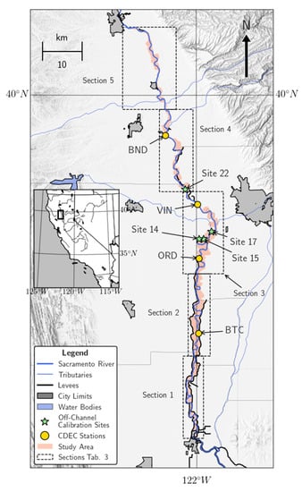
Figure 1.
Middle Sacramento River from Red Bluff to Colusa.
Two sets of remotely sensed imagery covering the area of interest were retrieved from Google Earth Engine catalog [47]: (1) Time-series of USGS LandSat-8 Surface Reflectance Tier 1 at 30 m resolution over the period 2014–2021 and (2) Time- series of Sentinel-2 MSI (MultiSpectral Instrument), Level-2A at 10–20 m resolution over the period 2018–2021. The band characteristics for both products are listed in Table 1. When several images were available for the same date covering different portions of the study area, they were combined and, if overlap existed, composited by selecting the highest-quality pixels, based on the absence of clouds and/or cloud shadows. On average, one image was available every 7–9 and 5–10 days, for LandSat-8 and Sentinel-2 products, respectively. Total number of images used in this effort and its distribution throughout the year is summarized in Table 2. Hydrologic data which observed daily Sacramento River flow (m3/s), were retrieved from the California Data Exchange Center (CDEC) for the stations at Hamilton City (HMC), Bend Bridge (BND), Vina Bridge (VIN), Ord-Ferry Channel (ORD), and Butte City (BTC) (Figure 1), for the period of available remotely sensed imagery. Levee spatial data were retrieved from the National Levee Database (https://levees.sec.usace.army.mil/; accessed on 1 June 2021).

Table 1.
Characteristics of USGS LandSat-8 and Sentinel-2 multispectral sensors.
Table 2.
Temporal distribution of number of used images from LandSat-8 and Sentinel-2 products.
2.2. Estimate of Inundation Extent
Inundation was extracted from multispectral imagery using the modified Normalized Difference Water Index (mNDWI) [57] and the Automated Water Extraction Index (AWEI) [58]. The first was based on NDWI proposed by McFeeters (1996), widely used in the first 10 years of the 21st century (e.g., [59,60]). [57] modification replaced the Near Infrared (NIR) band for the Short-wave Infrared (SWIR) band, since the latter can reflect subtle characteristics of water and is less sensitive to concentration of sediments and other constituents in the water than the NIR band [33], which expected during faster, more turbulent flows. This, in turn, makes mNDWI more stable and reliable than NDWI for floodplain delineation. The expression was developed based on a combination of reflectance in the green and shortwave-infrared (SWIR) wavelengths:
using bands 3 (Green), 6 (SWIR1) for LandSat-8 and 3, 11 for Sentinel-2 products, respectively (Table 1). The use of band ratios enhances the spectral signals by contrasting the reflectance between different wavelengths, reduces multiplicative noises (illumination differences, atmospheric attenuation, certain topographic variations), and allows comparison between different images through time and space [61,62].
The AWEI was developed to improve surface water identification from a time-series of LandSat-8 imagery, using a wider range of spectral bands, particularly from dark surfaces (e.g., shadows and built-up structures) with similar reflectance patterns [58]:
being bands 2 (Blue), 3 (Green), 5 (NIR), 6 (SWIR1), 7 (SWIR2) for LandSat-8, and 2 (Blue), 3 (Green), 8 (NIR), 11 (SWIR1), 12 (SWIR2) for Sentinel-2 products, respectively (Table 1). The equation coefficients were determined based on the analysis of the reflectance properties of different land cover types [58]. Due to the greater spectral response of water in the green and blue bands in respect to NIR and SWIR1 [63], water pixels should present large positive values. Then, NIR and SWIR2 bands help further differentiate water from other surfaces with similar reflectance characteristics by subtracting their value and forcing non-water pixels to present even larger negative values [58]. AWEIsh further improve the accuracy of AWEInsh to differentiate water pixels from shadow areas. Both indices were computed to determine the importance of shadow pixels in the area of interest.
Thresholding is a crucial issue in using water indices for delineating surface water areas. Generally, mNDWI values range from −1 to 1, with values over 0 representing surface water, based on its reflectance characteristics [33]. Likewise, AWEInsh over 0 indicate water features [58]. As such, a threshold of 0 is commonly used to identify surface water pixels [57,64]. Nevertheless, a slight calibration on the threshold value should be used to improve result accuracy [61], as shown by [33] and [34] that defined thresholds of −0.45 and 0.2 for mNDWI, and 0.25 for AWEInsh. Four surveyed off-channel habitats between Bend Bridge and Colusa (Table 3; Figure 1) were used to calibrate the threshold value for both indices by comparing computed values with periods of known inundation, identified from flow thresholds at Hamilton City station, reported by [18] and analyzing available images from expected inundation dates. The computed estimates were visually checked and corrected to avoid including misclassified cloud pixels in the analysis. Nevertheless, thresholding a time-series of images that cover the same water body is especially complicated as threshold index values might change for different overpass dates, and so may need to be fixed for each date independently [33,59]. Thus, the defined threshold from the site analysis was compared with an automatic water threshold recognition procedure, Otsu’s binarization algorithm, widely used with good results [33,65,66]. Google Earth Engine implementation of Otsu’s algorithm was provided by [67].
Table 3.
Off-channel water bodies used for mNDWI threshold calibration. Reference names and coordinates extracted from [17]. Location along the Sacramento River is shown in Figure 1.
Cloud and cloud shadow pixels were masked out of the composite images using algorithms developed by Google Earth Engine [47], based on LandSat-8 QA bands and Sentinel-2 cloud probability collection, before mNDWI and AWEI computation to avoid their misclassification as surface water areas. Images with cloud cover above 20% over the study area were removed from the time-series used for the analysis, as the cloud-free image would underestimate the existing inundated area. Likewise, Sacramento River mainstem pixels were extracted using the main channel area defined by the Central Valley Floodplain Evaluation and Delineation Program (CVFED) in their HEC-RAS/FLO-2D modeling efforts, to clearly differentiate off-channel areas. Furthermore, other OCWBs and water bodies disconnected to the Sacramento River within the study area were not considered in the inundated area calculations. Total off-channel habitat area for each available date was then computed by summing the area of pixels with indices’ values greater than the defined threshold. Image processing and computations were performed using the Google Earth Engine Python API.
Computed inundation extent was compared with surveyed values reported by [18] to determine if realistic magnitudes were obtained using the proposed method. Due to satellite overpass frequency, images during the peak of high-flow events were scarce, and those available exhibited cloud cover exceeding the 20% threshold. As such, off-channel area quantification mainly used remote imagery 2–5 days, on average, after the recorded flow peak. Nevertheless, it is assumed that they are representative of the expected off-channel extent for Sacramento River Pacific salmonids, as their rearing quality results from prolonged residence times to activate food production within the inundated areas [9]. Furthermore, the study area was divided into five sections, enumerated from south to north (Figure 1), covering the same latitude ranges (~0.18°) to study the distribution of off-channel areas along the mid-Sacramento River.
2.3. Off-Channel Habitat Availability
To inform conservation decisions for Pacific salmon along the mid-Sacramento River, suitable habitat must be identified from total off-channel inundation extent. The difference between off-channel inundation and available habitat extent resides on the combination of its physical characteristics and juvenile salmon bioenergetics [22,68]. As mainstem flows increase, the quality of already activated off-channel habitat might decline from optimal conditions (e.g., shallow, warmer water promoting zooplankton production and enhanced growth conditions [68,69,70]. As such, habitat type transitions from high-value off-channel habitat to poorer mainstem habitat [23]. This shift in growth potential is analogous to that reported from empirical experiments at Knaggs Ranch in Yolo Bypass (Katz, unpublished data), and detailed by [23]. Nevertheless, the described phenomenon does not imply that available off-channel habitat decreases with rising mainstem flows, as new shallow areas become active with greater stages. In turn, a “slow-down” in the rate of increasing habitat is expected after some flow threshold [71]. Remote sensing imagery is limited to the description of water inundation extent, requiring hydraulic modeling to determine water depths, velocities, and temperatures for a detailed representation of available off-channel habitat extent (e.g., [72]). As such, a rough approximation was developed by assuming threshold flows were reached at the minimum marginal increase in inundation extent, signaling an increase in river stage with little expansion in surface water area.
A flow-inundation area curve was fitted using 3rd order Chebyshev polynomials [73] to approximate the extent off-channel habitat at each mainstem flow state. All estimates of off-channel inundation computed in this study were used to fit the curve. The obtained flow-habitat curve has the following expression:
where ck are the fitted coefficients, Tk−1 is the Chebyshev polynomial of grade k − 1, A and B represent the upper and lower bound of the Sacramento River flows for which Equation (4) is valid (as Chebyshev polynomials are orthogonal), QSAC represents mainstem flow, and γ is a parameter representing the percentage of off-channel inundation that can be classified as suitable habitat for juvenile Pacific salmon, equal to 1 under threshold flows, and 0.25 otherwise.
2.4. Estimate of Off-Channel Habitat Residence Time
Water residence time within OCWB, after activation during high-flow events, largely determines the growth potential of Sacramento River Chinook salmon due to the required time for zooplankton development and consequent forage abundance [9] and higher water temperatures that boost juvenile growth [68,69,70]. As such, it is crucial to determine the time availability of OCWBs once they become activated to estimate their eventual impact on the development and population dynamics of Sacramento River salmonids. The change in inundated area within consecutive available images, during high-flow events with suitable cloud cover (<20%), was computed to determine the cut-off point when off-channel habitat was no longer available, at less than 0.4 km2 remaining, or when inundated areas became disconnected from the mainstem. This cut-off point represents the inundated extent under which fast dewatering was observed, a cue for juvenile Pacific salmon to leave these habitats to avoid stranding risks (similar to that observed in Yolo Bypass) [74].
3. Results
3.1. Indices’ Threshold
3.1.1. mNDWI
Computed mNDWI values at the four off-channel sites listed in Table 3 show a clear differentiation between dry and wet conditions for both LandSat-8 and Sentinel-2 products, especially at site 17, which required the highest flows to become active [18]. During dry conditions at the OCWBs, mainstem flows were well under activation thresholds (e.g., <200 m3/s), mNDWI values were consistently under −0.2, much less than the theoretical 0 threshold. Under wet conditions, when threshold flows were exceeded, values over −0.05 were extracted from the remote sensing image collection. Greater mNDWI values were obtained for increasing flows (Figure 2), from more prominent and deeper inundated areas, closer in spectral behavior to the mainstem (mNDWI > 0.4). Thus, the range from −0.2 to −0.06 was analyzed in more detail to establish an approximate threshold. Site 14 exhibited the most mNDWI values in this range, with several observations between −0.10 to −0.16 during May 2017 (LandSat-8) and June–August 2019 (LandSat-8 and Sentinel-2), when higher flows occurred (400–600 m3/s), but several weeks after high-flow storm events (>14 days). Additionally, several values were in the −0.2 to −0.15 range for low flows (<300 m3/s). An analysis of the images during these dates showed the site disconnected from the mainstem. As such, a final threshold for mNDWI of −0.08/−0.07, for LandSat-8 and Sentinel-2 products, respectively, was defined. Nevertheless, sites 14, 15, and 17 presented wetted conditions for flows under the required threshold (vertical dashed line in Figure 2). The analysis of the images represented by each data point (e.g., 17 March 2017 and 19 February 2019) showed that the off-channel areas were effectively inundated, from high flows occurring 4–11 days before the satellite overpass, and hence, were continuously activated during receding flows.
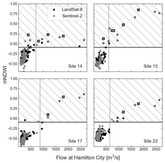
Figure 2.
Computed mNDWI values for surveyed off-channel habitats (Table 3) reported in [18] and existing daily Sacramento River flows recorded at Hamilton City (HMC). The hashed area indicates inundated conditions at the site. The vertical dashed line indicates required Sacramento River flows for off-channel activation [18]. Highlighted points represent dates when both single threshold and dynamic threshold identified the location as inundated.
The defined threshold was consistently lower than the automatic threshold values obtained with Otsu’s algorithm for all available images (Figure 3). This difference was especially important using LandSat-8 imagery, as computed thresholds were consistently positive (>0). Dynamic thresholds obtained from Sentinel-2 products were normally lower than those for LandSat-8 during overlapping dates, and closer to the defined single threshold. Data points recognized as inundated by both thresholding procedures were highlighted on Figure 2 and occurred on most dates with known wetted conditions (e.g., high flows during March 2019). Nevertheless, several inundated dates were only recognized using the single threshold at each location, with sites 14 and 22 having the highest proportion of misclassified conditions by the dynamic threshold (25–50% of inundated dates).
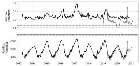
Figure 3.
Computed mNDWI and AWEIsh threshold values using Otsu’s binarization algorithm. Black line represents LandSat-8 products while gray line represents Sentinel-2 products. Dashed lines indicate defined single thresholds.
3.1.2. AWEInsh and AWEIsh
Computed AWEInsh at the analyzed sites presented a very erratic classification of inundated pixels, with significant differences in magnitude between sites (pairwise Mann–Whitney U test; p < 0.001). For instance, index values for known inundated dates at sites 15 and 22 were much lower than those representing dry conditions at site 14 (−2100 versus −1500). As such, a single threshold for all sites could not be defined, greatly reducing the expected accuracy of estimates using AWEInsh values. Thus, AWEInsh was not further considered and only AWEIsh was included in our analysis. A similar behavior than mNDWI values was computed for AWEIsh, considering its difference in magnitude, with certain dry conditions represented by values under −1500 (Figure 4). As for mNDWI, site 14 had the highest density of observations between this value and the theoretical threshold of 0. Detailed analysis of the −1500–0 range led to defining a threshold of AWEIsh = −310. Dynamic thresholding provided values much smaller than the defined threshold and even the considered land value (<−1500; Figure 3). As such, dynamic thresholding was not used to compute total inundated areas because of expected common misclassifications.
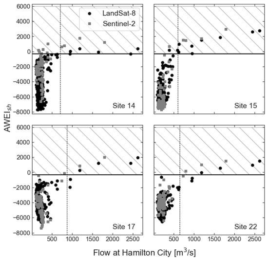
Figure 4.
Computed AWEI values for surveyed off-channel habitats (Table 3) reported in [18] and existing daily Sacramento River flows recorded at Hamilton City (HMC). The hashed area indicates inundated conditions at the site. The vertical dashed line indicates required Sacramento River flows for off-channel activation [18].
3.2. Mid-Sacramento River Inundated Area
3.2.1. Computed Inundated Area
Inundation extent estimates were computed using each available product (LandSat-8 and Sentinel-2), spectral index, and both single and dynamic threshold procedures. More detailed analysis on the effectiveness and accuracy of each procedure is presented in the following sections. A consequence of including each procedure is that quantified off-channel areas showed some dispersion, especially for low flows and small inundation areas (Figure 5).
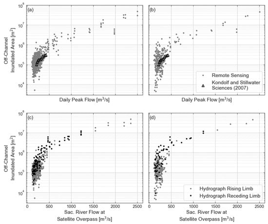
Figure 5.
Computed shallow areas extent along the mid-Sacramento River for each high-flow event peak using (a) mNDWI with single and dynamic thresholds and (b) AWEIsh single threshold. Surveyed estimates by [18] are also included for comparison. Subplots (c,d) show computed off-channel inundated areas against flows at satellite overpass for each water index.
Estimates agreed well with [18], whose values formed a lower bound of available off-channel areas along their reported flow range (Figure 5a,b), since they are only a subset of all OCWBs from Red Bluff to Colusa (those located on public land). Furthermore, they also show a similar increase rate in total wetted area per increase in mainstem flow, with a rapid increase between 200 to 350 m3/s (~40 m2/m3 s−1) followed by a slight decrease in expansion rate (~18 m2/m3 s−1) and, finally, significant gradual increases as flows exceed 700 m3/s (~240 m2/m3 s−1). Flows around 500 m3/s were needed to exceed 0.4 km2 of wetted surface consistently, but the subsequent rapid increase in inundated areas reached 4 km2 for flows ~1000 m3/s. Largest off-channel inundation extents (>20 km2) occurred during the greatest high-flow events on the available remote sensing imagery record (March 2017 and 2019), when flows along the Sacramento River mainstem exceeded 2000 m3/s.
OCWBs’ extent during the receding limb of the hydrograph were consistently higher than those from the rising limb for the same mainstem flows (~35%), visually identifiable when off-channel area estimates are plotted against Sacramento River daily flow at the date of satellite overpass (Figure 5c,d). They present a loop-like pattern, with two possible inundation extents depending on the timing of the image in respect to the high-flow event hydrograph. The difference is especially well-represented by the quantified off-channel areas for 1980 m3/s (4th highest peak flow in available images), which seemed to be underestimated when compared with the trend of the remaining high-flow data points (Figure 5a,b). However, source image was recorded 5 days after peak flows (14 February 2019 and 19 February 2019, respectively), during flow recession when mainstem flows were 472 m3/s (24% of the peak). Computed inundation was one order of magnitude greater than other events with mainstem flows of ~450 m3/s during the rising limb of the hydrograph (Figure 5c,d).
3.2.2. Flow-Inundation Relationship
Fitted flow-inundation area curve using Chebyshev polynomials (Figure 6) satisfactorily represented the complete mainstem flows range (fitted coefficients: ck = [5309.17, 8179.62, 3766.79, 1024.39]; RMSE = 1,271,690 m2; r2 = 0.86). Furthermore, it reasonably captured each described expansion rate region, i.e., fast increases in inundated area under 350 m3/s followed by a slowdown until around 700 m3/s and steady increases for higher flows. Minimum expansion rates of inundation area (13.6 m2/m3 s−1) occurred for flows of 648 m3/s, and hence, it was considered as threshold to differ further increases in inundation extent respect to off-channel habitat (parameter γ in Equation (5); Section 2.4).

Figure 6.
Fitted flow-habitat curve using Chebyshev polynomials and approximated suitable habitat.
3.2.3. Spatial Distribution of Inundated Areas
An uneven distribution of inundated areas was found along the mid-Sacramento River (Table 4). Most available intermitted wetted areas were located within Section 1, Section 2 and Section 3 for all the considered mainstem flow range, with more than 70% of the total area. This disproportion increased with higher flows, with the most upstream sections (4 and 5) accounting for less than 17% of the total. Section 3, around the confluence of Big Chico Creek, presented the greatest availability of off-channel areas for flows within 400–1000 m3/s, but not much greater than Section 1 and Section 2 (~20% more). Great expansions of inundated areas were not activated until peak flows exceeded 1000 m3/s along Section 1 (just north of Colusa), outweighing the remaining sections with more than double their wetted extents. This predominance persisted for flows over 1500 m3/s, but on a lesser extent (20–40% greater) as novel off-channel areas along Section 2 and Section 3 became activated under these flow conditions, especially within Section 2.
Table 4.
Average proportion (%) of total off-channel inundation extent under different mainstem flows along five Sacramento River sections (defined in Figure 1).
3.2.4. Estimates Comparison between Indices, Threshold Methodology, and Remote Sensing Products
mNDWI and AWEIsh indices led to similar estimates of off-channel inundation (r2 = 0.94; Figure 7f), especially for larger peak flows (areas over 1 km2). Nevertheless, mNDWI estimates seemed to slightly underestimate total inundation, in comparison, within that range (~7% lower). Larger divergences occurred at the opposite end of the range (areas under 0.4 km2), with mNDWI estimates being consistently bigger than those obtained with AWEIsh. For instance, mNDWI identified as inundated most of the side-channel pixels in Figure 8 (third location), while AWEIsh identified some of them as dry land, especially when LandSat-8 images were used.
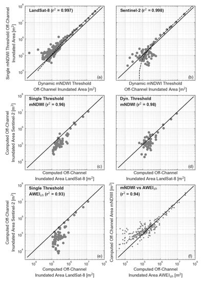
Figure 7.
Comparison of computed inundated areas using the different considered procedures: (a) dynamic mNDWI threshold versus single mNDWI threshold for LandSat-8; (b) Dynamic mNDWI threshold versus single mNDWI threshold using Sentinel-2; (c) mNDWI single threshold using LanSat-8 versus using Sentinel-2; (d) mNDWI dynamic threshold using LandSat-8 versus using Sentinel-2; (e) AWEIsh using LandSat-8 versus Sentinel-2, and (f) mNDWI (single and dynamic thresholds) vs. AWEIsh estimates using both LandSat-8 and Sentinel-2 products.

Figure 8.
Classified wetted pixels (blue areas) for the 16 March 2019 high-flow event at three specific locations along the mid-Sacramento River using the different indices, remote imagery products, and methodologies. Lighter blue represents shallower water areas.
Quantification of off-channel extent using a single threshold led to consistently greater estimates of inundated area than those defined with dynamic thresholds for both LandSat-8 and Sentinel-2 products (Figure 7a,b). Estimates for single threshold averaged 80% and 11% greater than for dynamic thresholds, with 5- and 3-fold maximum differences, for LandSat-8 and Sentinel-2, respectively. These larger percent differences between both procedures were for dates with low mainstem flows and minimal side-channel activation (e.g., 18 June 2016, 11 August 2018, 14 July 2019), for which any additional pixel classified as wet generated a big percent difference. The highest flow events on available remote imagery (March 2017, 2019) exhibited the largest differences in computed off-channel inundation with single threshold estimates over 4 km2 greater. This difference is shown by Figure 8, with greater extents of shallow-water habitat (lighter blue) identified using the single threshold, especially at the first location (first column). Nonetheless, defined inundation extents using both procedures presented a high correlation (r2 = 0.997 and 0.998; Figure 7a,b).
Computed total inundated area agreed well between LandSat-8 and Sentinel-2 products using mNDWI with dynamic thresholding (r2 = 0.98; Figure 7d). Inundated extents were consistently overestimated when computed with LandSat-8 imagery and using single thresholds for both indices, 36% and 323% greater on average for mNDWI and AWEIsh, respectively (Figure 7c,e). Biggest differences occurred for dates with smaller inundation extents across all indices and thresholding methods (Figure 7c–e). Nonetheless, for inundated areas under 1 km2, the difference between both estimates was under 0.12 and 0.2 km2 (on average) for mNDWI and AWEIsh, respectively.
3.3. Off-Channel Inundation Residence Time
Cloud coverage during several high-flow events available on the remote sensing record (e.g., February 2017) reduced the number of available storm events for this analysis. On average, shallow-water areas did not persist over 7–18 days, chiefly when storm events were isolated (e.g., Figure 9 and Figure 10). Nevertheless, during very wet periods (e.g., January–March 2017, 2019), when mainstem flows exceeded 1000 m3/s for extended periods, extensive off-channel inundation persisted for up to several months (>40 days).

Figure 9.
Off-channel inundated areas after 13 March 2016 storm event (hydrograph at bottom right corner) at two specific locations along the study area (black rectangle), extracted from LandSat-8 images using mNDWI with a single threshold (mNDWI > −0.08).

Figure 10.
Off-channel inundated areas after 8 April 2019 storm event (hydrograph at bottom right corner) at two specific locations along the study area (black rectangle), extracted from LandSat-8 images using mNDWI with a single threshold (mNDWI > −0.08). The green hydrograph represents flow conditions during 7 April 2018 high-flow event.
A detailed analysis of two events, March 2016 and April 2019 (Figure 8 and Figure 9, respectively), illustrates residence time computation. The regions for image comparison were selected based on differences in off-channel habitat type, with scour channels on point bars for the northern area (location of site 22) and side pools of various depths at the southern area. In 2016, satellite overpass occurred shortly after peak flows (1 day) showing almost the total inundation extent for the event, with the second overpass around 10 days later, similar to the first 2019 storm overpass (9 days). For both high-flow events, extensive off-channel inundation (blue areas) was still present after one week (~40% left in 2016). These generated images also showed a faster dewatering of scour channels for both events, but side pools presented a higher risk of stranding for juvenile salmon due to disconnection from the mainstem. Nonetheless, both events presented nearly dry conditions after 15–16 days after peak flows (Figure 9 and Figure 10). April 2018 and 2019 storm events had similar peak flows (1200–1400 m3/s) at almost identical dates (7th and 8th), but presented distinct receding limbs in their respective hydrographs (Figure 9). In 2018, the storm generated a narrow flood pulse with fast-receding flows (<5 days), while the 2019 storm exhibited more persistent decreasing flows (>10 days). Satellite overpass on 14 April 2018, only 7 days after the peak, registered almost non-existent shallow-water areas (<0.2 km2), while more extensive shallow-water areas were estimated for 24 April 2019 (1 km2), 16 days after peak flows.
4. Discussion
Off-channel habitats, particularly in highly modified rivers, are crucial to the development, survival, and long-term persistence of Sacramento River Pacific salmon (e.g., [21,22,23,75]). However, there is a paucity of information on quantitative descriptions of the existing extent and quality of shallow-water habitats, which can hinder their explicit consideration in proposed restoration or recovery actions, particularly for winter-run Chinook salmon [26,27,76]. Sparse efforts, mostly as part of larger spatial coverages, have reported general information such as off-channel area per river km or total extent (e.g., Pacific Rim) [28,45]. Nevertheless, these estimates, and the omission of the dynamic behavior of seasonal shallow habitat, which are key in their ecological value [9,21,22], might have generated little value to specific restoration efforts.
This study, building off the work of [18], developed a region-scale method to identify the extent and persistence of inundated OCWBs along the mid-Sacramento River. We show the potential of remote sensing imagery to quantify shallow-water areas and approximate average residence times (not previously found in literature), provide comparisons between different available remote sensing imagery (LandSat-8 and Sentinel-2) [47] and analysis procedures using spectral water indices (mNDWI and AWEIsh) [57,58]. These results have important implications for habitat restoration, as they could help managers and decision-makers develop recovery actions targeting juvenile salmon, such as defining flow pulses from reservoir releases and landform changes to expand shallow-water habitat. By incorporating this information and proposed restoration actions in juvenile production models (e.g., WRHAP-SEA) [23] and/or decision-making models (e.g., Winter-run DSM) [27], initial estimates of population response to proposed actions could also be generated.
4.1. Off-Channel Habitat Identification Using Spectral Indices, Threshold Methodology and Remote Sensing Products
Computed total inundated area agreed well between LandSat-8 and Sentinel-2 products for both water indices, similar to previously published analyses (e.g., [63,64]). As expected, the biggest differences occurred for dates with smaller inundation extents, when LandSat-8 estimates exceeded computed areas with Sentinel-2 images (Figure 7c–e). The higher resolution of Sentinel-2 products (20 m versus 30 m pixel size, Table 1), clearly identifiable in Figure 8 by more nitid images, allowed more precise identification of wet pixels under low-flow conditions, as partially wet LandSat-8 pixels might be classified as surface water despite a proportion of its surface being dry [66]. This is especially important for the defined single thresholds since their low values (<0) increase the chance of misidentifying partially wetted pixels as water. The first column of Figure 8 showed this tradeoff with a reduced extension of shallower areas (light blue) identified using Sentinel-2 versus LandSat-8. The lack of availability of Sentinel-2 products (end of 2018–present) greatly limited the range of mainstem high-flow events captured by the remote sensing imagery and did not allow for their exclusive use in this analysis.
mNDWI and AWEIsh single thresholds defined from image analysis of sites along the mid-Sacramento River were lower than the theoretical 0 value, but within the range used in literature [33,34,65,66]. The negative values were associated to the spectral characteristics of shallow-water areas, since their optical properties are not determined by water itself, but by other water components such as phytoplankton, suspended matter, and water depth [59,64,77]. This makes the spectral indices’ values closer to those of land rather than open water [34]. Both indices led to similar estimates of off-channel inundation (r2 = 0.94; Figure 7f), as reported in other areas [33,62,66,67]. Nonetheless, differences along the lower flow range suggested that AWEIsh classified inundated areas more accurately for the lowest flows. This was further supported by the bigger divergence between estimates from LandSat-8 and Sentinel-2 products (Figure 7e), due to improved classification combined with the higher resolution of Sentinel-2 images. These differences are easily spotted in the second location of Figure 8, when focusing on the identification of dry areas surrounded by inundation.
Otsu’s algorithm for automatic thresholding misclassified wet pixels with smaller inundation extents and/or shallower conditions, as shown in Figure 2 and Figure 4. This could be expected since the algorithm has been used to identify and delineate extensive surface water bodies (e.g., lakes, reservoirs) [65,66], whose optical characteristics differ from shallow waters [59,64,77]. As such, dynamic thresholding might underestimate the extent of activated side-channel features, especially during high peak flow events when defined thresholds were 0.05–0.2 (Figure 3) and transition areas of shallow water presented mNDWI values smaller than 0, misclassifying them as dry (Figure 7). These differences are shown in Figure 8, with identified shallow inundated areas (light blue) of lesser extent than using a single threshold at all locations. Likewise, the single threshold would be able to capture those transition areas, but it may also include other regions only partially or poorly connected (e.g., very shallow sections), and thus, overestimate available off-channel extent (Figure 8, first column). Nonetheless, defined inundation extents using both procedures presented a high correlation (r2 = 0.997 and 0.998 for LandSat-8 and Sentinel-2 products, respectively), suggesting that the proportion of misidentified pixels stayed consistent across images and mainstem flows. AWEIsh dynamic thresholds were not used in the analysis but several studies have shown a relatively stable optimal threshold (e.g., [33,58]), so accurate results could be achieved using a single threshold for the time-series of remote imagery [66].
4.2. Off-Channel Habitat Residence Time
The analysis of remote sensing imagery for recorded high-flow events allowed to discern the main drivers of off-channel inundation residence time. Wetted conditions at reported sites by [18] and total estimates of inundated areas showed continuous off-channel activation several days after the storm event (e.g., 4–11 days for Site 14 on 17 March 2017 and 19 February 2019), when mainstem receding flows were only a fraction of the peak. Furthermore, these inundation extents were consistently greater than the same flows during the onset of the storm event peak, showing an identifiable pattern on the distinct OCWBs’ behavior during rising and receding flows. The loop-like pattern (Figure 5c,d) results from flood wave propagation and unsteady flows along the Sacramento River, having for the same stage a higher discharge during rising flows than during the falling stage [78]. These effects generate distinctive loops in the stage–discharge relationship, referred to as hysteresis (e.g., [79,80]). Since river stage is the main driver of off-channel habitat activation, computed inundated area extent also showed this pattern. As such, inundation during receding flows showed greater extent for lower flow magnitudes, than rising limb wetted areas, due to the backwater effect of the flood wave [78].
The analysis of the storm events on 7 April 2018 and 8 April 2019 provided further insight into an important driver of residence time, associated with the hysteresis behavior described. In April 2019, residence times of 2 weeks were associated with high peak flows, and extensive initial inundation, and slow receding flows (>10 days). When compared to the storm event in April 2018, similar peak flows, and hence, initial inundation extents were computed. Nevertheless, the narrowness of the flood pulse with fast-receding flows (<5 days), led to marginal off-channel inundation (<0.2 km2) only 7 days after the peak. Therefore, residence time at off-channel areas depended mainly on the extent of the initial inundation and the flow rate of the decreasing limb, similar to other rivers systems (e.g., [81]).
4.3. Available Off-Channel Habitat
Computed estimates agreed well with values reported by [18], which formed a lower bound of available off-channel areas along their flow range (Figure 5a,b). This was expected since they represent only a subset of all OCWBs from Red Bluff to Colusa, which are those located on public land. Thus, moderate resolution of the remote sensing products employed (20 and 30 m; Table 1) allowed a satisfactory identification of reduced-sized off-channel habitat (such as scour channels) for higher-order rivers such as the Sacramento River, despite limitations in their coarse resolution to depict detailed shallow-water areas (e.g., [28]). A byproduct of considering each procedure, when combined with satellite band resolution, is that quantified off-channel areas show some dispersion, especially for low flows and small inundation areas (Figure 5). This was expected as pixels could be classified differently by each procedure, building proportional differences rapidly under low-flow conditions [33,61]. Nevertheless, since they represent situations with little off-channel availability (<0.4 km2), the dispersion does not pose critical differences on their potential for enhanced development of juvenile salmonids [23].
In addition to developing a dataset which describes expected off-channel inundation extent along the mid-Sacramento River for a range of mainstem flows, our objective was to quantify available off-channel habitat to inform conservation decisions for Pacific salmon. All estimates of off-channel inundation computed in this study were used to fit an off-channel habitat-flow curve, as each procedure and remote imagery product presented flow ranges with good and poor identification performances. For estimates obtained with a single threshold, the possible lack of stability of the threshold among image scenes was a problem [33,61], making it difficult to decide which value should be used in classification efforts for all image scenes. Our subjective choice of threshold (Section 3.1.1) based on surveyed OCWBs [18] might have affected the accuracy of the inundation estimates [58]. This was expected mainly during higher flow events, as the threshold’s negative value might have led to the misclassification of dry areas as shallow water. Similarly, Otsu’s algorithm dynamic thresholds seemed to misclassify wet pixels with a smaller inundation extent and/or shallower conditions (mNDWI ~ 0), and hence, dynamic thresholding might underestimate the total extent of inundated habitat. By combining all estimates, misclassification errors might be offset, allowing a more precise quantification of total off-channel habitat at different mainstem flows. This fitted relationship is an initial approximation of expected off-channel habitat along the mid-Sacramento River which allows for a primary analysis of their importance to Pacific salmon development and persistence (e.g., [23]). Nonetheless, it aims to motivate more detailed field surveys and hydraulic modeling at river sections of interest, developing a more robust inventory of off-channel habitat location, characteristics, and dynamic behavior.
4.4. Management Implications for Sacramento River Pacific Salmon
The management implications for the described dynamic behavior of off-channel areas and their quantification are extensive. Recently, there has been greater effort by resource managers to define environmental flow regimes to mimic ecologically relevant aspects of the annual natural hydrograph of regulated rivers, such as the Sacramento River (e.g., [82,83,84,85,86,87]). Such functional flow components sustain important ecosystem dynamics and have documented relationships with ecological, biogeochemical, and geomorphic processes in riverine systems [82]. An important framework that identifies and characterizes these hydrological features is the functional flows approach [87,88]. The framework recognizes over-bank flows as an important functional flow component (wet-season and fall pulse flows) [87,88,89] that supports a broad suite of physical and ecological processes, including the maintenance of habitat heterogeneity in space and time [90], providing cues for fish migration and entrainment in side-channel habitat [91], and controlling patterns of riparian succession [92]. As such, the fitted flow-habitat curve (Figure 6) and the relationship between off-channel activation period (i.e., residence time) and rate of receding flows are crucial to the design of optimal environmental pulse flows (i.e., magnitude, duration, and rate of change) to promote juvenile salmon use of shallow-water inundated areas, and hence, providing sufficient habitat with enhanced growth and survival conditions [22,23].
The quantification of shallow-water areas also showed little available habitat for flows under 400 m3/s (<0.75 km2), an important threshold anticipating juvenile winter-run Chinook peak migration across Knights Landing, downstream of Colusa [74]. This suggests that restoration actions should focus on enhancing horizontal connectivity between side-channel and mainstem habitats, and increasing off-channel habitat availability under lower flows (<400 m3/s). Such expansions would improve shallow-water areas for juvenile development prior to out-migration along the lower Sacramento River [23]. As commonly shared by CVPIA restoration practitioners, this defined restoration action targeting winter-run Chinook would also likely benefit other salmonids (Oncorhynchus spp.) or at a minimum, would not harm non-target salmonids [27].
Once desired restoration extents are drafted, the regional extent of remote sensing imagery allowed for the quantification of the spatial distribution of identified off-channel habitat for a range of mainstem flows (Table 4). This provides managers with regional information to focus such restoration actions. Section 1, Section 2 and Section 3 presented a disproportionally large amount of total activated off-channel habitat, with over 80% for greater flows. This has major implications and ramifications for migrating juvenile salmon, as limited refugia exists that might reduce migration survival across reaches downstream of Red Bluff, Section 4 and Section 5 (e.g., Brood Year 2008; Iglesias et al. 2017). These values suggest that expanding habitat along these sections might simultaneously address the lack of off-channel rearing habitat for winter-run Chinook (Table 4), and improve migration survival for other juvenile Pacific salmonids (e.g., fall-run Chinook, Central Valley steelhead). Similarly, the analysis showed the existence of extensive off-channel areas along Section 1 and Section 2 that require large peak flows (>1000 m3/s; Table 4) to become active. As such, restoration actions focused on improving the lateral connectivity of these areas might be able to rapidly increase available off-channel habitat for lower flows. Regardless, the combination of the reported estimates with more detailed studies on juvenile movement along mid-Sacramento River could help identify the river sections where an increase in habitat quality/extent would best improve Pacific salmon development and recovery.
5. Conclusions
This study showed the potential of moderate-resolution remote sensing imagery to characterize the spatiotemporal dynamics of off-channel habitat in higher-order rivers such as the Sacramento River. This method can cover a greater spatial extent than physical surveying, while simultaneously avoiding accessibility limitations on private lands. Obtained estimates with remote sensing were used to develop a database with which to analyze the distribution and temporal dynamics of off-channel areas along the mid-Sacramento River. The resulting database is not a substitute for physical surveying, but provides information for the design of effective flow pulses from reservoirs, and the regional assessment and prioritization of river reaches for Pacific Chinook salmon conservation. As such, it aims to motivate and bring focus on detailed field surveys and hydraulic modeling at identified river sections of interest, developing a more robust inventory of off-channel habitat location, characteristics, and dynamic behavior. For instance, limited habitat exists for flows under 400 m3/s, a cue for migration of endangered winter-run Chinook salmon, precluding juvenile access to areas with enhanced rearing conditions. Such restricted habitat is primarily in the upper reaches of the area of interest, limiting the available refugia of channel habitat during migration. Therefore, restoration actions focused on these reaches might provide greater ecological benefits. Our results aim to inform and influence conversations on needed off-channel habitat restoration using the presented rationale, and should be useful in refining conservation targets for Sacramento River Pacific Chinook salmon.
Author Contributions
Conceptualization, F.J.B.-L., R.A.L. and J.R.L.; Methodology, F.J.B.-L.; Data Curation, F.J.B.-L.; Formal Analysis, F.J.B.-L.; Visualization, F.J.B.-L.; Resources, R.A.L. and J.R.L.; Funding Acquisition, J.R.L.; Supervision, R.A.L. and J.R.L.; Writing-Original Draft, F.J.B.-L.; Writing—Review and Editing, F.J.B.-L., R.A.L. and J.R.L. All authors have read and agreed to the published version of the manuscript.
Funding
Financial support of this research came from U.S. Department of Energy (DOE Prime Award No. DE-IA0000018).
Data Availability Statement
LandSat-8 and Sentinel-2 products were accessed through the Google Earth Engine platform.
Acknowledgments
We thank Eric Holmes for providing valuable input on the potential of remote sensing imagery to map habitat. This paper also benefited from thoughtful comments from two anonymous reviewers.
Conflicts of Interest
The authors declare no conflict of interest.
References
- Kondolf, G.M.; Montgomery, D.R.; Piégay, H.; Schmitt, L. Geomorphic classification of rivers and streams. Tools Fluv. Geomorphol. 2003, 7, 171–204. [Google Scholar]
- Lewin, J.; Brewer, P.A.; Wohl, E. Fluvial Geomorphology. In Reference Module in Earth Systems and Environmental Sciences; Elsevier: Amsterdam, The Netherlands, 2018. [Google Scholar]
- Junk, W.J.; Bayley, P.B.; Sparks, R.E. The flood pulse concept in river-floodplain systems. Can. Spec. Publ. Fish. Aquat. Sci. 1989, 1061, 110–127. [Google Scholar]
- Sommer, T.R.; Nobriga, M.L.; Harrell, W.C.; Batham, W.; Kimmerer, W.J. Floodplain rearing of juvenile Chinook salmon: Evidence of enhanced growth and survival. Can. J. Fish. Aquat. Sci. 2001, 58, 325–333. [Google Scholar] [CrossRef]
- Tockner, K.; Stanford, J.A. Riverine flood plains: Present state and future trends. Environ. Conserv. 2002, 29, 308–330. [Google Scholar] [CrossRef] [Green Version]
- Opperman, J.J.; Luster, R.; McKenney, B.A.; Roberts, M.; Meadows, A.W. Ecologically Functional Floodplains: Connectivity, Flow Regime, and Scale1. JAWRA J. Am. Water Resour. Assoc. 2010, 46, 211–226. [Google Scholar] [CrossRef]
- Grosholz, E.; Gallo, E. The influence of flood cycle and fish predation on invertebrate production on a restored California floodplain. Hydrobiologia 2006, 568, 91–109. [Google Scholar] [CrossRef]
- Ahearn, D.S.; Viers, J.H.; Mount, J.F.; Dahlgren, R.A. Priming the productivity pump: Flood pulse driven trends in suspended algal biomass distribution across a restored floodplain. Freshw. Biol. 2006, 51, 1417–1433. [Google Scholar] [CrossRef]
- Corline, N.J.; Sommer, T.; Jeffres, C.A.; Katz, J. Zooplankton ecology and trophic resources for rearing native fish on an agricultural floodplain in the Yolo Bypass California, USA. Wetl. Ecol. Manag. 2017, 25, 533–545. [Google Scholar] [CrossRef]
- Humphries, P.; King, A.J.; Koehn, J.D. Fish, Flows and Flood Plains: Links between Freshwater Fishes and their Environment in the Murray-Darling River System, Australia. J. Appl. Phycol. 1999, 56, 129–151. [Google Scholar] [CrossRef]
- Lytle, D.A.; Poff, N.L. Adaptation to natural flow regimes. Trends Ecol. Evol. 2004, 19, 94–100. [Google Scholar] [CrossRef]
- Whited, D.C.; Kimball, J.S.; Lucotch, J.A.; Maumenee, N.K.; Wu, H.; Chilcote, S.D.; Stanford, J.A. A Riverscape Analysis Tool Developed to Assist Wild Salmon Conservation Across the North Pacific Rim. Fisheries 2012, 37, 305–314. [Google Scholar] [CrossRef]
- Gallart, F.; Llorens, P.; Latron, J.; Cid, N.; Rieradevall, M.; Prat, N. Validating alternative methodologies to estimate the regime of temporary rivers when flow data are unavailable. Sci. Total Environ. 2016, 565, 1001–1010. [Google Scholar] [CrossRef] [PubMed]
- Roni, P.; Hall, J.E.; Drenner, S.M.; Arterburn, D. Monitoring the effectiveness of floodplain habitat restoration: A review of methods and recommendations for future monitoring. WIREs Water 2019, 6, 1355. [Google Scholar] [CrossRef]
- Sommer, T.R.; Harrell, W.C.; Solger, A.M.; Tom, B.; Kimmerer, W. Effects of flow variation on channel and floodplain biota and habitats of the Sacramento River, California, USA. Aquat. Conserv. Mar. Freshw. Ecosyst. 2004, 14, 247–261. [Google Scholar] [CrossRef]
- Kelley, R. Battling the Inland Sea: Floods, Public Policy, and the Sacramento Valley; University of California Press: Berkeley, CA, USA, 1989. [Google Scholar]
- Hanak, E.; Lund, J.R.; Dinar, A.; Gray, B.; Howitt, R.; Mount, J.; Moyle, P.; Thompson, B. Managing California’s Water: From Conflict to Reconciliation; Public Policy Institute of California: San Francisco, CA, USA, 2011. [Google Scholar]
- Kondolf, G.M.; Stillwater Sciences. Sacramento River Ecological Flows Study: Off-Channel Habitat Study Results; Technical Report prepared for The Nature Conservancy; Kondolf, G.M., Ed.; Stillwater Sciences: Berkeley, CA, USA; Chico, CA, USA, 2007. [Google Scholar]
- Moyle, P.B. Inland Fishes of California: Revised and Expanded; University of California Press: Berkeley, CA, USA, 2002. [Google Scholar]
- U.S. Bureau of Reclamation (USBR). Reinitiation of Consultation on the Coordinated Long-Term Operation of the Central Vallley Project and State Water Project. Final Biological Assessment; U.S. Department of the Interior: Washington, DC, USA, 2019.
- Maslin, P.E.; McKinney, W.R.; Moore, T.L. Intermittent streams as rearing habitat for Sacramento River Chinook salmon. In Anadromous Fish Restoration Program; United States Fish and Wildlife Service, Stockton: Washington, DC, USA, 1996. [Google Scholar]
- Limm, M.P.; Marchetti, M.P. Juvenile Chinook salmon (Oncorhynchus tshawytscha) growth in off-channel and main-channel habitats on the Sacramento River, CA using otolith increment widths. J. Appl. Phycol. 2009, 85, 141–151. [Google Scholar] [CrossRef] [Green Version]
- Bellido-Leiva, F.J.; Lusardi, R.A.; Lund, J.R. Modeling the effect of habitat availability and quality on endangered winter-run Chinook salmon (Oncorhynchus tshawystscha) production in the Sacramento Valley. Ecol. Model. 2021, 447, 109511. [Google Scholar] [CrossRef]
- Woodson, L.E.; Wells, B.K.; Weber, P.K.; MacFarlane, R.B.; Whitman, G.E.; Johnson, R.C. Size, growth, and origin-dependent mortality of juvenile Chinook salmon Oncorhynchus tshawytscha during early ocean residence. Mar. Ecol. Prog. Ser. 2013, 487, 163–175. [Google Scholar] [CrossRef] [Green Version]
- Yoshiyama, R.M.; Fisher, F.W.; Moyle, P.B. Historical Abundance and Decline of Chinook Salmon in the Central Valley Region of California. N. Am. J. Fish. Manag. 1998, 18, 487–521. [Google Scholar] [CrossRef]
- National Marine Fisheries Service (NMFS). Recovery Plan for the Evolutionarily Significant Units of Sacramento River Winter-Run Chinook Salmon and Central Valley Spring-Run Chinook Salmon and the Distinct Population Segment of California Central Valley Steelhead; California Central Valley Area Office: Sacramento, CA, USA, 2014.
- Peterson, J.T.; Duarte, A. Decision analysis for greater insights into the development and evaluation of Chinook salmon restoration strategies in California’s Central Valley. Restor. Ecol. 2020, 28, 1596–1609. [Google Scholar] [CrossRef]
- Whited, D.C.; Kimball, J.S.; Lorang, M.S.; Stanford, J.A. Estimation of juvenile salmon habitat in Pacific Rim rivers using multiscalar remote sensing and geospatial analysis. River Res. Appl. 2013, 29, 135–148. [Google Scholar] [CrossRef]
- Chen, Y.; Cuddy, S.M.; Wang, B.; Merrin, L.E.; Pollock, D.; Sims, N. Linking inundation timing and extent to ecological response models using the Murray-Darling Basin Floodplain Inundation Model (MDB-FIM). In Proceedings of the MODSIM2011, 19th International Congress on Modelling and Simulation, Perth, Australia, 12–15 December 2011; Chan, F., Marinova, D., Anderssen, R.S., Eds.; Modelling and Simulation Society of Australia and New Zealand: Perth, Australia, 2011; pp. 4092–4098. [Google Scholar]
- Huang, C.; Chen, Y.; Wu, J.; Yu, J. Detecting floodplain inundation frequency using MODIS time-series imagery. In Proceedings of the 1st International Conference on Agro-Geoinformatics (Agro-Geoinformatics2012), Shanghai, China, 2–4 August 2012. [Google Scholar]
- Huang, C.; Chen, Y.; Wu, J. A DEM-based modified pixel swapping algorithm for floodplain inundation mapping at subpixel scale. In Proceedings of the 2013 IEEE International Geoscience and Remote Sensing Symposium (IGASS), Melbourne, Australia, 21–26 July 2013. [Google Scholar]
- Huang, C.; Chen, Y.; Wu, J. Mapping spatio-temporal flood inundation dynamics at large river basin scale using time-series flow data and MODIS imagery. Int. J. Appl. Earth Obs. Geoinf. 2014, 26, 350–362. [Google Scholar] [CrossRef]
- Huang, C.; Chen, Y.; Zhang, S.; Wu, J. Detecting, Extracting, and Monitoring Surface Water From Space Using Optical Sensors: A Review. Rev. Geophys. 2018, 56, 333–360. [Google Scholar] [CrossRef]
- Chen, Y.; Wang, B.; Pollino, C.; Cuddy, S.; Merrin, L.; Huang, C. Estimate of flood inundation and retention on wetlands using remote sensing and GIS. Ecohydrology 2013, 7, 1412–1420. [Google Scholar] [CrossRef]
- Wang, Y.; Colby, J.D.; Mulcahy, K.A. An efficient method for mapping flood extent in a coastal flood plain using Landsat TM and DEM data. Int. J. Remote Sens. 2002, 23, 3681–3696. [Google Scholar] [CrossRef]
- Frazier, P.; Page, K.; Louis, J.; Briggs, S.; Robertson, A. Relating wetland inundation to river flow using Landsat TM data. Int. J. Remote Sens. 2003, 24, 3755–3770. [Google Scholar] [CrossRef]
- Knebl, M.R.; Yang, Z.L.; Hutchison, K.; Maidment, D.R. Regional scale flood modelling using NEXRAD, rainfall, GIS and HEC-HMS\RAS: A case study for the San Antonio River basin summer 2002 storm event. J. Environ. Manag. 2005, 75, 325–336. [Google Scholar] [CrossRef] [PubMed]
- Gupta, A.; Liew, S.C. The Mekong from satellite imagery: A quick look at a large river. Geomorphology 2007, 85, 259–274. [Google Scholar] [CrossRef]
- Hou, J.; van Dijk, A.I.J.M.; Renzullo, L.J.; Vertessy, R.A.; Mueller, N. Hydromorphological attributes for all Australian river reaches derived from Landsat dynamic inundation remote sensing. Earth Syst. Sci. Data 2019, 11, 1003–1015. [Google Scholar] [CrossRef] [Green Version]
- Brennan, S.R.; Schindler, D.E.; Cline, T.J.; Walsworth, T.E.; Buck, G.; Fernandez, D.P. Shifting habitat mosaics and fish production across river basins. Science 2019, 364, 783–786. [Google Scholar] [CrossRef] [PubMed]
- Whited, D.C.; Stanford, J.A.; Kimball, J.S. Application of airborne multispectral digital imagery to characterize riverine habitats at different base flows. River Res. Appl. 2002, 18, 583–594. [Google Scholar] [CrossRef]
- Gilvear, D.J.; Davids, C.; Tyler, A.N. The use of remotely sensed data to detect channel hydromorphology; River Tummel, Scotland. River Res. Appl. 2004, 20, 795–811. [Google Scholar] [CrossRef]
- Gilvear, D.J.; Sutherland, P.; Higgins, T. An assessment of the use of remote sensing to map habitat features important to sustaining lamprey populations. Aquat. Conserv. Mar. Freshw. Ecosyst. 2008, 18, 807–818. [Google Scholar] [CrossRef]
- Legleiter, C.J.; Roberts, D.A.; Marcus, W.A.; Fonstad, M.A. Passive optical remote sensing of river channel morphology and in-stream habitat: Physical basis and feasibility. Remote Sens. Environ. 2004, 93, 493–510. [Google Scholar] [CrossRef] [Green Version]
- Luck, M.A.; Maumenee, N.; Whited, D.; Lucotch, J.; Chilcote, S.; Lorang, M.; Goodman, D.; McDonald, K.; Kimball, J.; Stanford, J. Remote sensing analysis of physical complexity of North Pacific Rim rivers to assist wild salmon conservation. Earth Surf. Processes Landf. 2010, 35, 1330–1342. [Google Scholar] [CrossRef]
- Wirth, L.; Rosenberger, A.; Prakash, A.; Gens, R.; Margraf, F.J.; Hamazaki, T. A Remote-Sensing, GIS-Based Approach to Identify, Characterize, and Model Spawning Habitat for Fall-Run Chum Salmon in a Sub-Arctic, Glacially Fed River. Trans. Am. Fish. Soc. 2012, 141, 1349–1363. [Google Scholar] [CrossRef]
- Gorelick, N.; Hancher, M.; Dixon, M.; Ilyushchenko, S.; Thau, D.; Moore, R. Google Earth Engine: Planetary-scale geospatial analysis for everyone. Remote Sens. Environ. 2017, 202, 18–27. [Google Scholar] [CrossRef]
- Ward, J.V.; Tockner, K.; Arscott, D.B.; Claret, C. Riverine landscape diversity. Freshw. Biol. 2002, 47, 517–539. [Google Scholar] [CrossRef] [Green Version]
- Whited, D.C.; Lorang, M.S.; Harner, M.J.; Hauer, F.R.; Kimball, J.S.; Stanford, J.A. Climate, Hydrologic Disturbance, and Succession: Drivers of Floodplain Pattern. Ecology 2007, 88, 940–953. [Google Scholar] [CrossRef] [Green Version]
- Stanford, J.A.; Lorang, M.S.; Hauer, F.R. The shifting habitat mosaic of river ecosystems. Int. Ver. Theor. Angew. Limnol. 2005, 29, 123–136. [Google Scholar] [CrossRef]
- Shelton, M.L. Unimpaired and Regulated Discharge in the Sacramento River Basin, California. Yearb. Assoc. Pac. Coast Geogr. 1995, 57, 134–157. [Google Scholar] [CrossRef]
- Ralph, F.M.; Cordeira, J.M.; Neiman, P.J.; Hughes, M. Landfalling Atmospheric Rivers, the Sierra Barrier Jet, and Extreme Daily Precipitation in Northern California’s Upper Sacramento River Watershed. J. Hydrometeorol. 2016, 17, 1905–1914. [Google Scholar] [CrossRef]
- Kim, J.; Waliser, D.E.; Neiman, P.J.; Guan, B.; Ryoo, J.-M.; Wick, G.A. Effects of atmospheric river landfalls on the cold season precipitation in California. Clim. Dyn. 2013, 40, 465–474. [Google Scholar] [CrossRef]
- Kingsmill, D.E.; Neiman, P.J.; Moore, B.J.; Hughes, M.; Yuter, S.E.; Ralph, F.M. Kinematic and Thermodynamic Structures of Sierra Barrier Jets and Overrunning Atmospheric Rivers during a Landfalling Winter Storm in Northern California. Mon. Weather Rev. 2013, 141, 2015–2036. [Google Scholar] [CrossRef] [Green Version]
- Wohl, E.; Lane, S.N.; Wilcox, A.C. The science and practice of river restoration. Water Resour. Res. 2015, 51, 5974–5997. [Google Scholar] [CrossRef] [Green Version]
- Sommer, T.R.; Baxter, R.D.; Feyrer, F. Splittail Delisting: A Review of Recent Population Trends and Restoration Activities. Am. Fish. Soc. Symp. 2007, 53, 38. [Google Scholar]
- Xu, H. Modification of normalised difference water index (NDWI) to enhance open water features in remotely sensed imagery. Int. J. Remote Sens. 2006, 27, 3025–3033. [Google Scholar] [CrossRef]
- Feyisa, G.L.; Meilby, H.; Fensholt, R.; Proud, S.R. Automated Water Extraction Index: A new technique for surface water mapping using Landsat imagery. Remote Sens. Environ. 2014, 140, 23–35. [Google Scholar] [CrossRef]
- Chowdary, V.; Chandran, R.V.; Neeti, N.; Bothale, R.; Srivastava, Y.; Ingle, P.; Ramakrishnan, D.; Dutta, D.; Jeyaram, A.; Sharma, J.; et al. Assessment of surface and sub-surface waterlogged areas in irrigation command areas of Bihar state using remote sensing and GIS. Agric. Water Manag. 2008, 95, 754–766. [Google Scholar] [CrossRef]
- Hui, F.; Xu, B.; Huang, H.; Yu, Q.; Gong, P. Modelling spatial-temporal change of Poyang Lake using multitemporal Landsat imagery. Int. J. Remote Sens. 2008, 29, 5767–5784. [Google Scholar] [CrossRef]
- Ji, L.; Zhang, L.; Wylie, B. Analysis of dynamic thresholds for the normalized difference water index. Photogramm. Eng. Remote Sens. 2009, 75, 1307–1317. [Google Scholar] [CrossRef]
- Mohammadi, A.; Costelloe, J.F.; Ryu, D. Application of time series of remotely sensed normalized difference water, vegetation and moisture indices in characterizing flood dynamics of large-scale arid zone floodplains. Remote Sens. Environ. 2017, 190, 70–82. [Google Scholar] [CrossRef]
- Mishra, V.K.; Pant, T. Open surface water index: A novel approach for surface water mapping and extraction using multispectral and multisensory data. Remote Sens. Lett. 2020, 11, 973–9822. [Google Scholar] [CrossRef]
- Zhou, Y.; Dong, J.; Xiao, X.; Xiao, T.; Yang, Z.; Zhao, G.; Zhenhua, Z.; Qin, Y. Open surface water mapping algorithms: A comparison of water-related spectral indices and sensors. Water 2017, 9, 256. [Google Scholar] [CrossRef]
- Du, Z.; Li, W.; Zhou, D.; Tian, L.; Ling, F.; Wang, H.; Gui, Y.; Sun, B. Analysis of Landsat-8 OLI imagery for land surface water mapping. Remote Sens. Lett. 2014, 5, 672–681. [Google Scholar] [CrossRef]
- Xie, H.; Luo, X.; Xu, X.; Pan, H.; Tong, X. Evaluation of Landsat 8 OLI imagery for unsupervised inland water extraction. Int. J. Remote Sens. 2016, 37, 1826–1844. [Google Scholar] [CrossRef]
- Li, J.; Peng, B.; Wei, Y.; Ye, H. Accurate extraction of surface water in complex environment based on Google Earth Engine and Sentinel-2. PLoS ONE 2021, 16, e0253209. [Google Scholar] [CrossRef] [PubMed]
- Lusardi, R.A.; Hammock, B.G.; Jeffres, C.A.; Dahlgren, R.; Kiernan, J.D. Oversummer growth and survival of juvenile coho salmon (Oncorhynchus kisutch) across a natural gradient of stream water temperature and prey availability: An in situ enclosure experiment. Can. J. Fish. Aquat. Sci. 2020, 77, 413–424. [Google Scholar] [CrossRef]
- Jeffres, C.A.; Holmes, E.J.; Sommer, T.R.; Katz, J.V. Detrital food web contributes to aquatic ecosystem productivity and rapid salmon growth in a managed floodplain. PLoS ONE 2020, 15, e0216019. [Google Scholar] [CrossRef]
- Zillig, K.W.; Lusardi, R.A.; Moyle, P.B.; Fangue, N.A. One size does not fit all: Variation in thermal eco-physiology among Pacific salmonids. Rev. Fish Biol. Fish. 2021, 31, 95–114. [Google Scholar] [CrossRef]
- Lyon, J.; Stuart, I.; Ramsey, D.; O’Mahony, J. The effect of water level on lateral movements of fish between river and off-channel habitats and implications for management. Mar. Freshw. Res. 2010, 61, 271–278. [Google Scholar] [CrossRef] [Green Version]
- Lacey, R.W.; Millar, R.G. Reach scale hydraulic assessment of instream salmonid habitat restoration. JAWRA J. Am. Water Resour. Assoc. 2004, 40, 1631–1644. [Google Scholar] [CrossRef]
- Mason, J.C.; Handscomb, D.C. Chebyshev Polynomials; CRC Press: Boca Raton, FL, USA, 2002. [Google Scholar]
- del Rosario, R.B.; Redler, Y.J.; Newman, K.; Brandes, P.L.; Sommer, T.; Reece, K.; Vincik, R. Migration Patterns of Juvenile Winter-run-sized Chinook Salmon (Oncorhynchus tshawytscha) through the Sacramento–San Joaquin Delta. San Fr. Estuary Watershed Sci. 2013, 11, 1–22. [Google Scholar] [CrossRef] [Green Version]
- Moyle, P.B.; Lusardi, R.A.; Samuel, P.J.; Katz, J.V. State of the Salmonids: Status of California’s Emblematic Fishes, 2017; Technical Report prepared for California Trout; University of California: Davis, CA, USA, 2017. [Google Scholar]
- National Marine Fisheries Service (NMFS). Species in the Spotlight: Sacramento River Winter-run Chinook Salmon. Priority Actions 2021–2025; California Central Valley Area Office: Sacramento, CA, USA, 2021.
- Yagmur, N.; Musaoglu, N.; Taskin, G. Detection of Shallow Water area with Machine Learning Algorithms. ISPRS Int. Arch. Photogramm. Remote Sens. Spat. Inf. Sci. 2019, XLII-2/W13, 1269–1273. [Google Scholar] [CrossRef] [Green Version]
- Petersen-Øverleir, A. Modelling stage—discharge relationships affected by hysteresis using the Jones formula and nonlinear regression. Hydrol. Sci. J. 2006, 51, 365–388. [Google Scholar] [CrossRef] [Green Version]
- Chow, V.T. Open-Channel Hydraulics; McGraw-Hill: New York, NY, USA, 1959. [Google Scholar]
- Fenton, J.D.; Keller, R.J. The Calculation of Streamflow from Measurements of Stage; Report 01/6; CRC for Catchment Hydrology: Victoria, Australia, September 2001; p. 84. [Google Scholar]
- Czuba, J.A.; David, S.R.; Edmonds, D.A.; Ward, A.S. Dynamics of surface-water connectivity in a low-gradient meandering river floodplain. Water Resour. Res. 2019, 55, 1849–1870. [Google Scholar] [CrossRef]
- Yarnell, S.M.; Petts, G.E.; Schmidt, J.C.; Whipple, A.A.; Beller, E.E.; Dahm, C.N.; Goodwin, P.; Viers, J.H. Functional Flows in Modified Riverscapes: Hydrographs, Habitats and Opportunities. Bioscience 2015, 65, 963–972. [Google Scholar] [CrossRef] [Green Version]
- Horne, A.; Szemis, J.M.; Kaur, S.; Webb, J.A.; Stewardson, M.J.; Costa, A.; Boland, N. Optimization tools for environmental water decisions: A review of strengths, weaknesses, and opportunities to improve adoption. Environ. Modell. Softw. 2016, 84, 326–338. [Google Scholar] [CrossRef]
- Horne, A.; Kaur, S.; Szemis, J.; Costa, A.; Webb, J.A.; Nathan, R.; Stewardson, M.; Lowe, L.; Boland, N. Using optimization to develop a “designer” environmental flow regime. Environ. Model. Softw. 2017, 88, 188–199. [Google Scholar] [CrossRef]
- Chen, W.; Olden, J.D. Designing flows to resolve human and environmental water needs in a dam-regulated river. Nat. Commun. 2017, 8, 2158. [Google Scholar] [CrossRef] [PubMed]
- Lane, B.; Ortiz-Partida, J.P.; Sandoval-Solis, S. Extending water resources performance metrics to river ecosystems. Ecol. Indic. 2020, 114, 106336. [Google Scholar] [CrossRef] [Green Version]
- Stein, E.D.; Zimmerman, J.; Yarnell, S.M.; Stanford, B.; Lane, B.; Taniguchi-Quan, K.T.; Obester, A.; Grantham, T.E.; Lusardi, R.A.; Sandoval-Solis, S. The California Environmental Flows Framework: Meeting the Challenges of Developing a Large-Scale Environmental Flows Program. Front. Environ. Sci. 2021, 9, 481. [Google Scholar] [CrossRef]
- Yarnell, S.M.; Stein, E.D.; Webb, J.A.; Grantham, T.; Lusardi, R.A.; Zimmerman, J.; Peek, R.A.; Lane, B.A.; Howard, J.; Sandoval-Solis, S. A functional flows approach to selecting ecologically relevant flow metrics for environmental flow applications. River Res. Appl. 2020, 36, 318–324. [Google Scholar] [CrossRef]
- Palmer, M.; Ruhi, A. Linkages between flow regime, biota, and ecosystem processes: Implications for river restoration. Science 2019, 365, eaaw2087. [Google Scholar] [CrossRef] [PubMed] [Green Version]
- Ward, J. Riverine landscapes: Biodiversity patterns, disturbance regimes, and aquatic conservation. Biol. Conserv. 1998, 83, 269–278. [Google Scholar] [CrossRef]
- Jeffres, C.A.; Opperman, J.J.; Moyle, P.B. Ephemeral floodplain habitats provide best growth conditions for juvenile Chinook salmon in a California river. J. Appl. Phycol. 2008, 83, 449–458. [Google Scholar] [CrossRef]
- Ward, J.V.; Stanford, J.A. Ecological connectivity in alluvial river ecosystems and its disruption by flow regulation. Regul. Rivers Res. Manag. 1995, 11, 105–119. [Google Scholar] [CrossRef]
Publisher’s Note: MDPI stays neutral with regard to jurisdictional claims in published maps and institutional affiliations. |
© 2022 by the authors. Licensee MDPI, Basel, Switzerland. This article is an open access article distributed under the terms and conditions of the Creative Commons Attribution (CC BY) license (https://creativecommons.org/licenses/by/4.0/).