Cloud-Based Monitoring and Evaluation of the Spatial-Temporal Distribution of Southeast Asia’s Mangroves Using Deep Learning

Abstract

This paper proposes a cloud-based mangrove monitoring framework that uses Google Collaboratory and Google Earth Engine to classify mangroves in Southeast Asia (SEA) using satellite remote sensing imagery (SRSI). Three multi-class classification convolutional neural network (CNN) models were generated, showing F1-score values as high as 0.9 in only six epochs of training. Mangrove forests are tropical and subtropical environments that provide essential ecosystem services to local biota and coastal communities and are considered the most efficient vegetative carbon stock globally. Despite their importance, mangrove forest cover continues to decline worldwide, especially in SEA. Scientists have produced monitoring tools based on SRSI and CNNs to identify deforestation hotspots and drive targeted interventions. Nevertheless, although CNNs excel in distinguishing between different landcover types, their greatest limitation remains the need for significant computing power to operate. This may not always be feasible, especially in developing countries. The proposed framework is believed to provide a robust, low-cost, cloud-based, near-real-time monitoring tool that could serve governments, environmental agencies, and researchers, to help map mangroves in SEA.

1. Introduction

Mangrove forests are unique tropical and subtropical ecosystems located at the intersections between land and coastal environments [1]. Mangrove trees have the unique ability to live in saline ecosystems because they have evolved to use salt in their photosynthesis and struggle to grow in its absence [2]. Due to their locations, mangroves provide numerous essential ecosystem services to coastal communities [3]. They sustain marine and terrestrial habitats [4], mitigate the impacts of tsunamis and storms on coastlines [5], support local fisheries [6], and efficiently sequester carbon [7]. Nonetheless, although mangroves play an essential role within their habitats [1,8], their cover has been declining globally for the past two decades due to deforestation, with the most extensive removal occurring in Southeast Asia (SEA) [9], where exploitative illegal activities [10] and the growth of agriculture and aquaculture as parts of aggressive economic strategies [1,10] are key drivers of mangrove loss [5].

Although mangrove forests only make up 0.7% of the global tropical forest cover [8], they account for ~50% of the global carbon stock worldwide [7], sequestering around four times the amount of carbon of inland tropical forests [1]. Scientists estimate that mangrove deforestation alone is responsible for ~10% of the global annual carbon released into the atmosphere [8]. The figure is particularly relevant for SEA, which alone accounts for ~30% of the global mangrove forest cover [11]. Thus, the aggressive removal of mangroves in SEA disrupts local ecosystems and has global implications, particularly on global net carbon frameworks and climate change mitigation efforts [12,13].

Mangrove forests are long strips of trees along coasts and rivers [11], and studies have often failed to distinguish them from other inland forests using satellite remote sensing imagery (SRSI) [1,10]. Although the scientific community has endeavoured to produce highly accurate maps using ever-advancing remote sensing technologies [14], mapping mangroves remains challenging [15]. In a study on global mangrove distribution mapping by Bunting et al. 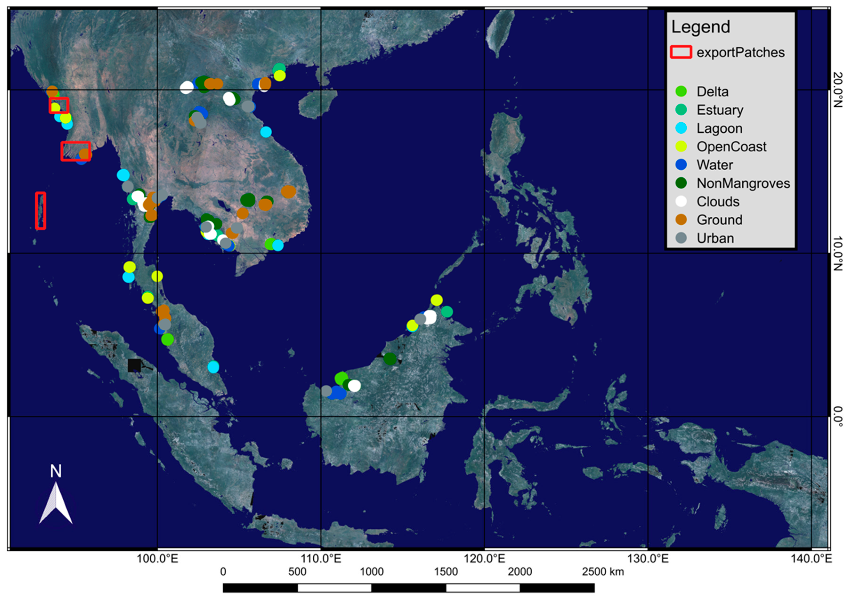[9], a traditional machine learning (ML) classifier, such as random forest (RF), was used to produce a global baseline map of mangroves for 2010, accurately discerning mangrove forests from other forests. Other scholars have identified four types of mangroves according to their sedimentary properties: deltaic, estuarine, lagoonal, and open coast [3].

Scientists widely adopt traditional ML methods, such as support vector machines [16], k-nearest neighbour [17], and RF [10], to classify land cover types in SRSI [18]. However, researchers have recently started using methods to map mangroves from complex space-borne multi-spectral images and proposed using more sophisticated ML classifiers such as convolutional neural networks (CNNs) [15,19]. CNNs are biologically inspired ML architectures that emulate the ability of the visual cortex to decompose and recompose information through interconnected neurons, allowing recognition [20]. These architectures have several applications, from speech to medical condition recognition [21], and have excellent large-scale natural image classification performance thanks to their ability to ‘learn’ hierarchical representations [22].

In recent years, CNNs have proven to be more powerful than traditional ML methods in SRSI classification [23] because, unlike RF, they can capture the semantics of an image (spatial information) using pixel values alone [24] and are now preferred when classifying complex landcover types (LCTs), such as vegetation [18]. Nevertheless, a recurrent limitation of CNNs is the need for a considerable amount of labelled data to ‘learn’ features robustly. Labelling SRSI is an often tedious and lengthy process, and there is a limited amount of pre-labelled datasets available out there, making their use for classification tasks with CNNs challenging [25].

There are several methods for adapting CNNs to the task of classifying increasingly complex hyperspectral SRSI, such as training from scratch or using pre-trained CNNs as feature extractors [26,27]. The latter is called transfer learning (TL), and it involves using CNNs that are pre-trained on large labelled natural image datasets such as ImageNet [28] to train target SRSI [29]. 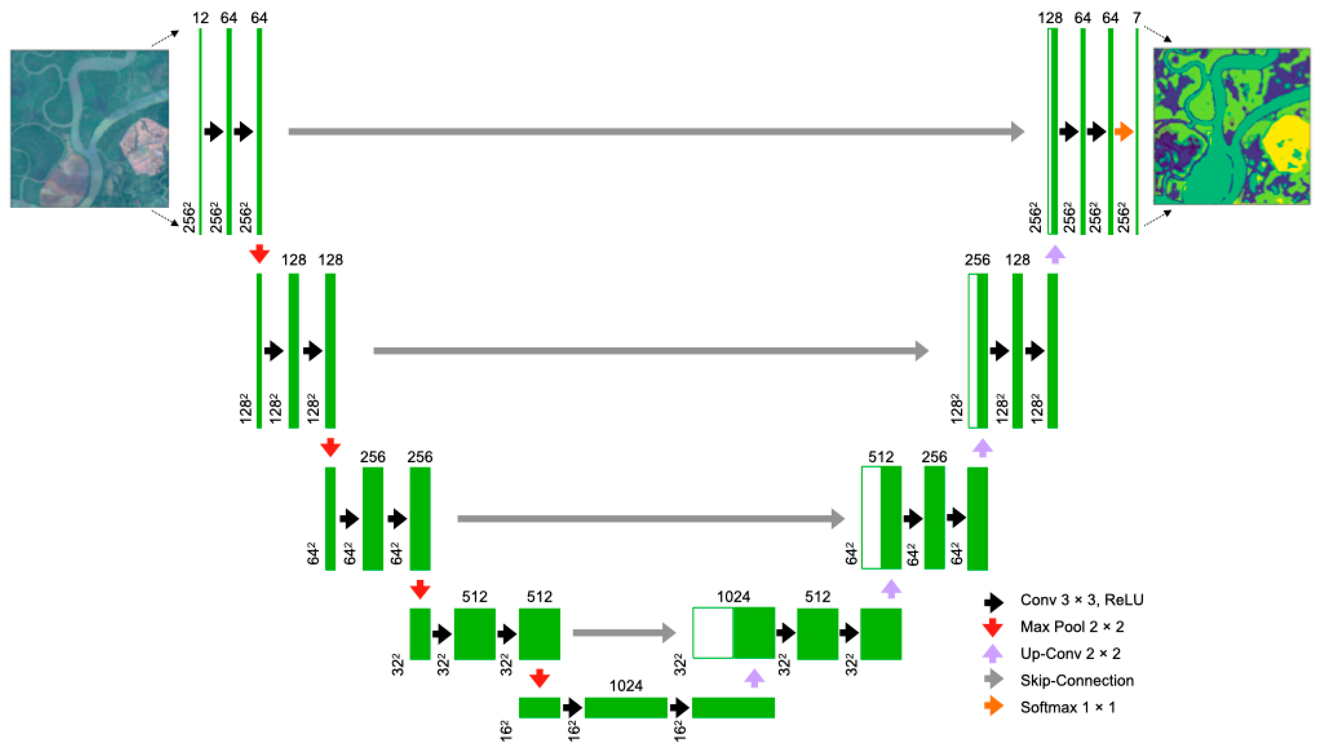This method overcomes the lack of labelled data [23] and enables CNNs to be focused on extracting the semantics of observed scenes [30]. Recently, scientists have deployed CNNs specialised in image segmentation, such as U-Net, because of their efficacy in learning the spatial relations between LCTs, especially with limited labelled images [31].

Most of the CNNs analysed demonstrated impressive SRSI classification results, many with an accuracy above 97% [29,32], but almost all were generated using powerful proprietary computers and supercomputers. Some scholars have reviewed the integration of cloud-based systems such as Google Earth Engine (GEE) and Google Collaboratory (GC) to access and classify SRSI using traditional classifiers such as RF [33,34], with some implementing classifications with CNNs [35,36]. GEE is widely used in environmental research because it stores and provides access to many SRSI datasets [32]. GC is a browser-based interface built on Jupyter Notebook’s open-source tools to support code and data visualisation [37]. It is a fairly new tool and is often used in academia to teach ML [38].

Several studies have been performed on mangrove forest mapping for SEA. One previous study has used inventories and comparisons on single- and multi-date remotely sensed datasets to identify mangrove deforestation hotspots in the region [11]. There are studies that demonstrated the utility of GEE for mapping mangroves in SEA, including one that used artificial neural network (ANN) and GEE to develop a mangrove vegetation index mapper [39], and a simple tool called Google Earth Engine Mangrove Mapping Methodology [40]. Nevertheless, no studies have attempted to classify mangrove forests in SEA with CNNs using only cloud-based platforms. Furthermore, no study has used a deep learning mangrove classification pipeline to seamlessly use freely available EO data in GEE via Google Colab (GC).

Although cloud platforms may not offer as much computational power as supercomputers, there is a growing need to create accessible monitoring tools to enhance and empower local communities worldwide and meet sustainable development goals [41]. This research, therefore, aims to create a cloud-based mangrove forest monitoring framework that is computationally less intensive to implement using GEE, GC, Google Drive (GD), and Google Cloud Storage (GCS), which uses freely available earth observation data to distinguish both mangroves from non-mangrove vegetation and map different mangrove typologies. Through this framework, local communities can generate new training data by computing new imagery and feeding them to the model. In doing so, they can use these models to assess how the local landscape is changing and determine if there are activities, such as illegal deforestation, that require tackling. Using a cloud-based system will empower local communities to perform their own monitoring, and not rely on specialists in the field, as it is an affordable resource to process large datasets [42]. Lastly, GC is a fairly new tool for developing EO-based deep learning models so the frameworks and procedures described in this study can fuel further research.

2. Materials and Methods

2.1. Software Description

2.1.1. Google Collaboratory

The project employs GC as its core platform because it offers a user-friendly interface while accessing powerful GPUs from the Google servers [38]. Additionally, using GC addresses the core limitation of CNNs, which is the need for computers with powerful GPUs to parallelise the training process. Nevertheless, CNNs can be trained using CPU power, but the process would be significantly slower [43]. GC is available in free and Pro (paid monthly) versions. The project used the latter to access the more powerful Nvidia T4 (or P100) GPUs, RAM up to 24 Gb, and get runtime limits of up to 24 h [44].

2.1.2. Monitoring Framework

The monitoring framework was split into three GC notebooks, each serving a different purpose (see Supplementary Figure S1). Splitting the workflow allows for better code maintainability and helps frame each of the notebooks as a standalone tool that does not rely on the others to operate. The user may only need, for example, to export GEE images into patches and then use them for training elsewhere or import patches from a different source and only use the framework for training or making predictions. Nonetheless, the user will need to follow the order of the notebooks if wishing to use the entire workflow. The monitoring framework prioritises using GD over GCS due to the latter having higher maintenance costs. The user, however, may use either cloud storage because the framework supports both.

2.1.3. Custom Packages

The project introduces three custom Python packages with integrated testing that have the task of unifying, standardising, and simplifying some of the most common methods of integrating GEE with GC and TensorFlow (TF), aiming to improve the reproducibility of the workflow (

Table 1. Details of the custom packages introduced in the project.

Package Name	Version	Language	Description
eeCustomTools	0.1.0	Python 3	Support for satellite imagery classification through computation of spectral indices, image segmentation, and cloud masking for Sentinel-2, Landsat-5, Landsat-7, and Landsat-8 sensors.
eeCustomDeepTools	0.1.0	Python 3	Support for manipulating and converting TFRecords exported through Google Earth Engine into batches ready for training using Keras.
CustomNeuralNetworks	0.1.0	Python 3	Implementation of custom Keras Neural Networks.

). Some of the most important tasks include adapting GEE’s JavaScript backend to its Python API for GC implementations, allowing for seamless interchangeability between Sentinel-2 and Landsat-5, Landsat-7, and Landsat-8 sensors. The packages also provide a single solution to implementing the multitude of methods to integrate ML in GC using TF and TFRecords patches exported from GEE, many of which are proposed by Google [45]. Most of these methods were considered too short or not well-documented, especially for a beginner user, and they all failed to execute multi-class classification tasks in a reproducible way (i.e., they only worked for the examples provided).

2.1.4. Code Metadata

The project was developed in Python 3.8 using Jupyter Notebooks and Visual Studio Code on a Macintosh computer and JavaScript on the GEE browser-based platform. Although the project does not rely on platforms outside the generated workflow, some parts required using GEE’s interactive tool to draw the export areas and drop points to identify the LCTs around SEA. Unfortunately, this process was not possible directly in GC due to limitations of the GEE Python API for GC when the project was carried out, but recent updates of the geemap package (see below) have made this possible now.

Python modules such as json, subprocess, and pathlib were used to access TFRecords from the target storage. The ee and geemap packages were used to access GEE’s Python API (the former) and output GEE maps (the latter). TensorFlow was the core library to implement the ML workflow using TFRecords exported from GEE. Keras is the API with a TF backend that enabled the generation and training of CNNs. The packages matplotlib, numpy, and pprint were used for visualisation purposes (numpy enabled the TFRecords files to be converted to arrays and facilitated plotting). Finally, the google.colab package was used to enable users to access target GD or GCS. Although users are strongly encouraged to use the monitoring framework online, it may also be used on a local machine using Jupyter Notebooks, with some caveats (i.e., accessing GD and GCS from within the Notebook will no longer be possible). Ultimately, the only requirement for using GC is an internet connection and an up-to-date version of one’s preferred web browser (Google suggests using Chrome, Safari, or Firefox) [46].

2.2. Study Area

The project uses the median pixel values of Sentinel-2 (S2) multi-spectral images between January and December 2016 (Figure 1). S2 was preferred to Landsat sensors because of its finer spatial resolution (10 m for blue, green, red, and NIR bands and 20 m for other bands, as opposed to 30–60 m with Landsat) as it is regarded as an essential feature to detecting subtle differences between LCTs in complex SRSI [15].

2.3. Random Forest Classification

The first stage of the preliminary classification identified single points (latitude/longitude coordinate couples) for each of the nine LCTs using GEE’s online-based interactive map (listed in Supplementary Figure S2). The identification process was performed using the median image for 2016 to align with the year used by Worthington et al. [3], to produce the mangroves’ shapefiles baseline. The process selected an average of 20 points for each of the 9 LCTs in different countries of SEA to account for different lighting conditions and the non-homogenous count of mangroves’ shapefile, for a total of 1080 points (

Table 2. Number of mangroves’ shapefiles used in each country within the area of interest (AOI) (left panel) and points used for each of the classes identified in each country (right panel). Philippines and Indonesia were not used due to the complexity and small size of their respective countries’ boundaries, making image processing and class identification challenging. The number of points for each class was kept constant at twenty, where possible (some countries did not have some of the mangroves’ typologies, or the shapefiles were too small), to overcome the imbalance in mangroves’ shapefiles count in each country.

Mangroves’ Shapefiles Used within the AOI *					Number of Points for Each Class Identified in Each Country
	Delta	Estuary	Lagoon	Open Coast	Delta	Estuary	Lagoon	Open Coast	Water	Non-Mangrove	Cloud	Ground	Urban
Cambodia	0	7	3	8	0	20	20	20	20	20	20	20	20
Laos	0	0	0	0	0	0	0	0	20	20	20	20	20
Malaysia	8	48	10	58	30	30	30	30	20	20	20	20	30
Myanmar	4	20	11	33	30	30	30	30	25	20	20	20	10
Philippines	-	-	-	-	-	-	-	-	-	-	-	-	-
Indonesia	-	-	-	-	-	-	-	-	-	-	-	-	-
Thailand	1	31	6	40	30	20	20	20	15	20	20	20	20
Vietnam	2	10	3	17	30	20	20	20	20	20	20	20	20
Total in AOI **	90	946	628	2509	120	120	120	120	120	120	120	120	120

* The AOI is the whole image in Figure 1. ** Total number of mangroves’ shapefiles from Worthington et al. [3] within the AOI.

). Although the identified points covered a large area, they were all close to the equator, and the potentially different field of view of the Sentinel-2 sensor when the images were captured was not considered an issue, as it would have affected the points equally. Furthermore, buffers were computed around each point (5 m for clouds and 50 m for the rest, due to clouds covering smaller areas) to gather additional pixels to attribute to each of the LCTs. Ultimately, it is worth noting (this is explained further in Section 2.7) that after an initial exploratory training phase, the classes were dropped from nine to seven, combining urban, clouds, and ground LCTs into a single class.

The second stage was to segment the median image composite using simple non-iterative clustering, which divides an image into spectrally different small regions to improve classification performance [47]. Finally, the entire scene was classified by feeding the segmented multi-band image to a standard RF classifier algorithm using 200 independent decision tree classifiers for each pixel [48]. The classification used 21 bands, including 12 spectral bands (B1–B12) and 9 spectral indices (Figure S2). The classification values were stored as an additional band called ‘classification’ to the base median image composite for a total of 22 bands.

A grid was applied to the image to obtain patches of 256 × 256 pixels to align with the literature [49]. Only patches contained within the Export Areas (shown in Figure 1) were exported onto GD as TFRecords to avoid exceeding the memory allowed in GEE for a single process, obtaining a total of 48,786 patches.

2.4. Convolutional Neural Networks

The project proposes the U-Net architecture to perform the multi-class classification of SRSI (Figure 2). U-Net was originally designed for binary segmentation in medical imagery [50] to generate results with a small number of labelled data [51]. Nonetheless, U-Net has since become a standard in densely labelled SRSI [52], demonstrating superior performance over other CNNs and adapting well to multi-class classification tasks [24,53]. The U-Net architecture used here diverges from what was first proposed by Ronneberger et al. [50], emulating the U-Net architectures used in SRSI classifications [49,54].

The left side of the proposed U-Net encodes the image through convolutions and max-pools operations into (semantic) feature representations at multiple levels, followed by ReLU activation functions. The right side decodes the image through up-sampling operations, concatenating the learned semantics and projecting it in higher resolutions to obtain a dense classification through a probability distribution [51]. The skip-connections enable the model to compare the encoded image to its decoded counterpart and only use the pixels with the highest probability of being correctly classified (Figure 2). The final layer is a convolution that uses a SoftMax function to obtain a multi-class probability distribution and generate a single-channel (band) image with a user-defined number of classes (here, seven). A difference with the original U-Net [50] is the presence of batch normalisations before each ReLU activation.

The U-Net architecture in Figure 2 was trained from scratch (called U-Net hereafter) (i.e., the model is yet to produce any weights that represent the ‘learned’ features) using the dataset of 48,786 patches of size 256 × 256 pixels exported from GEE, but only using the 12 spectral bands in the input images (B1–B12) (the user, however, can use an arbitrary number of bands). Additionally, to evaluate the strength of the proposed model, this was compared to two other U-Nets that used VGG19 [55] and ResNet50 [56] as feature extractors (or encoders), which replaced the left-hand side structure of Figure 2 (called VGG19 and ResNet50 moving forward). VGG19 and ResNet50 were used with weights pre-trained on ImageNet to understand the adaptability of TL to complex SRSI segmentation tasks. However, using pre-trained models limited the number of bands used for the training to three (see Section 4 for an explanation of the limitations). It was then decided to use bands B3, B4 and B8, in combination, to exploit the near-infrared region to discern vegetation better using the characteristic red edge of plants. Mangroves can be easily distinguished from other land covers such as ground and water using this spectral feature, which is unique to plants [39]. Ultimately, spectral indices were not fed to any of the models because studies found that they do not improve the accuracy of the models, as they can be directly extracted from the data [24].

2.5. Hyperparameters Search

Although most studies agree with using the categorical cross-entropy for U-Net classification tasks, often using weights to compensate for imbalanced data [50,51,57], the task of obtaining weights for TFRecords was not as straightforward. TFRecords cannot be handled like tensors or arrays, and they can only be controlled in ‘batches’ (stacks) of data. The dataset could not be explored to understand the recurrence of a class unless it was converted into tensors or arrays, which was not, however, computationally feasible. Ultimately, it was decided to use the recently developed Focal Loss (FL) function, designed to downweigh well-classified categories and ‘focus’ on those not-well-classified to compensate for the categorical imbalance [58]. In other words, if a single 256 × 256 patch had 90% of the class ‘non-mangroves’, and only 10% of the class ‘delta’, then the FL function would focus more on the latter to unpack its semantics. FL is available in the TF addons library as ‘SigmoidFocalCrossEntropy’ [59]. The FL function is defined by the equation:

$$FL\left(p_t\right)=-{\alpha }_t{\left(1-p_t\right)}^{\gamma }\log \left(p_t\right),$$

(1)

where $\gamma$ is the focusing parameter that downweighs well-classified samples, whereas $\alpha$ is a regularisation parameter that stabilises the loss [58]. Scientists have compared FL to other loss functions and demonstrated its superiority [60] and promising performance in U-Net models [61].

The optimiser of choice was the Adaptive Moment Estimation (Adam), which combines an adaptive learning rate (LR) (step size down the loss landscape) with a momentum (a parameter that controls the steepness of the gradient) [62]. The optimiser is defined as:

$${\theta }_{t+1}={\theta }_t-\frac{\eta }{\sqrt{{\widehat{\nu }}_t}+\epsilon }\widehat{m_t},$$

(2)

where $\theta$ is the parameter, $\eta$ is the LR $\widehat{\nu }$ and $\widehat{ m}$ are the first (mean) and second (variance) momentum, and $\epsilon$ is the error term [31,62,63]. The adaptive LR makes Adam an efficient optimiser in image segmentation tasks with U-Net [31]. The LR was tested as 0.001 (default) and 0.0001, and the batch size was set to 12.

2.6. Accuracy Assessment

The performance of the RF classifier run in GEE was assessed using a confusion matrix, producer and user accuracies, and kappa coefficient. The producer accuracy determines the probability that the classified samples represent that category on the ground. The user accuracy determines the probability of the samples to be correctly classified. Finally, the Kappa coefficient determines the overall accuracy of the classification. All three coefficients provide a percentage of numbers between 0 and 1 [15,64]. The RF classifier was trained using a 70–30% training–test split, whereas the deep models were trained using an 80-10-10% split. The splitting process ensured the use of ‘unseen’ data to validate the performance of the classifiers.

The performances of the deep models were also evaluated using the loss, the F1-score (the harmonic average of precision and recall), and the categorical accuracy (CA) metrics, similar to other studies [24,53,65]. F1-score is defined as:

$$F1=2\ast \frac{Precision\ast Recall}{Precision+Recall},$$

(3)

where Precision is the ratio of correctly predicted classes among all the predicted classes, while Recall is the ratio of correctly classified classes out of all predicted classes [49]. The F1-score was the preferred metric to identify the best-performing models because it accounts for false negatives and false positives, which was deemed more important in a classification problem where the classes are imbalanced. The CA is expressed as the percentage of classified pixels that match the original classification (i.e., the classification of the RF classifier) [66], accounting for true positives and true negatives. The CA metric was only used to explain the performance of the models.

Finally, the deep models were tested on a small arbitrarily chosen area of size 12 × 256 × 256 pixels and evaluated on the single classes using user and producer accuracies.

2.7. Training Process

The study trained 30 models for over 480 h of cumulative GC runtime. First, the analysis began training the U-Net using all the nine classes in Figure 2. However, it was immediately apparent that the number of classes was too large for the models to learn the semantics of the scene effectively and efficiently, probably due to its complexity. Therefore, it was decided to use seven classes instead: the four mangrove typologies, ‘water’, ‘non-mangroves’, and ‘others’ (clouds, ground, and urban combined).

The models regularly reached the 24 h GC Pro runtime limit, only training for 7 epochs at maximum in a single runtime. The runtime limit was not an issue, as the models were saved onto GD at each epoch using the ModelCheckPoint method within the Keras API [67]. The method enabled the models to be loaded and continue the training in a new runtime. Nevertheless, each model saved at every epoch was over 350 Mb, resulting in a total of 2.5 Gb of space in GD for 7 epochs. Since the project aimed to emulate a near-real-time monitoring tool with minimal budget requirements (only 15 Gb are free in GD), it was decided to evaluate and compare the performances of the models trained on only seven epochs to evaluate the accuracy of short training sessions.

3. Results

3.1. Performance Comparisons

The RF classifier in GEE showed very high accuracy for both the user and producer, with an overall accuracy of k = 0.997 (

Table 3. Confusion matrix of the random forest classifier, with relative producer and user accuracies and kappa coefficient. The accuracy was assessed on a 70–30 split between the training and the test set.

	Delta	Estuary	Lagoon	Open Coast	Water	Non-Mangrove	Others	Producer
	2716	0	0	0	0	0	0	1.00
	0	2689	0	0	0	0	0	1.00
	0	0	2591	0	0	0	0	1.00
	0	0	0	2619	0	0	0	1.00
	9	0	0	0	2336	0	2	0.995
	0	0	0	0	0	2168	0	1.00
	30	1	0	0	0	2	5100	0.994
User	0.986	0.999	1.00	1.00	1.00	0.999	0.999	k = 0.997

). The result was significant because it ensured that the accuracy assessment of the deep models was based on a very accurate preliminary pixel-wise classification using the traditional RF method.

As for the deep models, U-Net showed the lowest loss and the highest F1-score and CA overall. All the models reached the lowest loss on the validation sets at epoch seven, with loss = 0.068, 0.099, and 0.121 for U-Net, VGG-19, and ResNet50, respectively, showing no signs of overfitting (Figure 3). Overfitting occurs when the model fits the training set ‘too well’, causing an increase in the generalisation error (i.e., the model stops learning) [68].

The lack of overfitting may be due to the number of filters used in the network, which were fewer than what was originally used by Ronneberger et al. [50]. Scholars have observed a positive correlation between the number of filters and the chance for the model to lose information [49]. Additionally, batch normalisation helps avoid overfitting by regularising the loss [65]. Despite the presence of skip-connections, which helps ‘smooth’ the loss [63], the loss for the VGG19 and ResNet50 was problematic at times (Figure 3). The issue was possibly due to the complexity of the loss-landscapes [63], which was expected due to the heterogeneity of the scene. The complexity may have hindered the segmentation task [30] and led the models to dwell in ‘local minima’. The issue indeed persisted using a smaller LR (0.0001) [68].

Across all the epochs, the best models (i.e., those with the highest F1-score on the validation set) were at epochs six, seven, and four, for U-Net, VGG19, and ResNet50, respectively (

Table 4. Metrics of the best-performing models according to the F1-scores for the validation sets (rows in bold). The datasets were split as 80-10-10% for the training, validation, and test sets, respectively.

Model	Epoch	Dataset	Loss	Precision	Recall	F1-Score	Accuracy
U-Net	6	Training	0.043	0.989	0.840	0.908	0.932
		Validation	0.068	0.961	0.668	0.788	0.907
		Test	0.062	0.981	0.645	0.778	0.910
VGG19	7	Training	0.044	0.990	0.827	0.901	0.930
		Validation	0.100	0.987	0.676	0.803	0.894
		Test	0.100	0.988	0.261	0.412	0.896
ResNet50	4	Training	0.035	0.993	0.876	0.931	0.948
		Validation	0.125	0.990	0.543	0.701	0.732
		Test	0.127	0.993	0.542	0.701	0.725

). The metrics analysis showed that U-Net and ResNet50 maintained an F1-score above 0.7 across training, validation, and test sets, whereas VGG19 dropped the F1-score dramatically on the test set. The result eloquently demonstrates that VGG19 struggled to identify the false negatives and positives when tested on unseen data. On the other hand, unsurprisingly, CA showed very high values for all the models, probably inflated because the metric ignores data imbalance [66].

The loss showed low values for all the models. However, this is both a strength and a limitation. It is a strength because it demonstrates that the models could navigate the loss landscape and find ‘local minima’ and allow for reliable predictions. On the other hand, it is a limitation because it means that the models could not be trained for more epochs without risking overfitting the data [68]. The U-Net model showed the lowest losses, probably thanks to its ability to ingest any number of channels (bands) for the input images, as opposed to only three for VGG19 and ResNet50. The precision metric revealed very high values across the models, demonstrating the ability of the models to distinguish between true and false positives. However, the recall metric proved that both VGG19 and ResNet50 suffered from the weight of false negatives. U-Net was the only model that ‘passed’ the accuracy assessment, showcasing good predictive ability across the board.

The results were confirmed by visualising the classification of the test set for each of the models as the epochs progressed. The U-Net demonstrated to be capable of learning the semantics of the images and discerning between different classes very well, explaining the high F1-score obtained on the test set (Figure 4A). On the other hand, VGG19 and ResNet50 struggled to learn semantics and discern between classes. The progression of the epochs (Figure 4B,C) reflects what is seen in Figure 3B,C, where the loss and the F1-score fluctuated. It seemed that the models may have needed a few more epochs of training to capture the complexity of the scenes. Nonetheless, the loss values did not show much room for improvement without the risk of overfitting.

When analysing the classification performance at the class level of the best-performing models through producer and user accuracies, it was evident that the positive metrics seen so far were driven mainly by the correct classification of non-mangrove classes (

Table 5. User and producer accuracies of the deep models which scored the highest F1-score on the validation sets.

		Epoch	Delta	Estuary	Lagoon	Open Coast	Water	Non-Mangroves	Other
U-Net	User	6	0.044	0.244	0.00	0.00	0.529	0.868	0.493
	Producer		0.165	0.361	0.00	0.00	0.350	0.055	0.498
VGG19	User	7	0.008	0.00	0.00	0.00	0.197	0.963	0.931
	Producer		0.209	0.146	0.00	0.00	0.498	0.211	0.264
ResNet50	User	4	0.00	0.011	0.006	0.00	0.333	0.903	0.117
	Producer		0.00	0.187	0.103	0.00	0.372	0.148	0.372

). To that end, mangrove typologies, particularly lagoon and open coast, were poorly classified by all models, with U-Net showing slightly better accuracies. This issue may be linked to the high spectral similarities between mangrove typologies and the significant intra-class heterogeneity in the SRSI [26]. After all, the differentiation between mangrove typologies by Worthington et al. [3] was mainly based on sedimentology rather than the plant’s canopy structure, meaning that the mangroves may very well look alike from space, both optically and spectrally. Moreover, mangroves’ dense canopy does not allow them to discern the soil’s structure beneath them.

The inability of VGG19 and ResNet50 to classify water correctly was somewhat surprising. This is because the models employed in the study are designed to better interpret the semantics of the images and the shapes/outlines of the objects in them, which are very distinct for water bodies. However, this was isolated to VGG19 and ResNet50 because both U-Net and the preliminary classification using RF distinguished water bodies well. Furthermore, the ‘non-mangroves’ class was the best-classified category across all models. This was expected because the plant’s spectral features are very distinct [39]. Finally, the class ‘other’ (i.e., clouds, ground, urban) was best classified by the VGG19 model. However, this may have been a product of the failure in segmenting the rest of the features in the SRSI, as seen in Figure 4B.

U-Net was the ‘most balanced’ model, discerning between more classes than VGG19 and ResNet50 and segmenting the images better. Nevertheless, the model failed to capture the differences between mangrove typologies, which may be an issue unrelated to the model (as discussed earlier).

3.2. Spatial-Temporal Performance of U-Net

Given that the U-Net was the best-performing model of the study, it was decided to test its adaptability and performance in a multi-year classification task. Although the model showed poor performance in classifying mangrove classes, it showed promising results with the rest of the classes. This was evident when merging the classified patches into a single scene for an arbitrary target area (Figure 5, 2016 and

Table 6. Confusion matrices with relative user and producer accuracies produced using U-Net for the 2016 classified image.

	Delta	Estuary	Lagoon	Open Coast	Water	Non-Mangrove	Others	Producer
	4611	23,548	0	0	35,982	21,626	19,398	0.044
	10,836	55,274	0	0	72,801	51,592	36,145	0.244
	1169	6237	0	0	9154	5059	6566	0
	1768	10,660	0	0	14,958	8835	9226	0
	6524	27,151	0	0	95,956	30,584	21,134	0.529
	207	3623	0	0	1887	789	2598	0.087
	2930	26,547	0	0	43,218	23,853	93,986	0.493
User	0.164	0.361	0	0	0.350	0.006	0.497

) and visually comparing it to RGB images of the same area (Figure 6, 2016). The model’s greatest strength was its ability to capture the shapes of the riverbanks, but it often confused what could be flood plains (i.e., rice fields or wet ground) with water. Nonetheless, the U-Net might have confused some mangrove typologies with non-mangrove forest. Additionally, the U-Net showed some issues at the edges of the patches (multiple squares are visible in Figure 5, 2016), although this is a known issue with U-Net models [52] that can be overcome by generating patches with overlapping pixels [24].

When the U-Net was used to classify median composite images from 2017 and 2018, it soundly failed to discern between classes (Figure 5 and Figure 6,

Table 7. Confusion matrices with relative user and producer accuracies produced using U-Net for the 2017 classified image.

	Delta	Estuary	Lagoon	Open Coast	Water	Non-Mangrove	Others	Producer
	218	440	0	0	32,371	62,378	9758	0.002
	311	420	0	0	62,132	140,710	23,075	0.002
	50	195	0	0	8794	15,501	3645	0
	47	91	0	0	13,152	26,679	5478	0
	421	1210	0	0	84,185	81,384	14,149	0.464
	5	4	0	0	1043	6613	1439	0.726
	203	346	0	0	45,499	75,688	68,798	0.361
User	0.174	0.155	0	0	0.341	0.016	0.545

and

Table 8. Confusion matrices with relative user and producer accuracies produced using U-Net for the 2018 classified image.

	Delta	Estuary	Lagoon	Open Coast	Water	Non-Mangrove	Others	Producer
	306	438	0	0	38,538	50,112	15,771	0.003
	582	1103	0	0	73,624	119,179	32,160	0.005
	60	102	0	0	10,308	12,935	4780	0
	74	193	0	0	15,974	21,629	7577	0
	491	1496	0	0	95,223	68,422	15,717	0.525
	25	74	0	0	1273	3173	4559	0.349
	294	637	0	0	57,315	50,652	81,636	0.428
User	0.167	0.273	0	0	0.326	0.010	0.503

). The model could distinguish between the class other and the rest of the classes, but it could not capture the differences between mangrove and non-mangrove forests, and it could not segment water bodies properly (i.e., rivers were mostly ignored). The inability to segment waterbodies was unexpected, especially considering that these, particularly the larger ones, are mostly similar across the three median-values images (Figure 6). The issue may be due to the interannual variability of plant phenology, which is known to vary with changing climatic conditions, water availability, and seasonality [2]. These last two factors are especially relevant along riverbanks in SEA due to the impact of both rainfall and distinct high- and low-tide ranges’ variability over time [69]. Tides play a crucial role in the identification of mangroves from space, as they can often be inundated and look spectrally similar to water, even if the canopy stands above it. The spectral reflectance of the canopy can effectively be altered by the presence of more suspended sediments and water beneath [70]. Additionally, saturated ground can too be spectrally similar to water. Moreover, light conditions, water vapour, and pollutants in the atmosphere may have distorted the reflectance of bodies on the ground. Ultimately, other unknown underlying processes may have altered the spectral properties of the features in the images (e.g., drought, lower groundwater recharge, lower salinity).

4. Discussion

The use of GC was surprisingly stable throughout the project, and any drop in the internet connection (provided they were not for too long) did not lead to runtime failures and affected the completion of the training. The stability of GC is an essential aspect of the platform, particularly when the internet connection is not consistently stable. Although the cost of GC’s Pro version is low, the project has indirectly shown that using GC’s free version would not be feasible for a particularly intensive task. This is true unless the user is comfortable with consistently saving and picking up the training multiple times, has a large amount of Google Storage available (which has a monetary cost), and can wait for Google to allow for another training session. Unfortunately, there is no way of saying when the server will be ‘free enough’ to let a free user start training sessions again.

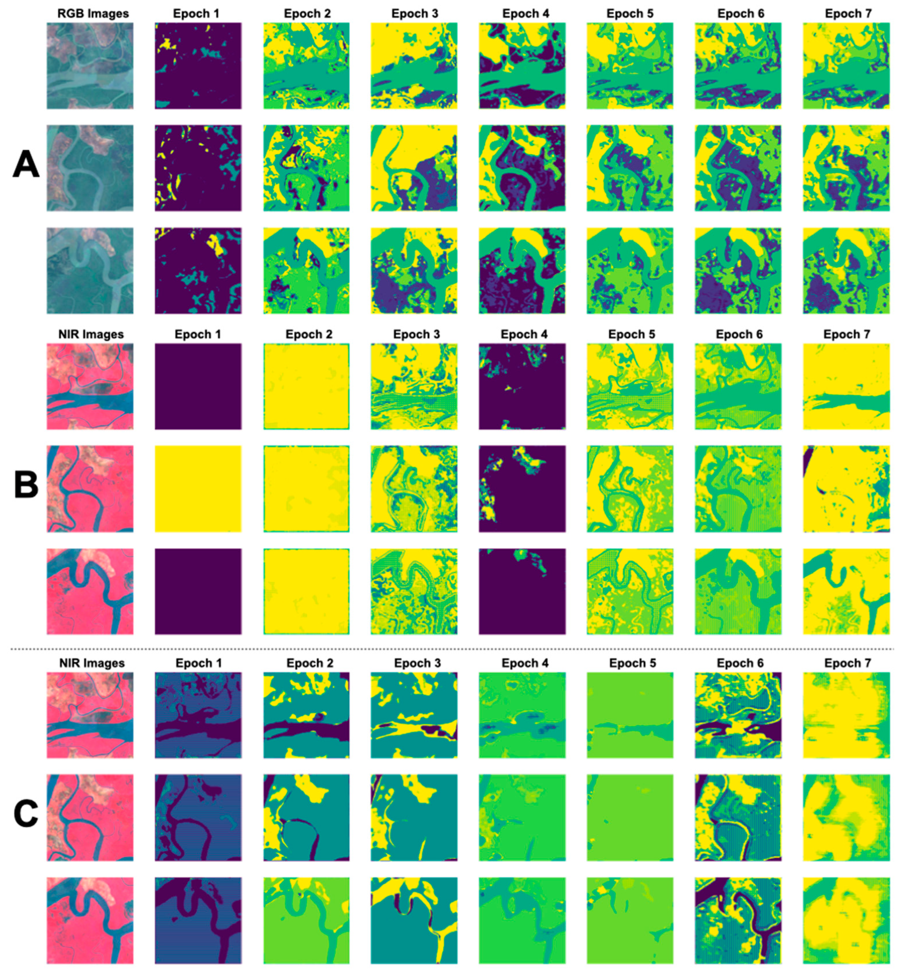
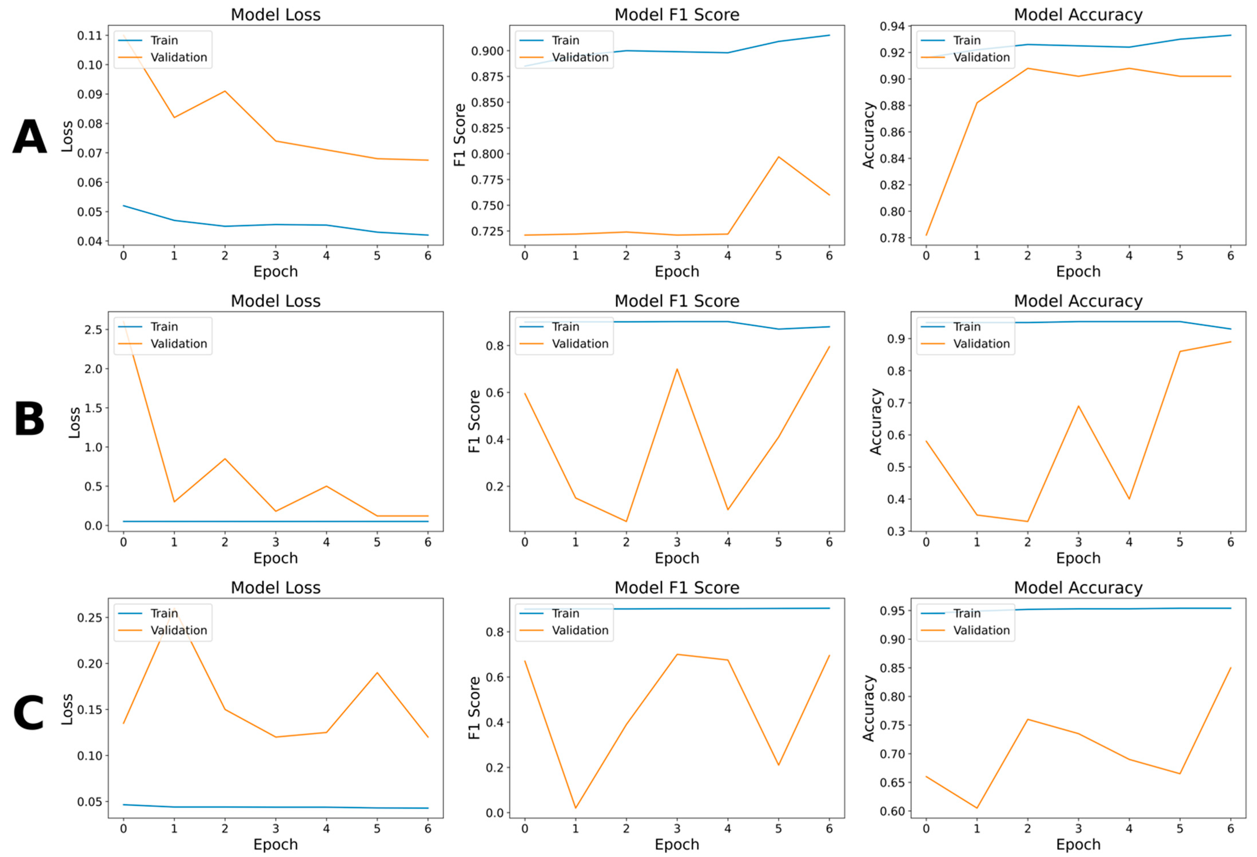
The project has revealed substantial differences between the U-Net model and VGG19 and ResNet50, demonstrating that TL was not appropriate for such a complex classification task. Although all the models failed to classify some mangrove classes, VGG19 and ResNet50 showed an evident inability to segment the images (Figure 4B,C). Some scholars argue that pre-trained models contain unnecessary information for classifying highly variable SRSI [71,72] and that the use of pre-trained models as feature extractors is best-suited for small-scale datasets [26]. Furthermore, the VGG19 and ResNet50 models could only accept three bands if used with pre-trained weights, potentially losing meaningful SRSI semantics and spectral properties.

The use of seven classes may have overwhelmed the models and identifying fewer classes could improve the results. Some scientists, for example, argue that generating a model for each of the target classes increases the classification accuracy, especially when the scene presents unbalanced distributions of LCTs [53]. Moreover, given that distinguishing between mangrove typologies was particularly challenging, it may be helpful and may lead to better results to group all mangrove classes into one and maintain the rest as separate (i.e., mangroves, water, non-mangroves, clouds, ground, urban classes).

The pixel-wise classification performed with the RF classifier may have some design issues because the classes were manually identified using a median image composite for a single year. It is evident that selecting the image with which to perform the preliminary classification using RF classifiers (or other ML algorithms) and create training patches requires careful considerations, and using median composite of images captured over a whole year may not be ideal due to the dynamicity of land surfaces [34]. Seasonality and water availability have a considerable effect on the spectral reflectance of land features, and training classifiers using images of the same year that account for the changes of LCTs over time in the training datasets could lead to more reliable preliminary classifications. To that end, and especially if mapping coastal environments such as mangrove forests, including images with different tide dynamics may help the models to better discern between mangroves and water, allowing to capture features otherwise ‘hidden’ if using median pixel values. Some scholars have developed the Submerged Mangrove Recognition Index (SMRI) using the high-resolution Gaofen satellite to assess the effects of tides across the year, coupling images captured at different tide heights and correcting the classification according to the detected differences and informing on the actual spatial distribution of mangroves [73]. Nevertheless, while adding SMRI to the bands of the images fed to the classifier could better inform the models of interannual land features’ variability, it would require collecting significant EO data corresponding to high and low tides to better calibrate deep learning models.

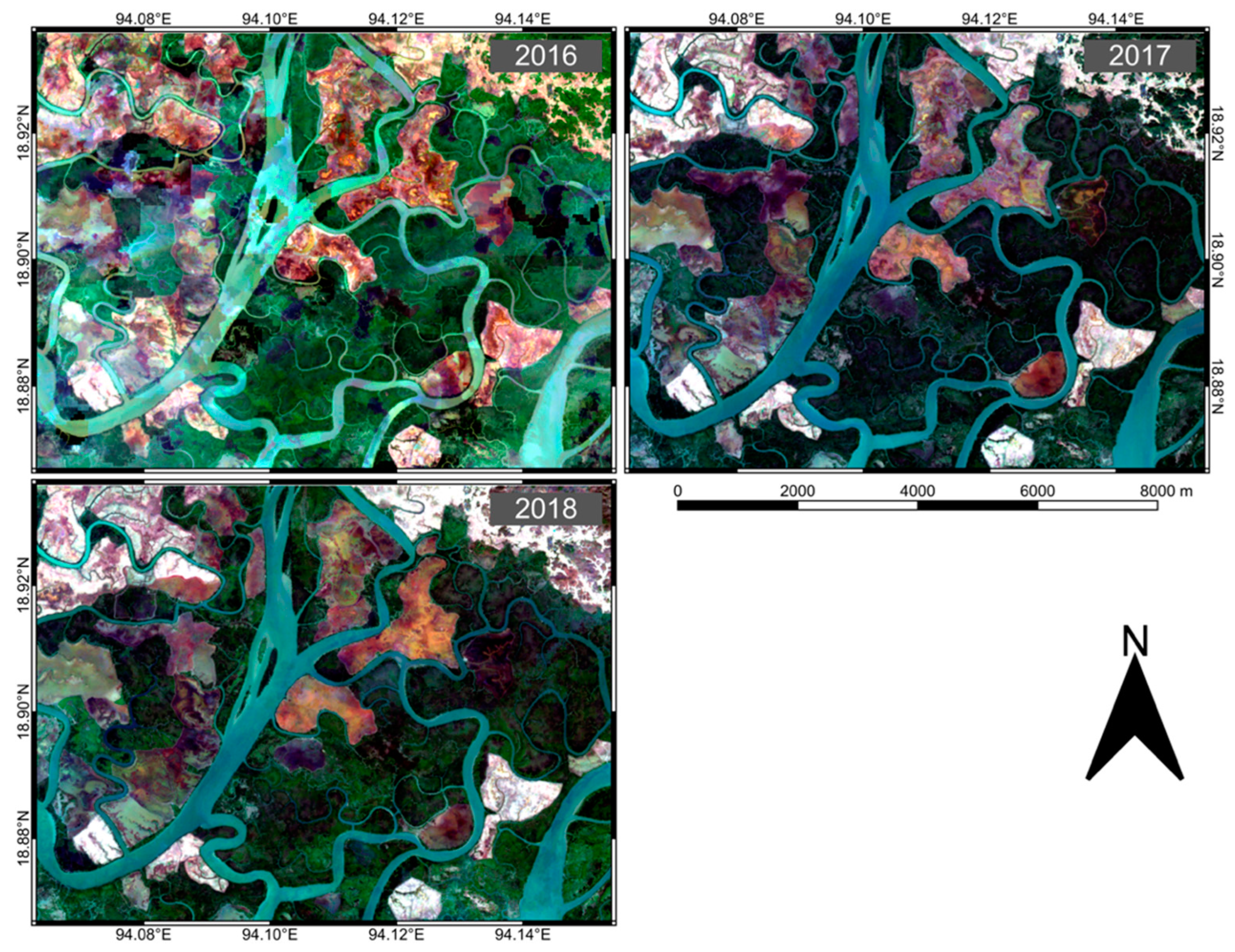
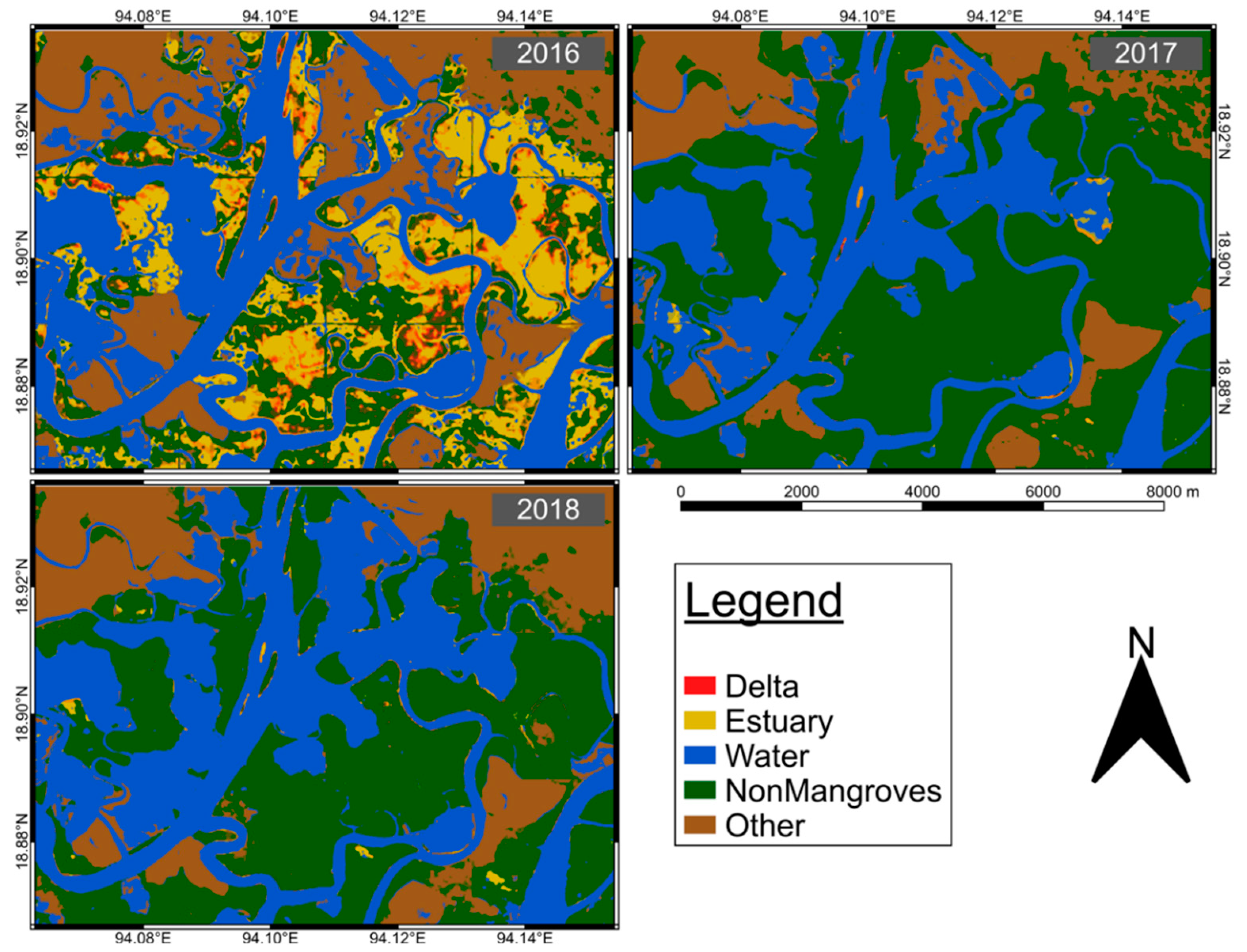
Finally, although the U-Net model could cleverly distinguish the semantics of inland LCTs that have subtle spectral differences, features on coastlines and riverbanks resulted more challenging to classify, especially due to the interaction with water. The results of the multi-year classification have demonstrated that training the U-Net model on a median pixel-value image for a single year could be both inaccurate and misleading. It could be inaccurate due to the lack of tide dynamics information (and other seasonal signatures), and misleading because it ‘forces’ the model to generate weights and learn a semantic that may not be correct. To solve the issue, it is important to not only account for interannual land features’ variability, but also to feed images of multiple years to the model to account for different environmental conditions that may alter features’ spectral reflectance over time (e.g., light conditions, sensor errors, different amounts of pollutants in the air). While testing the transferability to the SMRI computation to Sentinel and other coarser spatial resolution satellites is a worthy research endeavour, it is presently outside the scope of our research.

5. Conclusions

Mangrove deforestation jeopardises the survival of tropical coastal communities while contributing to alimenting carbon emissions worldwide. Although the growth of computing power enables scientists to develop better and more accurate monitoring tools to guide interventions, increasingly intensive tasks and complex algorithms are becoming unsuitable for commercial and personal computers.

This paper has presented a cloud-based alternative to owning proprietary supercomputers that enables anyone with a computer and an internet connection to perform complex classification tasks using Google Colab and Google Earth Engine, with the help of the proposed custom Python packages. The mangrove monitoring framework was developed as an attempt to standardise and unify some of the most used tasks to handle TFRecords in a machine learning workflow while providing thorough documentation and guidance. Moreover, the framework has explored novel image segmentation architecture such as U-Nets, comparing the strengths and weaknesses of training from scratch and fine-tuning using pre-trained VGG19 and ResNet50 as encoders to the U-Net model.

The analysis has shown that an untrained U-Net model is superior in segmenting complex satellite remote sensing images compared to U-Net using VGG19 and ResNet50 models as feature extractors. Nevertheless, although the model provided some good results, feeding too-complex semantics (i.e., different mangrove typologies) has hindered the training process and affected the results. In the future, researchers may wish to extend the current work by preliminarily classifying mangroves accounting for interannual land features’ variability, with a particular focus on the effects of tide dynamics to mangroves’ spectral signature. It will also be important to feed the model with images captured across several years to account for ongoing environmental condition changes and to consider mangroves as a single class rather than splitting them by type. In addition, the presented U-Net model could be extended by adding more layers to avoid overfitting and may also be pre-trained using one of the multi-class remote sensing imagery datasets available online (e.g., BigEarthNet—https://bigearth.net) (accessed on 1 January 2022). However, this last step needs to be taken with care if desiring to maintain storage costs and low training runtimes.

The authors believe that the proposed monitoring framework can lead the way to creating low-cost, cloud-based, open-source tools that governments, environmental agencies, and researchers can deploy to monitor mangroves (and more) in SEA and around the rest of the world.

References

1. Thomas, N.; Bunting, P.; Lucas, R.; Hardy, A.; Rosenqvist, A.; Fatoyinbo, T. Mapping mangrove extent and change: A globally applicable approach. Remote Sens. 2018, 10, 1466. [Google Scholar] [CrossRef] [Green Version]
2. Pastor-Guzman, J.; Dash, J.; Atkinson, P.M. Remote sensing of mangrove forest phenology and its environmental drivers. Remote Sens. Environ. 2018, 205, 71–84. [Google Scholar] [CrossRef] [Green Version]
3. Worthington, T.A.; zu Ermgassen, P.S.E.; Friess, D.A.; Krauss, K.W.; Lovelock, C.E.; Thorley, J.; Tingey, R.; Woodroffe, C.D.; Bunting, P.; Cormier, N.; et al. A global biophysical typology of mangroves and its relevance for ecosystem structure and deforestation. Sci. Rep. 2020, 10, 14652. [Google Scholar] [CrossRef] [PubMed]
4. Giri, C.; Ochieng, E.; Tieszen, L.L.; Zhu, Z.; Singh, A.; Loveland, T.; Masek, J.; Duke, N. Status and distribution of mangrove forests of the world using earth observation satellite data. Glob. Ecol. Biogeogr. 2011, 20, 154–159. [Google Scholar] [CrossRef]
5. Koh, H.; Teh, S.; Kh’ng, X.; Raja Barizan, R. Mangrove forests: Protection against and resilience to coastal disturbances. J. Trop. For. Sci. 2018, 30, 446–460. [Google Scholar] [CrossRef]
6. Wan, L.; Zhang, H.; Lin, G.; Lin, H. A small-patched convolutional neural network for mangrove mapping at species level using high-resolution remote-sensing image. Ann. GIS 2019, 25, 45–55. [Google Scholar] [CrossRef]
7. Hamilton, S.E.; Friess, D.A. Global carbon stocks and potential emissions due to mangrove deforestation from 2000 to 2012. Nat. Clim. Chang. 2018, 8, 240–244. [Google Scholar] [CrossRef] [Green Version]
8. Donato, D.C.; Kauffman, J.B.; Murdiyarso, D.; Kurnianto, S.; Stidham, M.; Kanninen, M. Mangroves among the most carbon-rich forests in the tropics. Nat. Geosci. 2011, 4, 293–297. [Google Scholar] [CrossRef]
9. Bunting, P.; Rosenqvist, A.; Lucas, R.M.; Rebelo, L.M.; Hilarides, L.; Thomas, N.; Hardy, A.; Itoh, T.; Shimada, M.; Finlayson, C.M. The global mangrove watch—A new 2010 global baseline of mangrove extent. Remote Sens. 2018, 10, 1669. [Google Scholar] [CrossRef] [Green Version]
10. Richards, D.R.; Friess, D.A. Rates and drivers of mangrove deforestation in Southeast Asia, 2000–2012. Proc. Natl. Acad. Sci. USA 2016, 113, 344–349. [Google Scholar] [CrossRef] [Green Version]
11. Gandhi, S.; Jones, T.G. Identifying mangrove deforestation hotspots in South Asia, Southeast Asia and Asia-Pacific. Remote Sens. 2019, 11, 728. [Google Scholar] [CrossRef] [Green Version]
12. Akber, M.A.; Aziz, A.A.; Lovelock, C. Major drivers of coastal aquaculture expansion in Southeast Asia. Ocean Coast. Manag. 2020, 198, 105364. [Google Scholar] [CrossRef]
13. Climate Change 2021: The Physical Science Basis. Available online: https://www.ipcc.ch/report/ar6/wg1/downloads/report/IPCC_AR6_WGI_Full_Report.pdf (accessed on 1 January 2022).
14. Wang, L.; Jia, M.; Yin, D.; Tian, J. A review of remote sensing for mangrove forests: 1956–2018. Remote Sens. Environ. 2019, 231, 111223. [Google Scholar] [CrossRef]
15. Liu, X.; Fatoyinbo, T.E.; Thomas, N.M.; Guan, W.W.; Zhan, Y.; Mondal, P.; Lagomasino, D.; Simard, M.; Trettin, C.C.; Deo, R.; et al. Large-Scale High-Resolution Coastal Mangrove Forests Mapping across West Africa with Machine Learning Ensemble and Satellite Big Data. Front. Earth Sci. 2021, 8, 560933. [Google Scholar] [CrossRef]
16. Sonobe, R.; Yamaya, Y.; Tani, H.; Wang, X.; Kobayashi, N.; Mochizuki, K. Crop classification from Sentinel-2-derived vegetation indices using ensemble learning. J. Appl. Remote Sens. 2018, 12, 026019. [Google Scholar] [CrossRef] [Green Version]
17. Zhang, L.; Zhang, L.; Du, B. Deep learning for remote sensing data: A technical tutorial on the state of the art. IEEE Geosci. Remote Sens. Mag. 2016, 4, 22–40. [Google Scholar] [CrossRef]
18. Gu, Y.; Wang, Y.; Li, Y. A survey on deep learning-driven remote sensing image scene understanding: Scene classification, scene retrieval and scene-guided object detection. Appl. Sci. 2019, 9, 2110. [Google Scholar] [CrossRef] [Green Version]
19. Li, Q.; Wong, F.K.K.; Fung, T. Mapping multi-layered mangroves from multispectral, hyperspectral, and LiDAR data. Remote Sens. Environ. 2021, 258, 112403. [Google Scholar] [CrossRef]
20. Lecun, Y.; Bengio, Y.; Hinton, G. Deep learning. Nature 2015, 521, 436–444. [Google Scholar] [CrossRef]
21. Alom, M.Z.; Taha, T.M.; Yakopcic, C.; Westberg, S.; Sidike, P.; Nasrin, M.S.; Van Essen, B.C.; Awwal, A.A.S.; Asari, V.K. The History Began from AlexNet: A Comprehensive Survey on Deep Learning Approaches. Available online: http://arxiv.org/abs/1803.01164 (accessed on 1 January 2022).
22. Chaib, S.; Liu, H.; Gu, Y.; Yao, H. Deep Feature Fusion for VHR Remote. IEEE Trans. Geosci. Remote Sens. 2017, 55, 4775–4784. [Google Scholar] [CrossRef]
23. Hu, F.; Xia, G.S.; Hu, J.; Zhang, L. Transferring deep convolutional neural networks for the scene classification of high-resolution remote sensing imagery. Remote Sens. 2015, 7, 14680–14707. [Google Scholar] [CrossRef] [Green Version]
24. Stoian, A.; Poulain, V.; Inglada, J.; Poughon, V.; Derksen, D. Land cover maps production with high resolution satellite image time series and convolutional neural networks: Adaptations and limits for operational systems. Remote Sens. 2019, 11, 1986. [Google Scholar] [CrossRef] [Green Version]
25. Nogueira, K.; Penatti, O.A.B.; dos Santos, J.A. Towards better exploiting convolutional neural networks for remote sensing scene classification. Pattern Recognit. 2017, 61, 539–556. [Google Scholar] [CrossRef] [Green Version]
26. Cheng, G.; Xie, X.; Han, J.; Guo, L.; Xia, G.S. Remote Sensing Image Scene Classification Meets Deep Learning: Challenges, Methods, Benchmarks, and Opportunities. IEEE J. Sel. Top. Appl. Earth Obs. Remote Sens. 2020, 13, 3735–3756. [Google Scholar] [CrossRef]
27. Zhang, B.; Zhang, Y.; Wang, S. A Lightweight and Discriminative Model for Remote Sensing Scene Classification with Multidilation Pooling Module. IEEE J. Sel. Top. Appl. Earth Obs. Remote Sens. 2019, 12, 2636–2653. [Google Scholar] [CrossRef]
28. Deng, J.; Dong, W.; Socher, R.; Li-Jia, L.; Kai, L.; Fei-Fei, L. ImageNet: A large-scale hierarchical image database. In Proceedings of the 2009 IEEE Conference on Computer Vision and Pattern Recognition, Miami, FL, USA, 20–25 June 2009; pp. 248–255. [Google Scholar] [CrossRef] [Green Version]
29. Liu, Y.; Huang, C. Scene classification via triplet networks. IEEE J. Sel. Top. Appl. Earth Obs. Remote Sens. 2018, 11, 220–237. [Google Scholar] [CrossRef]
30. Ghazouani, F.; Farah, I.R.; Solaiman, B. A Multi-Level Semantic Scene Interpretation Strategy for Change Interpretation in Remote Sensing Imagery. IEEE Trans. Geosci. Remote Sens. 2019, 57, 8775–8795. [Google Scholar] [CrossRef]
31. Giang, T.L.; Dang, K.B.; Le, Q.T.; Nguyen, V.G.; Tong, S.S.; Pham, V.M. U-net convolutional networks for mining land cover classification based on high-resolution UAV imagery. IEEE Access 2020, 8, 186257–186273. [Google Scholar] [CrossRef]
32. Liu, Q.; Basu, S.; Ganguly, S.; Mukhopadhyay, S.; DiBiano, R.; Karki, M.; Nemani, R. DeepSat V2: Feature augmented convolutional neural nets for satellite image classification. Remote Sens. Lett. 2020, 11, 156–165. [Google Scholar] [CrossRef] [Green Version]
33. Tamiminia, H.; Salehi, B.; Mahdianpari, M.; Quackenbush, L.; Adeli, S.; Brisco, B. Google Earth Engine for geo-big data applications: A meta-analysis and systematic review. J. Photogramm. Remote Sens. 2020, 164, 152–170. [Google Scholar] [CrossRef]
34. Amani, M.; Ghorbanian, A.; Ahmadi, S.A.; Kakooei, M.; Moghimi, A.; Mirmazloumi, S.M.; Moghaddam, S.H.A.; Mahdavi, S.; Ghahremanloo, M.; Parsian, S.; et al. Google Earth Engine Cloud Computing Platform for Remote Sensing Big Data Applications: A Comprehensive Review. IEEE J. Sel. Top. Appl. Earth Obs. Remote Sens. 2020, 13, 5326–5350. [Google Scholar] [CrossRef]
35. Xin, Y.; Adler, P.R. Mapping Miscanthus using multi-temporal convolutional neural network and google earth engine. In Proceedings of the 3rd ACM SIGSPATIAL International Workshop on AI for Geographic Knowledge Discovery, Chicago, IL, USA, 5 November 2019; pp. 81–84. [Google Scholar] [CrossRef] [Green Version]
36. Zhang, T.; Tang, H. Evaluating the generalization ability of convolutional neural networks for built-up area extraction in different cities of China. Optoelectron. Lett. 2020, 16, 52–58. [Google Scholar] [CrossRef]
37. Randles, B.M.; Pasquetto, I.V.; Golshan, M.S.; Borgman, C.L. Sing the Jupyter Notebook as a tool for open science: An empirical study. In Proceedings of the 17th ACM/IEEE Joint Conference on Digital Libraries, Tononto, ON, Canada, 19–23 June 2017. [Google Scholar]
38. Carneiro, T.; Medeiros, R.V.; Nóbrega, D.A.; Nepomuceno, T.; Bian, G.; Albuquerque, V.H.C.D.E. Performance Analysis of Google Colaboratory as a Tool for Accelerating Deep Learning Applications. IEEE Access 2018, 6, 61677–61685. [Google Scholar] [CrossRef]
39. Baloloy, A.B.; Blanco, A.C.; Rhommel, R.; Ana, C.S.; Nadaoka, K. ISPRS Journal of Photogrammetry and Remote Sensing Development and application of a new mangrove vegetation index (MVI) for rapid and accurate mangrove mapping. ISPRS J. Photogramm. Remote Sens. 2020, 166, 95–117. [Google Scholar] [CrossRef]
40. Yancho, J.M.M.; Jones, T.G.; Gandhi, S.R.; Ferster, C.; Lin, A.; Glass, L. The google earth engine mangrove mapping methodology (Geemmm). Remote Sens. 2020, 12, 3758. [Google Scholar] [CrossRef]
41. Anderson, K.; Ryan, B.; Sonntag, W.; Kavvada, A.; Friedl, L. Earth observation in service of the 2030 Agenda for Sustainable Development. Geo-Spat. Inf. Sci. 2017, 20, 77–96. [Google Scholar] [CrossRef]
42. Younes Cárdenas, N.; Joyce, K.E.; Maier, S.W. Monitoring mangrove forests: Are we taking full advantage of technology? Int. J. Appl. Earth Obs. Geoinf. 2017, 63, 1–14. [Google Scholar] [CrossRef] [Green Version]
43. Maggiori, E.; Tarabalka, Y.; Charpiat, G.; Alliez, P.; Member, S. Convolutional Neural Networks for Large-Scale Remote Sensing Image Classification IEEE Transactions on Geoscience and Remote Sensing 1 Convolutional Neural Networks for Large-Scale Remote Sensing Image Classification. IEEE Trans. Geosci. Remote Sens. 2017, 55, 645–657. [Google Scholar] [CrossRef] [Green Version]
44. Google Google Colab Pro. Available online: https://colab.research.google.com/signup (accessed on 1 January 2022).
45. Google TensorFlow Example Workflows. Available online: https://developers.google.com/earth-en-439%0Agine/guides/tf_examples (accessed on 1 January 2022).
46. Google Collaboratory: Frequently Asked Questions. Available online: https://research.google.com/colabora-441%0Atory/faq.html (accessed on 1 January 2022).
47. Zhang, S.; Dang, R. The general planning of hospital under the concept of sustainable development. In Proceedings of the 2011 International Conference on Electric Technology and Civil Engineering (ICETCE), Lushan, China, 22–24 April 2011; pp. 5606–5608. [Google Scholar] [CrossRef]
48. Breiman, L. Random Forests. In Web Information Systems Engineering; Lecture Notes in Computer Science; WISE: London, UK, 2020; Volume 12343, pp. 503–515. [Google Scholar] [CrossRef]
49. Wagner, F.H.; Sanchez, A.; Tarabalka, Y.; Lotte, R.G.; Ferreira, M.P.; Aidar, M.P.M.; Gloor, E.; Phillips, O.L.; Aragão, L.E.O.C. Using the U-net convolutional network to map forest types and disturbance in the Atlantic rainforest with very high resolution images. Remote Sens. Ecol. Conserv. 2019, 5, 360–375. [Google Scholar] [CrossRef] [Green Version]
50. Ronneberger, O.; Fischer, P.; Brox, T. U-Net: Convolutional Networks for Biomedical Image Segmentation. Available online: http://arxiv.org/abs/1505.04597 (accessed on 1 January 2022).
51. Wang, S.; Chen, W.; Xie, S.M.; Azzari, G.; Lobell, D.B. Weakly supervised deep learning for segmentation of remote sensing imagery. Remote Sens. 2020, 12, 207. [Google Scholar] [CrossRef] [Green Version]
52. Huang, B.; Lu, K.; Audebert, N.; Khalel, A.; Tarabalka, Y.; Malof, J.; Boulch, A.; Saux, B.L.; Collins, L.; Bradbury, K.; et al. Large-scale semantic classification: Outcome of the first year of inria aerial image labeling benchmark. Int. Geosci. Remote Sens. Symp. 2018, 2018, 6947–6950. [Google Scholar] [CrossRef]
53. Ulmas, P.; Liiv, I. Segmentation of Satellite Imagery Using U-Net Models for Land Cover Classification. Available online: http://arxiv.org/abs/2003.02899 (accessed on 1 January 2022).
54. Kattenborn, T.; Eichel, J.; Fassnacht, F.E. Convolutional Neural Networks enable efficient, accurate and fine-grained segmentation of plant species and communities from high-resolution UAV imagery. Sci. Rep. 2019, 9, 17656. [Google Scholar] [CrossRef] [PubMed]
55. Simonyan, K.; Zisserman, A. Very Deep Convolutional Networks for Large-Scale Image Recognition. Available online: http://arxiv.org/abs/1409.1556 (accessed on 1 January 2022).
56. He, K.; Zhang, X.; Ren, S.; Sun, J. Deep Residual Learning for Image Recognition. In Proceedings of the IEEE Conference on Computer Vision and Pattern Recognition, Las Vegas, NV, USA, 27–30 June 2016; pp. 770–778. [Google Scholar]
57. Zhang, T.; Tang, H. Built-Up Area Extraction from Landsat 8 Images Using Convolutional Neural Networks with Massive Automatically Selected Samples; Lecture Notes in Computer Science; Springer International Publishing: Berlin/Heidelberg, Germany, 2018; Volume 11257, ISBN 9783030033347. [Google Scholar]
58. Lin, T.Y.; Goyal, P.; Girshick, R.; He, K.; Dollár, P. Focal Loss for Dense Object Detection (RetinaNet). In Proceedings of the 2017 IEEE International Conference on Computer Vision (ICCV), Venice, Italy, 22–29 October 2017; pp. 30–33. [Google Scholar]
59. TensorFlow Sigmoid Focal Cross Entropy. Available online: https://www.tensorflow.org/addons/api_docs/py-515%0Athon/tfa/losses/SigmoidFocalCrossEntropy (accessed on 1 January 2022).
60. Jadon, S. A survey of loss functions for semantic segmentation. In Proceedings of the 2020 IEEE Conference on Computational Intelligence in Bioinformatics and Computational Biology (CIBCB), Via del Mar, Chile, 27–29 October 2020; pp. 1–7. [Google Scholar]
61. Diakogiannis, F.I.; Waldner, F.; Caccetta, P.; Wu, C. ResUNet-a: A deep learning framework for semantic segmentation of remotely sensed data. ISPRS J. Photogramm. Remote Sens. 2020, 162, 94–114. [Google Scholar] [CrossRef] [Green Version]
62. Ruder, S. An overview of gradient descent optimization algorithms. arXiv 2016, arXiv:1609.04747. [Google Scholar]
63. Li, H.; Xu, Z.; Taylor, G.; Studer, C.; Goldstein, T. Visualizing the loss landscape of neural nets. Adv. Neural Inf. Process. Syst. 2018, 2018, 6389–6399. [Google Scholar]
64. Congalton, R.G. Accuracy assessment and validation of remotely sensed and other spatial information. Int. J. Wildl. Fire 2001, 10, 321–328. [Google Scholar] [CrossRef] [Green Version]
65. Li, R.; Liu, W.; Yang, L.; Sun, S.; Hu, W.; Zhang, F.; Li, W. DeepUNet: A Deep Fully Convolutional Network for Pixel-Level Sea-Land Segmentation. IEEE J. Sel. Top. Appl. Earth Obs. Remote Sens. 2018, 11, 3954–3962. [Google Scholar] [CrossRef] [Green Version]
66. TensorFlow Categorical Accuracy. Available online: https://www.tensorflow.org/api_docs/python/tf/keras/met-517%0Arics/CategoricalAccuracy (accessed on 1 January 2022).
67. TensorFlow Model Checkpoint. Available online: https://www.tensorflow.org/api_docs/py-513%0Athon/tf/keras/callbacks/ModelCheckpoint (accessed on 1 January 2022).
68. Smith, L.N. A disciplined approach to neural network hyper-parameters: Part 1--learning rate, batch size, momentum, and weight decay. arXiv 2018, arXiv:1803.09820. [Google Scholar]
69. Collins, D.S.; Avdis, A.; Allison, P.A.; Johnson, H.D.; Hill, J.; Piggott, M.D.; Hassan, M.H.A.; Damit, A.R. Tidal dynamics and mangrove carbon sequestration during the Oligo-Miocene in the South China Sea. Nat. Commun. 2017, 8, 15698. [Google Scholar] [CrossRef]
70. Xia, Q.; Qin, C.Z.; Li, H.; Huang, C.; Su, F.Z. Mapping mangrove forests based on multi-tidal high-resolution satellite imagery. Remote Sens. 2018, 10, 1343. [Google Scholar] [CrossRef] [Green Version]
71. Yuan, B.; Li, S.; Li, N. Multiscale deep features learning for land-use scene recognition. J. Appl. Remote Sens. 2018, 12, 015010. [Google Scholar] [CrossRef]
72. Tao, C.; Qi, J.; Lu, W.; Wang, H.; Li, H. Self-Supervised Paradigm under Limited Labeled Samples. IEEE Geosci. Remote Sens. Lett. 2020, 19, 8004005. [Google Scholar]
73. Xia, Q.; Jia, M.; He, T.; Xing, X.; Zhu, L. Effect of tide level on submerged mangrove recognition index using multi-temporal remotely-sensed data. Ecol. Indic. 2021, 131, 108169. [Google Scholar] [CrossRef]
Figure 1. RGB image of Southeast Asia generated in Google Earth Engine using the cloud-masked Sentinel-2 sensor mosaicked imagery captured in 2016. The image does not show all the classification points due to its scale, and each point on the map represents a cluster of multiple points. Points and export areas were also generated on GEE.
Remotesensing 14 02291 g001
Figure 2. The proposed U-Net architecture was adapted from Ronneberger et al. [50]. The model’s inputs were patches of size 256 × 256 pixels with 12 bands (here, the input image is shown as an RGB image for visualisation purposes). The green boxes represent an image as it progresses through the U-Net, with modified pixel sizes (bottom-left of boxes) and number of channels (bands) (top of boxes). The output is a single-channel image with a user-defined number of classes (here, seven).
Remotesensing 14 02291 g002
Figure 3. Metrics of the three best-performing models produced. (A) U-Net, (B) VGG19, and (C) ResNet50 models.
Remotesensing 14 02291 g003
Figure 4. The evolution of the classifications of three scenes in the test set at each epoch for (A) the U-Net model (bands B1 to B12) (shown as an RGB image for demonstration purposes), (B) the VGG19, and (C) the ResNet50 (bands B3, B4, and B8).
Remotesensing 14 02291 g004
Figure 5. Multi-year classification of the best-performing U-Net model (epoch 6) of a composite of 12 patches of size 256 × 256 pixels of a target area in 2016, 2017, and 2018. The maps only contain five out of seven classes due to the inability of the U-Net model to discern lagoon and open coast classes. The dark green colour of the ‘non-mangroves’ class refers to inland forests. Some areas of overlap between classes may look of different colours from those in the legend. The scalebar and north arrow apply to all images.
Remotesensing 14 02291 g005
Figure 6. Median RGB images of the target area in 2016, 2017, and 2018. The images were captured by Sentinel-2. Only images with less than 30% cloud cover were selected, and remaining clouds were masked. The scalebar and north arrow apply to all images.
Remotesensing 14 02291 g006