
SRT: A Spectral Reconstruction Network for GF-1 PMS Data Based on Transformer and ResNet

 ,
, 
Abstract
:1. Introduction
- We propose a spectral reconstruction network. The network trains on GF-6 wide field view (WFV) images to reconstruct the four lacking bands of GF-1 PMS images, which significantly increases the classification capability of GF-1.
- We produce a large-scale dataset that covers a wide area and is rich in land types. It basically meets the ground object information required for spectral reconstruction.
- In order to evaluate the generalization ability of our model, we compare it with other models in image similarity and classification accuracy, and conclude that our model has the best result.
2. Related Works
3. Proposed Method
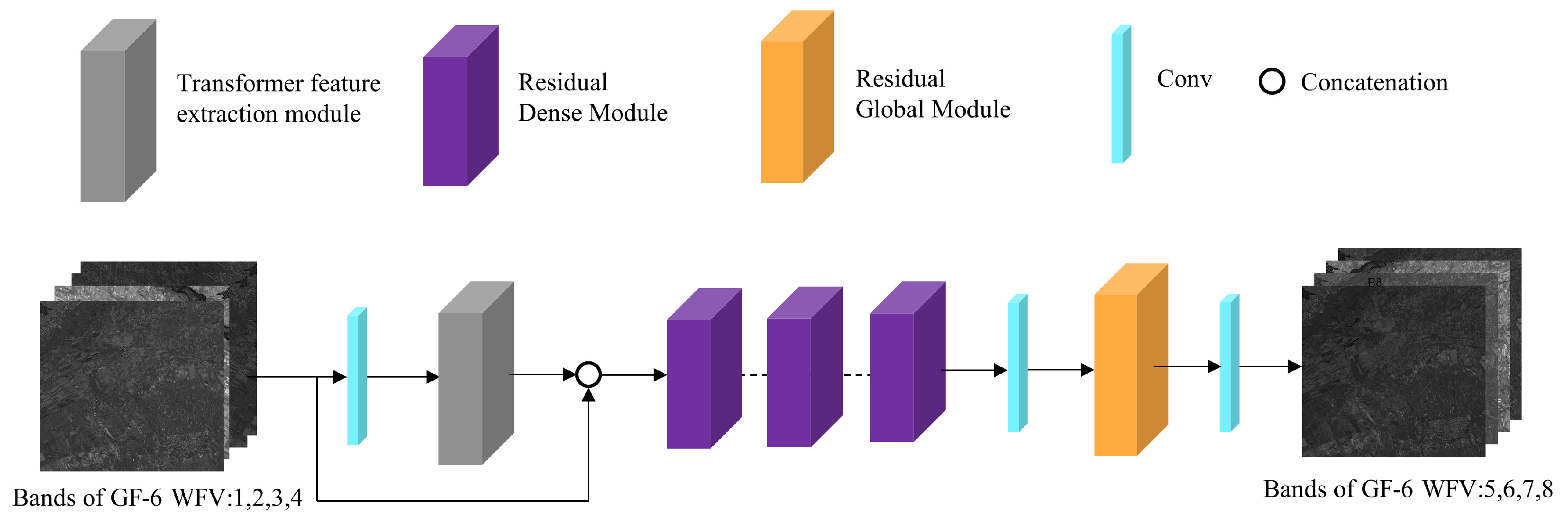
3.1. SRT Architecture
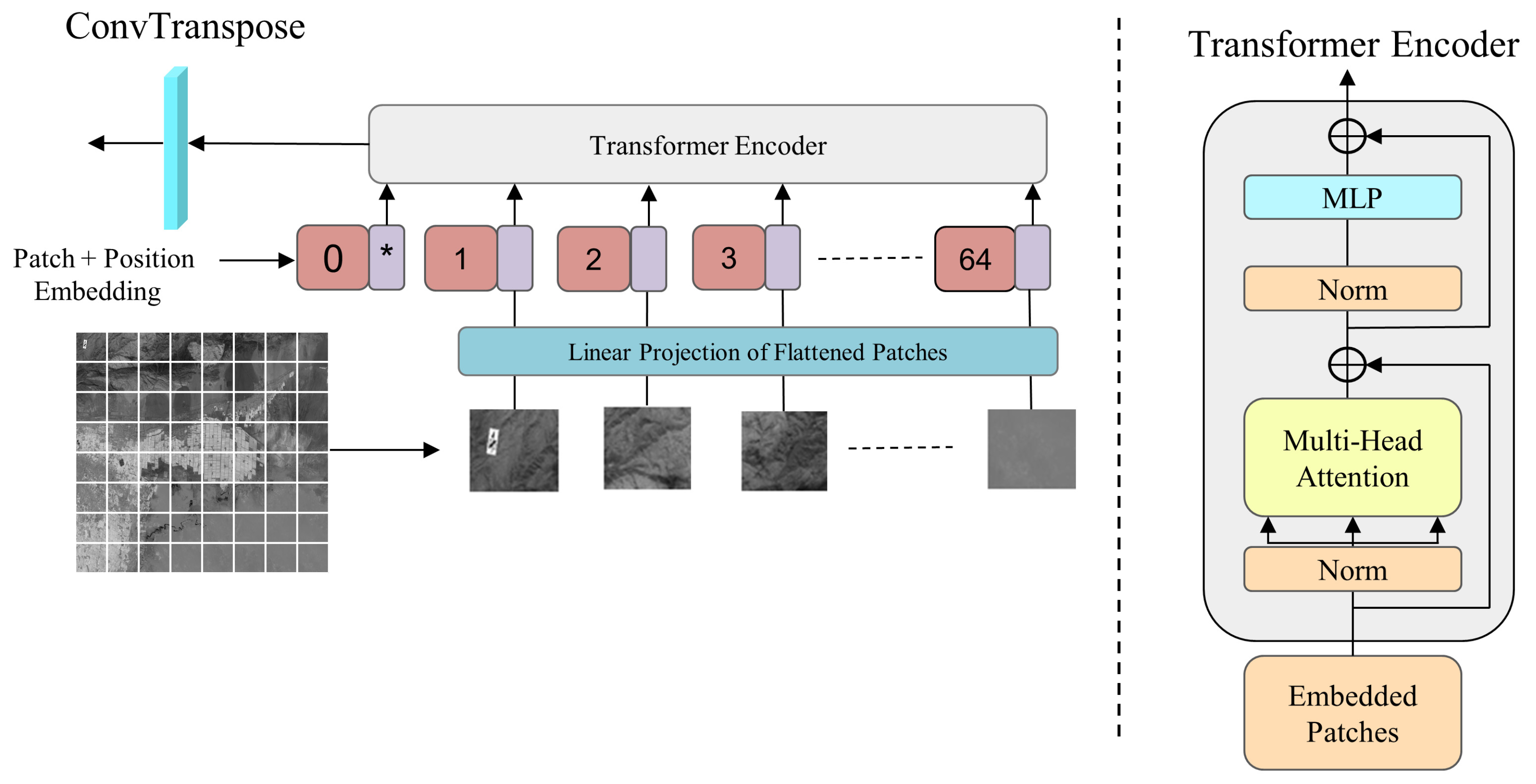
- The TFEM is used to extract correlation between spectra by self-attention mechanism.
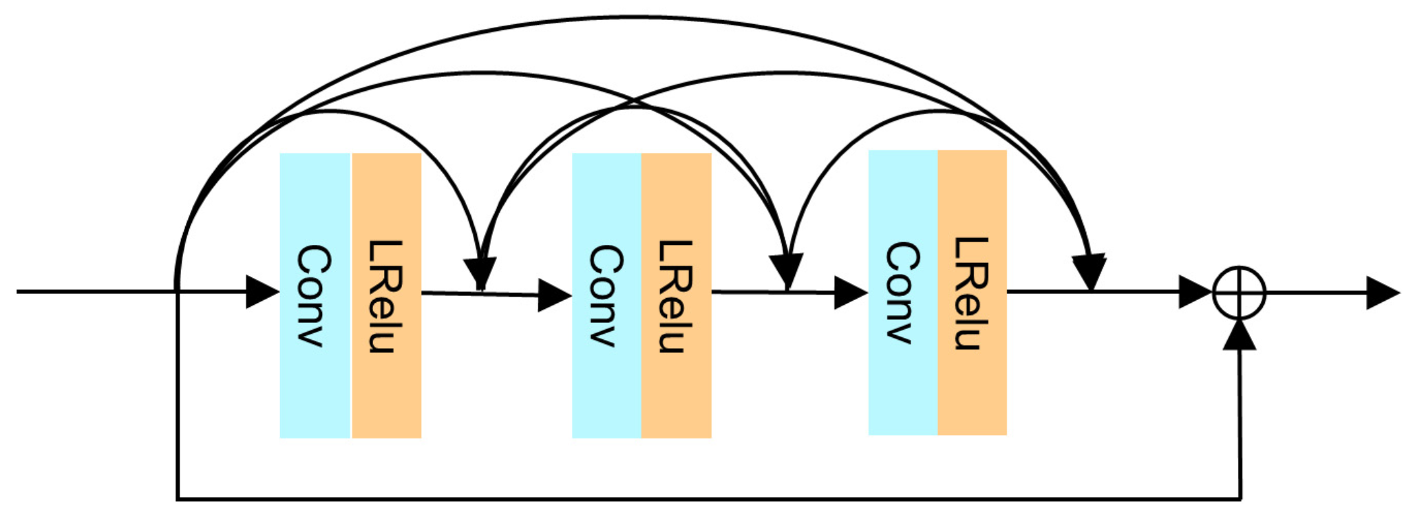
- The RDM, which can fully learn and reconstruct these local features to prevent gradient vanishing in training.
- The RGM is able to reconstruct these global features. Considering the model is ultimately used for GF-1 PMS (8 m) images, it doubles the spatial resolution compared to the trained GF-6 WFV (16 m) images. This module can prevent losing the texture details in the training or inference process.
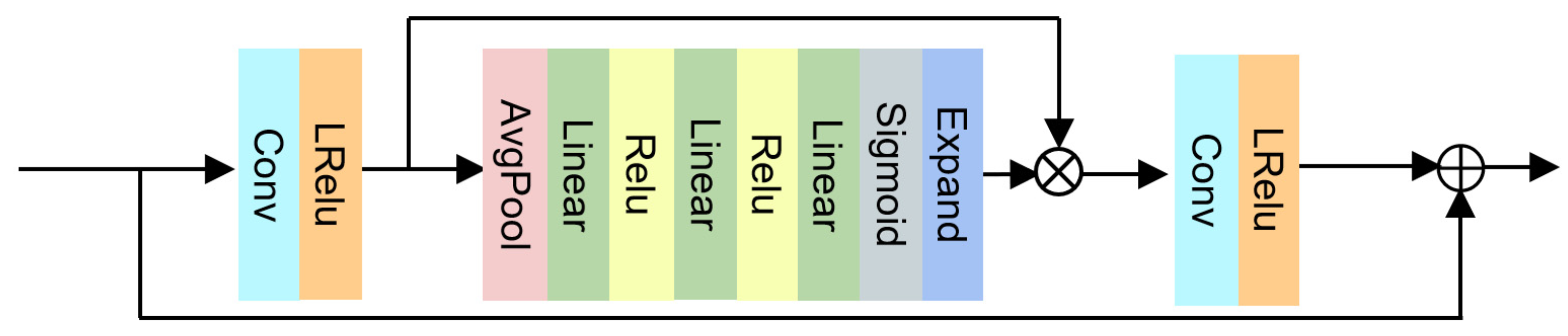
3.2. TFEM
3.3. RDM
3.4. RGM
3.5. Loss Function
3.6. Network Training and Parameter Settings
4. Experiments
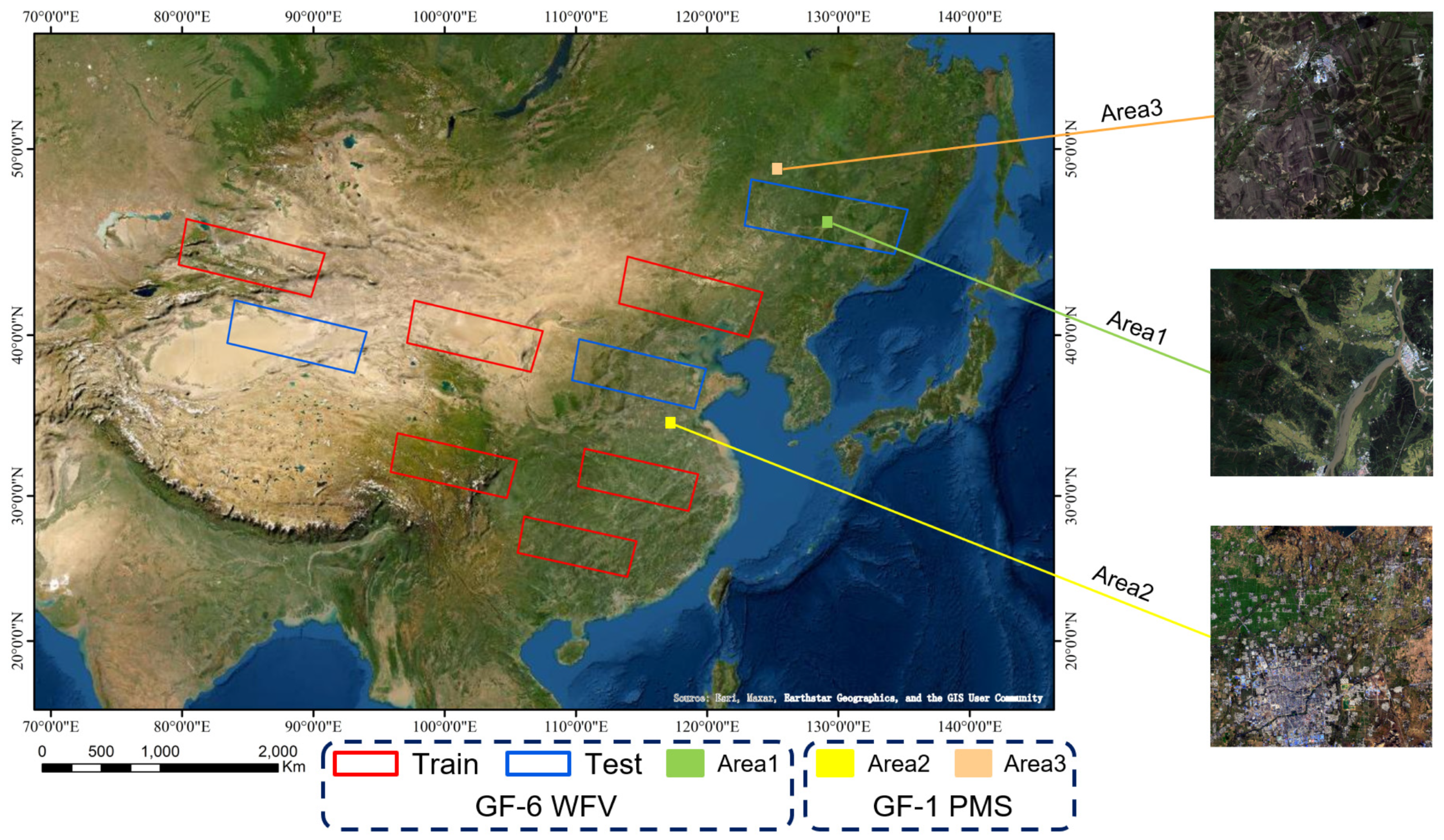
4.1. Dataset Description
4.2. Evaluation Metrics
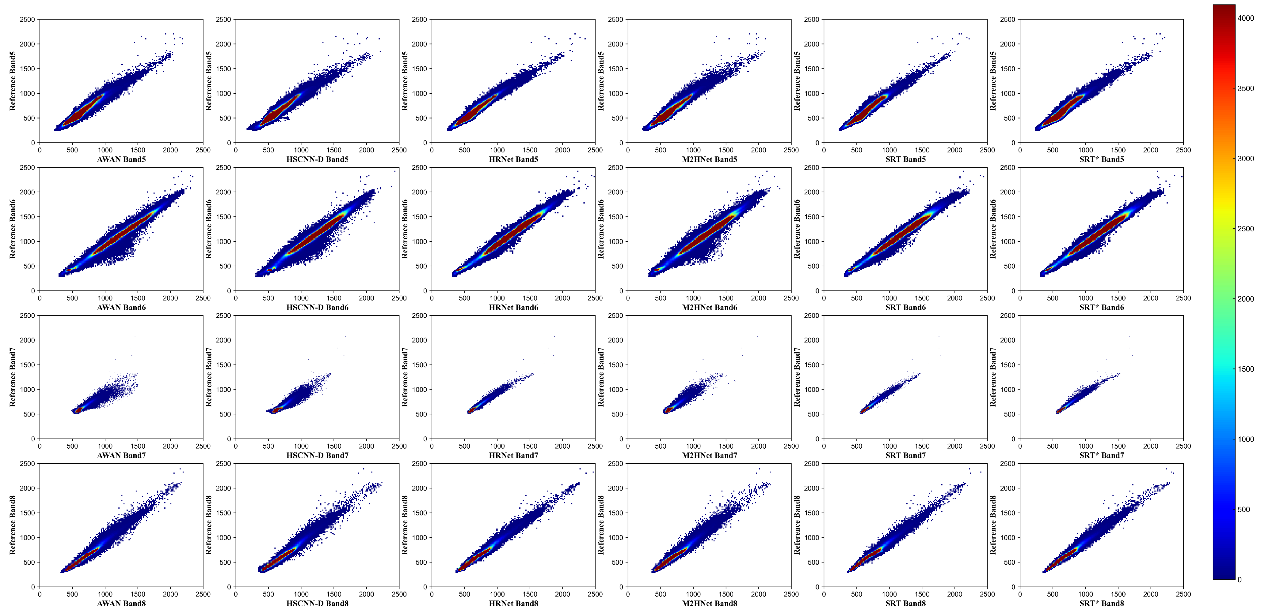
4.3. Similarity-Based Evaluation
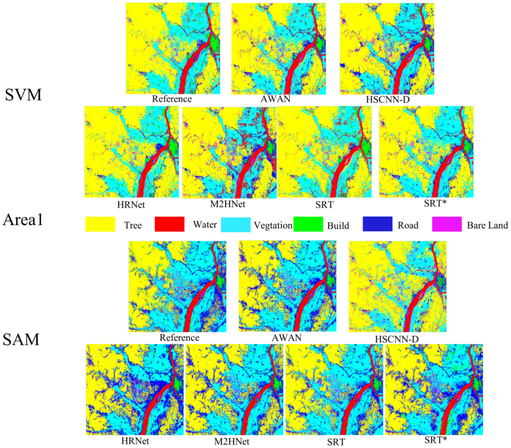
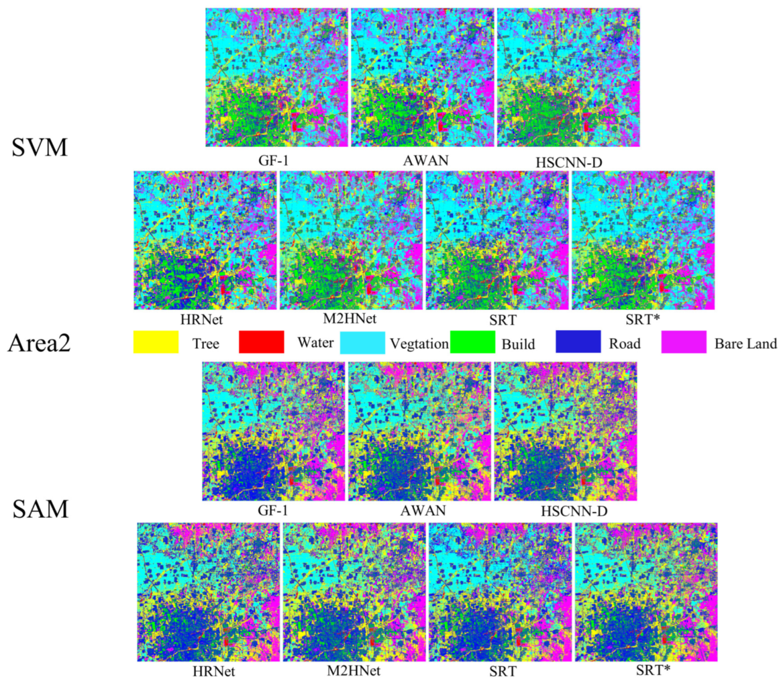
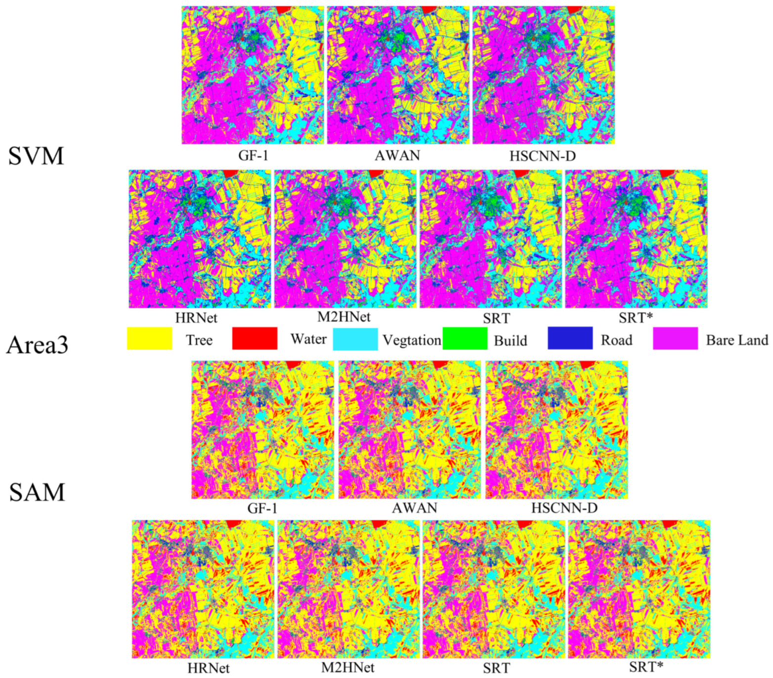
4.4. Classification-Based Evaluation
4.5. Comparison of Computational Cost
5. Conclusions
Author Contributions
Funding
Data Availability Statement
Acknowledgments
Conflicts of Interest
Appendix A

| Application | Satellite | Sensor | Acquisition Data | Location |
|---|---|---|---|---|
| Train | GF-6 | WFV | 10 October 2018 | 85.8E 44.6N |
| GF-6 | WFV | 4 September 2018 | 100.5E 31.3N | |
| GF-6 | WFV | 11 October 2018 | 102.5E 40.2N | |
| GF-6 | WFV | 5 October 2018 | 110.1E 26.9N | |
| GF-6 | WFV | 29 October 2018 | 114.8E 31.3N | |
| GF-6 | WFV | 18 September 2018 | 118.6E 42.4N | |
| Test | GF-6 | WFV | 1 October 2018 | 88.8E 40.2N |
| GF-6 | WFV | 17 October 2018 | 114.9E 38.0N | |
| GF-6 | WFV | 16 September 2018 | 129.9E 46.8N | |
| Area1 | GF-6 | WFV | 16 September 2018 | 129.9E 46.8N |
| Area2 | GF-1 | PMS1 | 4 November 2016 | 125.3E 48.8N |
| Area3 | GF-1 | PMS2 | 21 June 2018 | 117.2E 35.2N |
References
- Wu, Z.; Zhang, J.; Deng, F.; Zhang, S.; Zhang, D.; Xun, L.; Javed, T.; Liu, G.; Liu, D.; Ji, M. Fusion of GF and MODIS Data for Regional-Scale Grassland Community Classification with EVI2 Time-Series and Phenological Features. Remote Sens. 2021, 13, 835. [Google Scholar] [CrossRef]
- Jiang, X.; Fang, S.; Huang, X.; Liu, Y.; Guo, L. Rice Mapping and Growth Monitoring Based on Time Series GF-6 Images and Red-Edge Bands. Remote Sens. 2021, 13, 579. [Google Scholar] [CrossRef]
- Kang, Y.; Hu, X.; Meng, Q.; Zou, Y.; Zhang, L.; Liu, M.; Zhao, M. Land Cover and Crop Classification Based on Red Edge Indices Features of GF-6 WFV Time Series Data. Remote Sens. 2021, 13, 4522. [Google Scholar] [CrossRef]
- Arad, B.; Ben-Shahar, O. Sparse recovery of hyperspectral signal from natural RGB images. In Proceedings of the European Conference on Computer Vision, Amsterdam, The Netherlands, 11–14 October 2016; pp. 19–34. [Google Scholar]
- Aeschbacher, J.; Wu, J.; Timofte, R. In defense of shallow learned spectral reconstruction from RGB images. In Proceedings of the IEEE International Conference on Computer Vision Workshops, Venice, Italy, 22–29 October 2017; pp. 471–479. [Google Scholar]
- Fu, Y.; Zheng, Y.; Zhang, L.; Huang, H. Spectral Reflectance Recovery From a Single RGB Image. IEEE Trans. Comput. Imaging 2018, 4, 382–394. [Google Scholar] [CrossRef]
- Li, Y.; Wang, C.; Zhao, J. Locally Linear Embedded Sparse Coding for Spectral Reconstruction From RGB Images. IEEE Signal Process. Lett. 2018, 25, 363–367. [Google Scholar] [CrossRef]
- Geng, Y.; Mei, S.; Tian, J.; Zhang, Y.; Du, Q. Spatial Constrained Hyperspectral Reconstruction from RGB Inputs Using Dictionary Representation. In Proceedings of the IGARSS 2019–2019 IEEE International Geoscience and Remote Sensing Symposium, Yokohama, Japan, 28 July–2 August 2019; pp. 3169–3172. [Google Scholar] [CrossRef]
- Gao, L.; Hong, D.; Yao, J.; Zhang, B.; Gamba, P.; Chanussot, J. Spectral superresolution of multispectral imagery with joint sparse and low-rank learning. IEEE Trans. Geosci. Remote Sens. 2020, 59, 2269–2280. [Google Scholar] [CrossRef]
- Xiong, Z.; Shi, Z.; Li, H.; Wang, L.; Liu, D.; Wu, F. Hscnn: Cnn-based hyperspectral image recovery from spectrally undersampled projections. In Proceedings of the IEEE International Conference on Computer Vision Workshops, Venice, Italy, 22–29 October 2017; pp. 518–525. [Google Scholar]
- Alvarez-Gila, A.; Van De Weijer, J.; Garrote, E. Adversarial networks for spatial context-aware spectral image reconstruction from rgb. In Proceedings of the IEEE International Conference on Computer Vision Workshops, Venice, Italy, 22–29 October 2017; pp. 480–490. [Google Scholar]
- Koundinya, S.; Sharma, H.; Sharma, M.; Upadhyay, A.; Manekar, R.; Mukhopadhyay, R.; Karmakar, A.; Chaudhury, S. 2D-3D CNN based architectures for spectral reconstruction from RGB images. In Proceedings of the IEEE Conference on Computer Vision and Pattern Recognition Workshops, Salt Lake City, UT, USA, 18–23 June 2018; pp. 844–851. [Google Scholar]
- Shi, Z.; Chen, C.; Xiong, Z.; Liu, D.; Wu, F. Hscnn+: Advanced cnn-based hyperspectral recovery from rgb images. In Proceedings of the IEEE Conference on Computer Vision and Pattern Recognition Workshops, Salt Lake City, UT, USA, 18–23 June 2018; pp. 939–947. [Google Scholar]
- Zhao, Y.; Po, L.M.; Yan, Q.; Liu, W.; Lin, T. Hierarchical regression network for spectral reconstruction from RGB images. In Proceedings of the IEEE/CVF Conference on Computer Vision and Pattern Recognition Workshops, Seattle, WA, USA, 14–19 June 2020; pp. 422–423. [Google Scholar]
- Deng, L.; Sun, J.; Chen, Y.; Lu, H.; Duan, F.; Zhu, L.; Fan, T. M2H-Net: A Reconstruction Method For Hyperspectral Remotely Sensed Imagery. ISPRS J. Photogramm. Remote Sens. 2021, 173, 323–348. [Google Scholar] [CrossRef]
- Li, T.; Gu, Y. Progressive Spatial–Spectral Joint Network for Hyperspectral Image Reconstruction. IEEE Trans. Geosci. Remote Sens. 2021, 60, 1–14. [Google Scholar] [CrossRef]
- Zhang, X.; Xu, H. Reconstructing spectral reflectance by dividing spectral space and extending the principal components in principal component analysis. J. Opt. Soc. Am. A 2008, 25, 371–378. [Google Scholar] [CrossRef] [PubMed]
- Liu, X.; Liu, L. Improving chlorophyll fluorescence retrieval using reflectance reconstruction based on principal components analysis. IEEE Geosci. Remote Sens. Lett. 2015, 12, 1645–1649. [Google Scholar]
- Haneishi, H.; Hasegawa, T.; Hosoi, A.; Yokoyama, Y.; Tsumura, N.; Miyake, Y. System design for accurately estimating the spectral reflectance of art paintings. Appl. Opt. 2000, 39, 6621–6632. [Google Scholar] [CrossRef] [PubMed] [Green Version]
- Imai, F.H.; Berns, R.S. Spectral estimation using trichromatic digital cameras. In Proceedings of the International Symposium on Multispectral Imaging and Color Reproduction for Digital Archives, Chiba, Japan, 21–22 October 1999; Volume 42, pp. 1–8. [Google Scholar]
- Cheung, V.; Westland, S.; Li, C.; Hardeberg, J.; Connah, D. Characterization of trichromatic color cameras by using a new multispectral imaging technique. JOSA A 2005, 22, 1231–1240. [Google Scholar] [CrossRef] [PubMed]
- Zhang, J.; Su, R.; Ren, W.; Fu, Q.; Nie, Y. Learnable Reconstruction Methods from RGB Images to Hyperspectral Imaging: A Survey. arXiv 2021, arXiv:2106.15944. [Google Scholar]
- Arad, B.; Ben-Shahar, O.; Timofte, R.; Gool, L.V.; Yang, M.H. NTIRE 2018 Challenge on Spectral Reconstruction from RGB Images. In Proceedings of the 2018 IEEE/CVF Conference on Computer Vision and Pattern Recognition Workshops (CVPRW), Salt Lake City, UT, USA, 18–23 June 2018. [Google Scholar]
- Li, J.; Wu, C.; Song, R.; Li, Y.; Liu, F. Adaptive weighted attention network with camera spectral sensitivity prior for spectral reconstruction from RGB images. In Proceedings of the IEEE/CVF Conference on Computer Vision and Pattern Recognition Workshops, Seattle, WA, USA, 14–19 June 2020; pp. 462–463. [Google Scholar]
- Vaswani, A.; Shazeer, N.; Parmar, N.; Uszkoreit, J.; Jones, L.; Gomez, A.N.; Kaiser, Ł.; Polosukhin, I. Attention is all you need. In Proceedings of the Advances in Neural Information Processing Systems 30: Annual Conference on Neural Information Processing Systems 2017, Long Beach, CA, USA, 4–9 December 2017. [Google Scholar]
- Lin, T.; Wang, Y.; Liu, X.; Qiu, X. A survey of transformers. arXiv 2021, arXiv:2106.04554. [Google Scholar]
- Dosovitskiy, A.; Beyer, L.; Kolesnikov, A.; Weissenborn, D.; Zhai, X.; Unterthiner, T.; Dehghani, M.; Minderer, M.; Heigold, G.; Gelly, S.; et al. An image is worth 16x16 words: Transformers for image recognition at scale. arXiv 2020, arXiv:2010.11929. [Google Scholar]
- Touvron, H.; Cord, M.; Douze, M.; Massa, F.; Sablayrolles, A.; Jégou, H. Training data-efficient image transformers & distillation through attention. In Proceedings of the International Conference on Machine Learning (PMLR), Virtual Event, 13–14 August 2021; pp. 10347–10357. [Google Scholar]
- Carion, N.; Massa, F.; Synnaeve, G.; Usunier, N.; Kirillov, A.; Zagoruyko, S. End-to-end object detection with transformers. In Proceedings of the European Conference on Computer Vision, Seattle, WA, USA, 14–19 June 2020; pp. 213–229. [Google Scholar]
- Zhu, X.; Su, W.; Lu, L.; Li, B.; Wang, X.; Dai, J. Deformable detr: Deformable transformers for end-to-end object detection. arXiv 2020, arXiv:2010.04159. [Google Scholar]
- Zheng, S.; Lu, J.; Zhao, H.; Zhu, X.; Luo, Z.; Wang, Y.; Fu, Y.; Feng, J.; Xiang, T.; Torr, P.H.; et al. Rethinking semantic segmentation from a sequence-to-sequence perspective with transformers. In Proceedings of the IEEE/CVF Conference on Computer Vision and Pattern Recognition, Nashville, TN, USA, 20–25 June 2021; pp. 6881–6890. [Google Scholar]
- Valanarasu, J.M.J.; Oza, P.; Hacihaliloglu, I.; Patel, V.M. Medical transformer: Gated axial-attention for medical image segmentation. In Proceedings of the International Conference on Medical Image Computing and Computer-Assisted Intervention, Strasbourg, France, 27 September–1 October 2021; pp. 36–46. [Google Scholar]
- Arad Hudson, D.; Zitnick, L. Compositional Transformers for Scene Generation. In Proceedings of the 34th Conference on Neural Information Processing Systems (NeurIPS 2020), Online, 6–12 December 2020; pp. 9506–9520. [Google Scholar]
- He, K.; Chen, X.; Xie, S.; Li, Y.; Dollár, P.; Girshick, R. Masked autoencoders are scalable vision learners. arXiv 2021, arXiv:2111.06377. [Google Scholar]
- He, K.; Zhang, X.; Ren, S.; Sun, J. Deep residual learning for image recognition. In Proceedings of the IEEE Conference on Computer Vision and Pattern Recognition, Las Vegas, NV, USA, 27–30 June 2016; pp. 770–778. [Google Scholar]
- Huang, G.; Liu, Z.; Van Der Maaten, L.; Weinberger, K.Q. Densely connected convolutional networks. In Proceedings of the IEEE Conference on Computer Vision and Pattern Recognition, Venice, Italy, 22–29 October 2017; pp. 4700–4708. [Google Scholar]
- LeCun, Y.; Boser, B.; Denker, J.; Henderson, D.; Howard, R.; Hubbard, W.; Jackel, L. Handwritten digit recognition with a back-propagation network. In Proceedings of the Advances in Neural Information Processing Systems 2, Denver, CO, USA, 27–30 November 1989. [Google Scholar]
- Hu, J.; Shen, L.; Sun, G. Squeeze-and-excitation networks. In Proceedings of the IEEE Conference on Computer Vision and Pattern Recognition, Salt Lake City, UT, USA, 18–23 June 2018; pp. 7132–7141. [Google Scholar]
- Huynh-Thu, Q.; Ghanbari, M. Scope of validity of PSNR in image/video quality assessment. Electron. Lett. 2008, 44, 800–801. [Google Scholar] [CrossRef]
- CRESDA. China Centre For Resources Satellite Data and Application. 2021. Available online: http://www.cresda.com/CN/index.shtml (accessed on 2 June 2022).
- Yuhas, R.H.; Goetz, A.F.; Boardman, J.W. Discrimination among semi-arid landscape endmembers using the spectral angle mapper (SAM) algorithm. In Summaries of the Third Annual JPL Airborne Geoscience Workshop. Volume 1: AVIRIS Workshop; Jet Propulsion Laboratory: La Cañada Flintridge, CA, USA, 1992. [Google Scholar]
- Wang, Z.; Bovik, A.C.; Sheikh, H.R.; Simoncelli, E.P. Image quality assessment: From error visibility to structural similarity. IEEE Trans. Image Process. 2004, 13, 600–612. [Google Scholar] [CrossRef] [PubMed] [Green Version]


| GF-1 PMS | GF-6 WFV | ||||
|---|---|---|---|---|---|
| Band | Wavelength (nm) | Spatial Resolution (m) | Band | Wavelength (nm) | Spatial Resolution (m) |
| Blue | 450∼520 | 8 | Blue | 450∼520 | 16 |
| Green | 520∼590 | 8 | Green | 520∼590 | 16 |
| Red | 630∼690 | 8 | Red | 630∼690 | 16 |
| Nir | 730∼890 | 8 | Nir | 730∼890 | 16 |
| Red edge 1 | 690∼730 | 16 | |||
| Red edge 1 | 730∼770 | 16 | |||
| Purple | 400∼450 | 16 | |||
| Yellow | 590∼640 | 16 | |||
| Pan | 450∼900 | 2 | |||
| Parameter Name | Parameter Setting |
|---|---|
| Batch size Initial learning rate | 32 0.01 |
| Optimizer | Adam |
| Decay rate | 0.1 |
| Learning rate decay steps | 2000 steps |
| Epochs | 200 |
| Activation function | Relu Sigmod Leaky-Relu |
| Area1 | Area2 | Area3 | ||||
|---|---|---|---|---|---|---|
| Train | Test | Train | Test | Train | Test | |
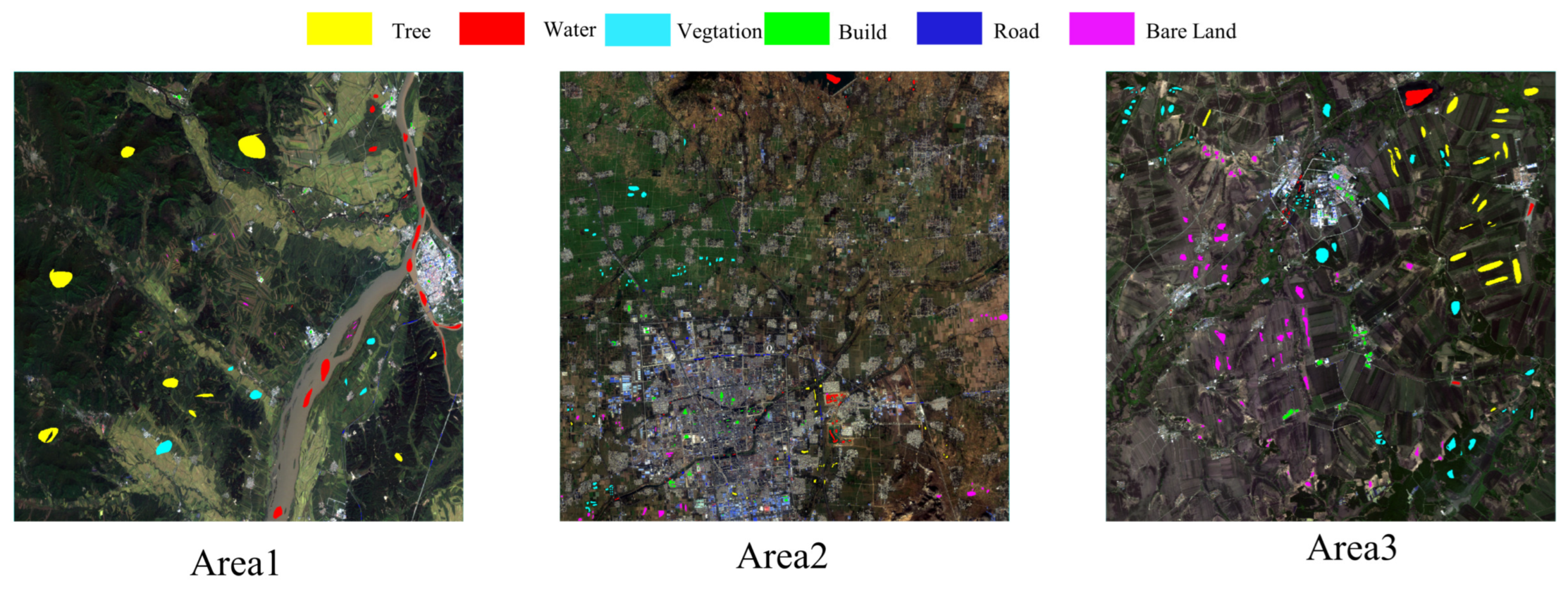
| Water | 6381 | 2451 | 3992 | 2661 | 1921 | 3487 |
| Build | 738 | 392 | 3008 | 2005 | 1219 | 1598 |
| Bare land | 101 | 99 | 4306 | 2870 | 1397 | 1491 |
| Plant | 2431 | 1273 | 4169 | 2780 | 7204 | 8551 |
| Tree | 10371 | 8361 | 1691 | 1127 | 6518 | 3131 |
| Road | 87 | 146 | 1592 | 1062 | 300 | 259 |
| Evaluation | Band | Method | |||||
|---|---|---|---|---|---|---|---|
| AWAN | HSCNN-D | HRNet | M2Hnet | SRT | SRT* | ||
| PSNR | band5 | 40.06 | 40.10 | 43.92 | 40.80 | 45.23 | 44.91 |
| band6 | 39.37 | 39.47 | 43.00 | 38.92 | 44.00 | 43.39 | |
| band7 | 42.51 | 41.71 | 46.56 | 42.50 | 48.29 | 47.81 | |
| band8 | 41.23 | 42.10 | 44.71 | 40.95 | 45.87 | 45.63 | |
| avg | 40.79 | 40.85 | 44.55 | 40.79 | 45.85 | 45.43 | |
| SSIM | band5 | 0.980 | 0.972 | 0.991 | 0.979 | 0.991 | 0.991 |
| band6 | 0.970 | 0.983 | 0.992 | 0.976 | 0.991 | 0.990 | |
| band7 | 0.980 | 0.985 | 0.990 | 0.973 | 0.992 | 0.992 | |
| band8 | 0.970 | 0.981 | 0.990 | 0.978 | 0.992 | 0.992 | |
| avg | 0.975 | 0.980 | 0.991 | 0.976 | 0.992 | 0.991 | |
| MRAE | band5 | 0.038 | 0.041 | 0.024 | 0.038 | 0.021 | 0.024 |
| band6 | 0.026 | 0.024 | 0.019 | 0.037 | 0.020 | 0.020 | |
| band7 | 0.031 | 0.032 | 0.022 | 0.036 | 0.019 | 0.025 | |
| band8 | 0.032 | 0.029 | 0.021 | 0.038 | 0.020 | 0.022 | |
| avg | 0.032 | 0.032 | 0.022 | 0.037 | 0.020 | 0.023 | |
| SAM | band5 | 1.66 | 1.59 | 1.17 | 1.68 | 1.06 | 1.07 |
| band6 | 1.21 | 1.23 | 0.87 | 1.36 | 0.81 | 0.84 | |
| band7 | 1.42 | 1.43 | 0.88 | 1.51 | 0.80 | 0.81 | |
| band8 | 1.66 | 1.50 | 1.08 | 1.72 | 1.00 | 1.02 | |
| avg | 1.49 | 1.44 | 1.00 | 1.57 | 0.92 | 0.93 | |
| RMSE | band5 | 0.010 | 0.012 | 0.008 | 0.016 | 0.007 | 0.010 |
| band6 | 0.015 | 0.021 | 0.007 | 0.011 | 0.009 | 0.014 | |
| band7 | 0.009 | 0.014 | 0.009 | 0.004 | 0.006 | 0.008 | |
| band8 | 0.010 | 0.013 | 0.007 | 0.016 | 0.007 | 0.010 | |
| avg | 0.011 | 0.015 | 0.008 | 0.012 | 0.008 | 0.011 | |
| SVM | AWAN | HSCNN-D | HRNet | M2HNet | SRT | SRT* | GF-6 |
|---|---|---|---|---|---|---|---|
| OA | 0.8909 | 0.9015 | 0.9030 | 0.9038 | 0.9237 | 0.9118 | 0.9291 |
| Kappa | 0.7900 | 0.8071 | 0.8106 | 0.8133 | 0.8321 | 0.8215 | 0.8357 |
| Water | 0.9560 | 0.8272 | 0.9733 | 0.9786 | 0.8324 | 0.9813 | 0.9847 |
| Build | 0.9217 | 0.8918 | 0.9849 | 0.9295 | 0.9777 | 0.9894 | 0.9817 |
| Bare Land | 0.5719 | 0.7455 | 0.5855 | 0.5804 | 0.5035 | 0.6646 | 0.6654 |
| Vegetation | 0.8803 | 0.8836 | 0.8836 | 0.8506 | 0.9140 | 0.8871 | 0.9262 |
| Tree | 0.8812 | 0.8196 | 0.8909 | 0.8983 | 0.8657 | 0.9001 | 0.9200 |
| Road | 0.5756 | 0.5857 | 0.5823 | 0.5785 | 0.4357 | 0.5872 | 0.5768 |
| SAM | AWAN | HSCNN-D | HRNet | M2HNet | SRT | SRT* | GF-6 |
|---|---|---|---|---|---|---|---|
| OA | 0.8743 | 0.8709 | 0.8782 | 0.8701 | 0.8939 | 0.8854 | 0.8992 |
| Kappa | 0.7435 | 0.7409 | 0.7513 | 0.7401 | 0.8012 | 0.7821 | 0.8036 |
| Water | 0.8970 | 0.8683 | 0.8324 | 0.8498 | 0.8823 | 0.8849 | 0.8500 |
| Build | 0.5148 | 0.6386 | 0.5077 | 0.5339 | 0.4636 | 0.4851 | 0.4715 |
| Bare Land | 0.7121 | 0.7490 | 0.5035 | 0.6606 | 0.5539 | 0.5746 | 0.8823 |
| Vegetation | 0.9518 | 0.9429 | 0.914 | 0.9492 | 0.9202 | 0.9411 | 0.9278 |
| Tree | 0.8799 | 0.8774 | 0.9157 | 0.8862 | 0.9258 | 0.9028 | 0.9331 |
| Road | 0.5703 | 0.6183 | 0.4357 | 0.6449 | 0.4196 | 0.6977 | 0.6976 |
| SVM | AWAN | HSCNN-D | HRNet | M2Hnet | SRT | SRT* | GF-1 |
|---|---|---|---|---|---|---|---|
| OA | 0.8662 | 0.8749 | 0.8839 | 0.8788 | 0.8862 | 0.8853 | 0.8648 |
| Kappa | 0.8309 | 0.8359 | 0.8507 | 0.8399 | 0.8655 | 0.8548 | 0.8223 |
| Water | 0.9754 | 0.9808 | 0.9854 | 0.9880 | 0.9881 | 0.9844 | 0.9775 |
| Build | 0.7527 | 0.7638 | 0.8299 | 0.8045 | 0.7590 | 0.7514 | 0.7519 |
| Bare Land | 0.8378 | 0.8879 | 0.8492 | 0.8600 | 0.9398 | 0.9395 | 0.8527 |
| Vegetation | 0.9614 | 0.9505 | 0.9535 | 0.9555 | 0.9543 | 0.9573 | 0.9531 |
| Tree | 0.8279 | 0.7876 | 0.8358 | 0.8227 | 0.7940 | 0.7907 | 0.8370 |
| Road | 0.6650 | 0.6784 | 0.6947 | 0.6547 | 0.6458 | 0.6558 | 0.6264 |
| SVM | AWAN | HSCNN-D | HRNet | M2Hnet | SRT | SRT* | GF-1 |
|---|---|---|---|---|---|---|---|
| OA | 0.8046 | 0.7954 | 0.8047 | 0.8058 | 0.8196 | 0.8066 | 0.7923 |
| Kappa | 0.7920 | 0.7836 | 0.7921 | 0.7947 | 0.8048 | 0.7956 | 0.7822 |
| Water | 0.9973 | 0.9972 | 0.9907 | 0.9972 | 0.9997 | 0.9990 | 0.9988 |
| Build | 0.9087 | 0.9104 | 0.9087 | 0.9381 | 0.8822 | 0.9140 | 0.9015 |
| Bare Land | 0.4623 | 0.4403 | 0.4625 | 0.4288 | 0.4812 | 0.4611 | 0.4233 |
| Vegetation | 0.8059 | 0.7872 | 0.8059 | 0.7959 | 0.8418 | 0.8062 | 0.7775 |
| Tree | 0.8610 | 0.8726 | 0.8610 | 0.9264 | 0.9429 | 0.8737 | 0.9160 |
| Road | 0.9874 | 0.9886 | 0.9874 | 0.9875 | 0.9779 | 0.9852 | 0.9776 |
| SVM | AWAN | HSCNN-D | HRNet | M2Hnet | SRT | SRT* | GF-1 |
|---|---|---|---|---|---|---|---|
| OA | 0.9303 | 0.9212 | 0.9327 | 0.9322 | 0.9487 | 0.9406 | 0.9246 |
| Kappa | 0.9258 | 0.9127 | 0.9302 | 0.9190 | 0.9357 | 0.9348 | 0.9157 |
| Water | 0.991 | 0.9854 | 0.9897 | 0.9888 | 0.9880 | 0.9853 | 0.9931 |
| Build | 0.6304 | 0.6299 | 0.5710 | 0.5933 | 0.6650 | 0.5944 | 0.4950 |
| Bare Land | 0.9047 | 0.9347 | 0.9545 | 0.9564 | 0.9248 | 0.9525 | 0.9149 |
| Vegetation | 0.9571 | 0.9358 | 0.9624 | 0.9608 | 0.9798 | 0.9725 | 0.9691 |
| Tree | 0.9520 | 0.9492 | 0.9598 | 0.9503 | 0.9728 | 0.9725 | 0.9472 |
| Road | 0.9620 | 0.9535 | 0.9638 | 0.9613 | 0.9894 | 0.9682 | 0.9660 |
| SVM | AWAN | HSCNN-D | HRNet | M2Hnet | SRT | SRT* | GF-1 |
|---|---|---|---|---|---|---|---|
| OA | 0.8298 | 0.8344 | 0.8439 | 0.8301 | 0.8490 | 0.8438 | 0.8367 |
| Kappa | 0.7397 | 0.7445 | 0.7563 | 0.7420 | 0.7599 | 0.7509 | 0.7484 |
| Water | 0.8583 | 0.8583 | 0.8714 | 0.8485 | 0.8856 | 0.8892 | 0.8574 |
| Build | 0.3822 | 0.4195 | 0.4016 | 0.4119 | 0.4345 | 0.4338 | 0.3973 |
| Bare Land | 0.8599 | 0.8617 | 0.8804 | 0.8596 | 0.8800 | 0.8779 | 0.877 |
| Vegetation | 0.6271 | 0.6101 | 0.6786 | 0.6732 | 0.6758 | 0.6205 | 0.6083 |
| Tree | 0.9309 | 0.9289 | 0.9396 | 0.9237 | 0.9375 | 0.9276 | 0.9363 |
| Road | 0.6356 | 0.6634 | 0.6574 | 0.6634 | 0.6647 | 0.6634 | 0.6436 |
| AWAN | HSCNN-D | HRNet | M2Hnet | SRT | SRT* | |
|---|---|---|---|---|---|---|
| Params (M) | 21.58 | 4.62 | 32.04 | 22.73 | 17.62 | 17.54 |
| GFLOPs | 352.85 | 75.64 | 40.89 | 245.86 | 121.66 | 120.45 |
| Time (S) | 0.21 | 1.21 | 0.41 | 0.24 | 0.27 | 0.25 |
Publisher’s Note: MDPI stays neutral with regard to jurisdictional claims in published maps and institutional affiliations. |
© 2022 by the authors. Licensee MDPI, Basel, Switzerland. This article is an open access article distributed under the terms and conditions of the Creative Commons Attribution (CC BY) license (https://creativecommons.org/licenses/by/4.0/).
Share and Cite
Mu, K.; Zhang, Z.; Qian, Y.; Liu, S.; Sun, M.; Qi, R. SRT: A Spectral Reconstruction Network for GF-1 PMS Data Based on Transformer and ResNet. Remote Sens. 2022, 14, 3163. https://doi.org/10.3390/rs14133163
Mu K, Zhang Z, Qian Y, Liu S, Sun M, Qi R. SRT: A Spectral Reconstruction Network for GF-1 PMS Data Based on Transformer and ResNet. Remote Sensing. 2022; 14(13):3163. https://doi.org/10.3390/rs14133163
Chicago/Turabian StyleMu, Kai, Ziyuan Zhang, Yurong Qian, Suhong Liu, Mengting Sun, and Ranran Qi. 2022. "SRT: A Spectral Reconstruction Network for GF-1 PMS Data Based on Transformer and ResNet" Remote Sensing 14, no. 13: 3163. https://doi.org/10.3390/rs14133163
APA StyleMu, K., Zhang, Z., Qian, Y., Liu, S., Sun, M., & Qi, R. (2022). SRT: A Spectral Reconstruction Network for GF-1 PMS Data Based on Transformer and ResNet. Remote Sensing, 14(13), 3163. https://doi.org/10.3390/rs14133163