Article

Improving the Accuracy of Groundwater Storage Estimates Based on Groundwater Weighted Fusion Model

1
School of Surveying and Land Information Engineering, Henan Polytechnic University, Jiaozuo 454000, China
2
Qian Xuesen Laboratory of Technology, China Academy of Space Technology, Beijing 100094, China
3
School of Geomatics, Liaoning Technical University, Fuxin 123000, China
4
School of Electronics and Information Engineering, Harbin Institute of Technology, Harbin 150001, China
5
College of Water Sciences, Beijing Normal University, Beijing 100875, China
*
Author to whom correspondence should be addressed.
These authors contributed equally to this work.
Remote Sens. 2022, 14(1), 202; https://doi.org/10.3390/rs14010202
Submission received: 27 October 2021 / Revised: 15 December 2021 / Accepted: 17 December 2021 / Published: 2 January 2022
(This article belongs to the Topic Water Management in the Era of Climatic Change)

Abstract

:
It is an effective measure to estimate groundwater storage anomalies (GWSA) by combining Gravity Recovery and Climate Experiment (GRACE) data and hydrological models. However, GWSA results based on a single hydrological model and GRACE data may have greater uncertainties, and it is difficult to verify in some regions where in situ groundwater-level measurements are limited. First, to solve this problem, a groundwater weighted fusion model (GWFM) is presented, based on the extended triple collocation (ETC) method. Second, the Shiyang River Basin (SYRB) is taken as an example, and in situ groundwater-level measurements are used to evaluate the performance of the GWFM. The comparison indicates that the correlation coefficient (CC) and Nash-Sutcliffe efficiency coefficient (NSE) are increased by 9–40% and 23–657%, respectively, relative to the original results. Moreover, the root mean squared error (RMSE) is reduced by 9–28%, which verifies the superiority of the GWFM. Third, the spatiotemporal distribution and influencing factors of GWSA in the Hexi Corridor (HC) are comprehensively analyzed during the period between 2003 and 2016. The results show that GWSA decline, with a trend of −2.37 ± 0.38 mm/yr from 2003 to 2010, and the downward trend after 2011 (−0.46 ± 1.35 mm/yr) slow down significantly compared to 2003–2010. The spatial distribution obtained by the GWFM is more reliable compared to the arithmetic average results, and GWFM-based GWSA fully retain the advantages of different models, especially in the southeastern part of the SYRB. Additionally, a simple index is used to evaluate the contributions of climatic factors and human factors to groundwater storage (GWS) in the HC and its different subregions. The index indicates that climate factors occupy a dominant position in the SLRB and SYRB, while human factors have a significant impact on GWS in the Heihe River Basin (HRB). This study can provide suggestions for the management and assessments of groundwater resources in some arid regions.

1. Introduction

As an important component of terrestrial water storage (TWS), groundwater plays a key role in domestic, agriculture and industrial use, as well as ecosystems [1,2]. More than 38% of the world’s population lives in arid or semi-arid zones [3], where groundwater is usually the dominant freshwater resource, supplying domestic use and irrigation water [4]. Especially in northwest China, groundwater resources have been facing the risk of depletion, which may lead to the ecological environment of the region losing its ability to self-repair and endangering local ecological security [5]. Therefore, accurate estimation of groundwater storage anomalies (GWSA) is essential for the effective use of local groundwater resources. The traditional method of monitoring groundwater level mainly uses monitoring wells. However, monitoring wells are scarce, and the observation records are short and discontinuous, restricting research related to GWSA [2,6,7]. Therefore, it is important to seek an alternative method to obtain ground-based network data for monitoring of large-scale groundwater storage (GWS) variations.
Since March 2002, Gravity Recovery and Climate Experiment (GRACE) satellites have provided an opportunity to assess global TWS changes, with a resolution of ~300 km [8,9,10]. Currently, the GRACE gravity satellites are the only way to sense water storage at all levels, including soil moisture (SM), snow-water equivalent (SWE), canopy water storage (CWS), and GWS [10]. To isolate the GWS component from TWS, water storage changes of other components have to be estimated based on hydrological models [11,12]. At present, there are several frequently employed hydrological models and reanalysis datasets, such as the Global Land Data Assimilation System (GLDAS) [13], the WaterGAP Global Hydrology model (WGHM) [14], and the ERA5 reanalysis dataset [15,16]. Furthermore, previous studies have demonstrated the effectiveness of GRACE observations to estimate GWSA in many typically regions of the world, e.g., the Central Valley of California [17,18], northwest India [9,19,20], and the North China Plain [1,21,22].
Currently, most studies mainly rely on a single hydrological model to separate GWS components from GRACE-derived TWS [23,24,25]. However, the accuracy of these models is restricted by uncertainties in climate forcing (particularly precipitation), model parameters, and deficiencies in model structure [26,27,28,29,30,31]. Therefore, the effective combination of multiple models can improve the performance of hydrological simulations relative to a single model. For instance, Shamseldin et al. [32] used the method of multi-model ensemble to develop more skillful and reliable probabilistic hydrologic prediction. The results confirmed that better estimates of water storage can be obtained by combining the model outputs of different hydrological models. Long et al. [33] used the Bayesian model-averaging technique, which can merge multiple TWS products to analyze the spatiotemporal variability of TWS. Mehrnegar [27] presented the dynamic model-data-averaging method, which can be used to merge multiple TWS simulations. The result indicated that linear trends and seasonality within global hydrological models can be improved by using the dynamic model-data-averaging method. These multi-model techniques prove to provide accurate estimates by combining different models according to the different weighting strategies [32,34].
Triple collocation (TC) is a statistical method to estimate the random-error variance of three independent datasets [35]. Currently, the TC method has been used to estimate measurement errors of GRACE data [36]. Specifically, Khaki et al. [37] and Nigatu et al. [38] estimated the changes in key water-storage components by using the GRACE data and soil-moisture data based on the TC analysis method. Yin and Park [39] proposed a simple least-square merging approach using error characteristics quantified from the TC approach to estimate weight. Compared to the classic TC approach, the extended triple collocation (ETC), proposed by McColl [40], can obtain an additional evaluation index, that is, the correlation coefficient relative to the unknown true value. Up to now, there are few studies that have merged datasets from different sources based on the ETC method.
The Hexi Corridor (HC) is one of the most agriculturally rich areas of northwest China, which is characterized as an irrigation district of “no irrigation, no agriculture” [5,41]. Moreover, groundwater resources have been depleted on a large scale in the area due to poor management of groundwater exploitation [42]. The policy of building a water-saving society was introduced in Zhangye City of Gansu Province in 2001 [43]. The government initiated a policy called the Key Governance Planning Project of the Shiyang River Basin in 2007, which aimed to improve the ecological conditions of the area [44,45]. Accurate estimation of GWS is essential for understanding the complex hydrological process and formulating sustainable management policies for groundwater resources in the region.
The purpose of this study is to improve the accuracy of groundwater storage estimates in some regions where in situ groundwater-level measurements are limited and to quantify the impact of climate change and human activities. Specifically, a weighted fusion model is proposed, based on the squared correlation coefficient and error variance calculated by the ETC [40,46] method. The ratio of these two indicators is used to develop the groundwater weighted fusion model (GWFM), which is helpful in merging GWSA based on the GRACE and multiple hydrological models, and compare it with the original results. In addition, a simple and effective method is used to evaluate the contribution of climate factors and human factors to GWS.

2. Materials and Methods
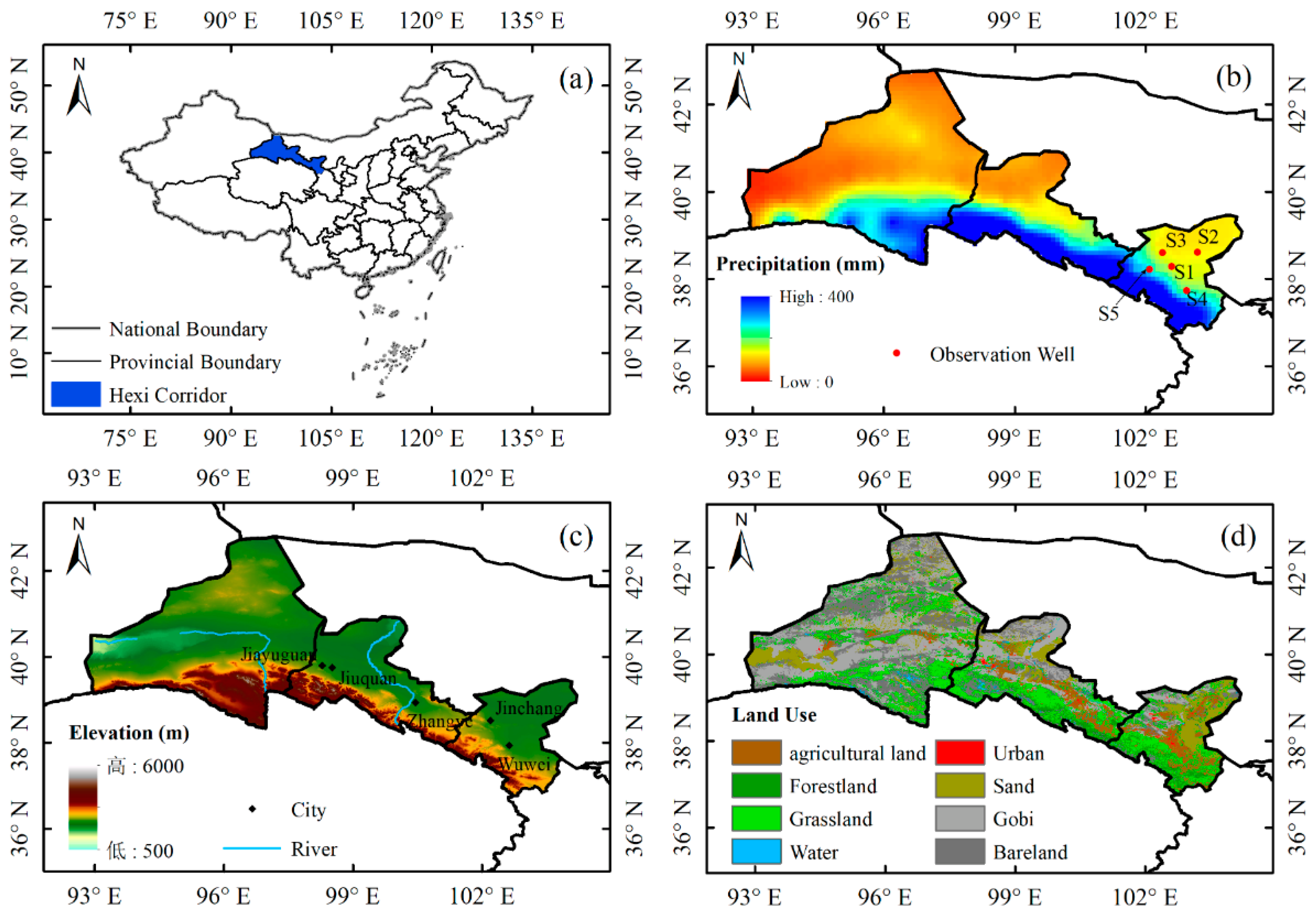
2.1. Study Area

The HC is located in Northwest China (92°12′–104°20′ E, 37°17′–42°48′ N) (Figure 1a), including the five prefecture-level cities of Wuwei, Jinchang, Zhangye, Jiuquan, and Jiayuguan (Figure 1c, http://srtm.csi.cgiar.org (accessed on 10 August 2021)) [47]. The three major rivers of the HC, from west to east, are the Shule River, the Heihe River and the Shiyang River, originating from the Qilian Mountains. The HC is mainly covered by bare land and gobi, and agricultural land is concentrated in the Shiyang River Basin (SYRB) and Heihe River Basin (HRB) (Figure 1d, https://www.resdc.cn (accessed on 10 August 2021)) [48]. It belongs to the arid continental climate, with an average annual temperature ranging from 8 to 10 °C [42], and the annual evaporation is 1500–3200 mm [49]. The rainfall shows a decreasing trend from east to west (Figure 1b, http://data.cma.cn (accessed on 10 August 2021)), and ~80% of rainfall occurs during July–August [50]. The Qilian Mountains in the south nurture extensive glaciers and snow, which is an important freshwater resource for downstream cities critical to easing agricultural drought and other human activities in the HC [51].

2.2. Materials

2.2.1. GRACE Data

The GRACE RL05 Mascon solutions are utilized to derive TWS anomalies in this study, which are provided by the Center for Space Research (CSR) [52]. Monthly TWS anomalies are provided from April 2002 to June 2017, with a spatial resolution of 0.5 × 0.5°. The regularization constraint on mascon solutions is derived from original GRACE information with no empirical filtering post-processing [52,53]. Therefore, the product can capture all the signals observed by GRACE within the measurement noise level and be used without further processing [54]. Missing data in the CSR Mascon are filled by linear interpolation of the nearby monthly mean values [24].

2.2.2. Soil Moisture Datasets

GLDAS was jointly developed by the National Aeronautics and Space Administration and the National Oceanic and Atmospheric Administration, which can obtain land-surface state and flux with high time resolution (https://disc.gsfc.nasa.gov/ (accessed on 1 July 2021)) [13]. In this study, the monthly SM product provided by the GLDAS Noah model with a spatial resolution of 1.0 × 1.0° is used to estimate SM over the HC. For consistency of data resolution, the related datasets are interpolated into a spatial resolution of 0.5 × 0.5°. More details on various soil-moisture data used are summarized in Table 1.
WGHM [14] was developed by the Institute of Physical Geography at the University of Frankfurt and provides information on spatiotemporal water-storage changes for most hydrological processes. This model accounts for four of the most important terrestrial water-storage components: surface water, snow, soil water, and groundwater storage [55]. The WGHM data were retrieved from https://doi.pangaea.de/10.1594/PANGAEA.918447 (accessed on 1 July 2021). The SM product provided by WGHM is used in this study, which is monthly data from January 2003 to December 2016 at a spatial resolution of 0.5 × 0.5°.
ERA5-Land [56] is a reanalysis dataset produced by replaying the land component of the ERA5 climate reanalysis (https://cds.climate.copernicus.eu/ (accessed on 1 July 2021)). It is one of the most modern and finest reanalysis datasets produced by the European Centre for Medium-Range Weather Forecasts (ECMWF) within the Copernicus Climate Change Service. In this study, the SM product of ERA5-Land is employed, which is the monthly datasets, with a spatial resolution of 0.1 × 0.1° from 2003 to 2016. To maintain the same spatial resolution, the related datasets are interpolated into the 0.5 × 0.5° spatial resolution.

2.2.3. Groundwater Level from Wells

Groundwater monitoring data are collected from the groundwater yearbooks compiled by the China Institute of Geological Environment Monitoring (CIGEM), which is published by the Ministry of Land and Resources of the People’s Republic of China. Due to the sparse number of stations and a lack of continuous data at individual stations, the measured groundwater-level data of five wells from 2007 to 2014 are selected in the SYRB to verify the performance of GWFM-based GWSA in this study (shown in Figure 1b). The groundwater level can be converted to groundwater storage by multiplying by specific yield values. However, specific yield values are unknown, and the groundwater level is only used to verify the performance of GWFM. Therefore, there is no need to covert the levels to groundwater storage in this study to avoid possible errors associated within unknown specific yield values.

2.2.4. Auxiliary Data

The precipitation dataset is collected from the China Meteorological Data Service Center, based on the precipitation data of high-density ground stations in China (2472 national meteorological observatories). It uses the thin-plate splines method [57] of ANUSPLIN software for spatial interpolation to generate monthly grid data from 1961 to the present, with a spatial resolution of 0.5 × 0.5°. Additionally, evapotranspiration and temperature data from the GLDAS and ERA5-Land during 2003–2016 are collected to evaluate the impact of climate factors on GWS.
To evaluate the impact of human factors, the annual groundwater withdrawal data of the HC from 2003 to 2016 are also collected. They are collected from the Water Resources Bulletin of Gansu Province, which is published by the Gansu Provincial Department of Water Resources, China.

2.3. Methods

The flow chart of the study is shown in Figure 2. First, the GWSA results are estimated based on GRACE and three hydrological models (selected as GLDAS, ERA5, and WGHM). Second, the error variance and correlation coefficient of three GWSA derived by ETC are utilized for weight estimation, and then the GWSA results from different sources are merged based on the least squares framework. Furthermore, the merged GWSA are verified by the original results and in situ groundwater-level measurements. Finally, the impact of different factors on GWS is analyzed by combining climatic factors and water-consumption data.

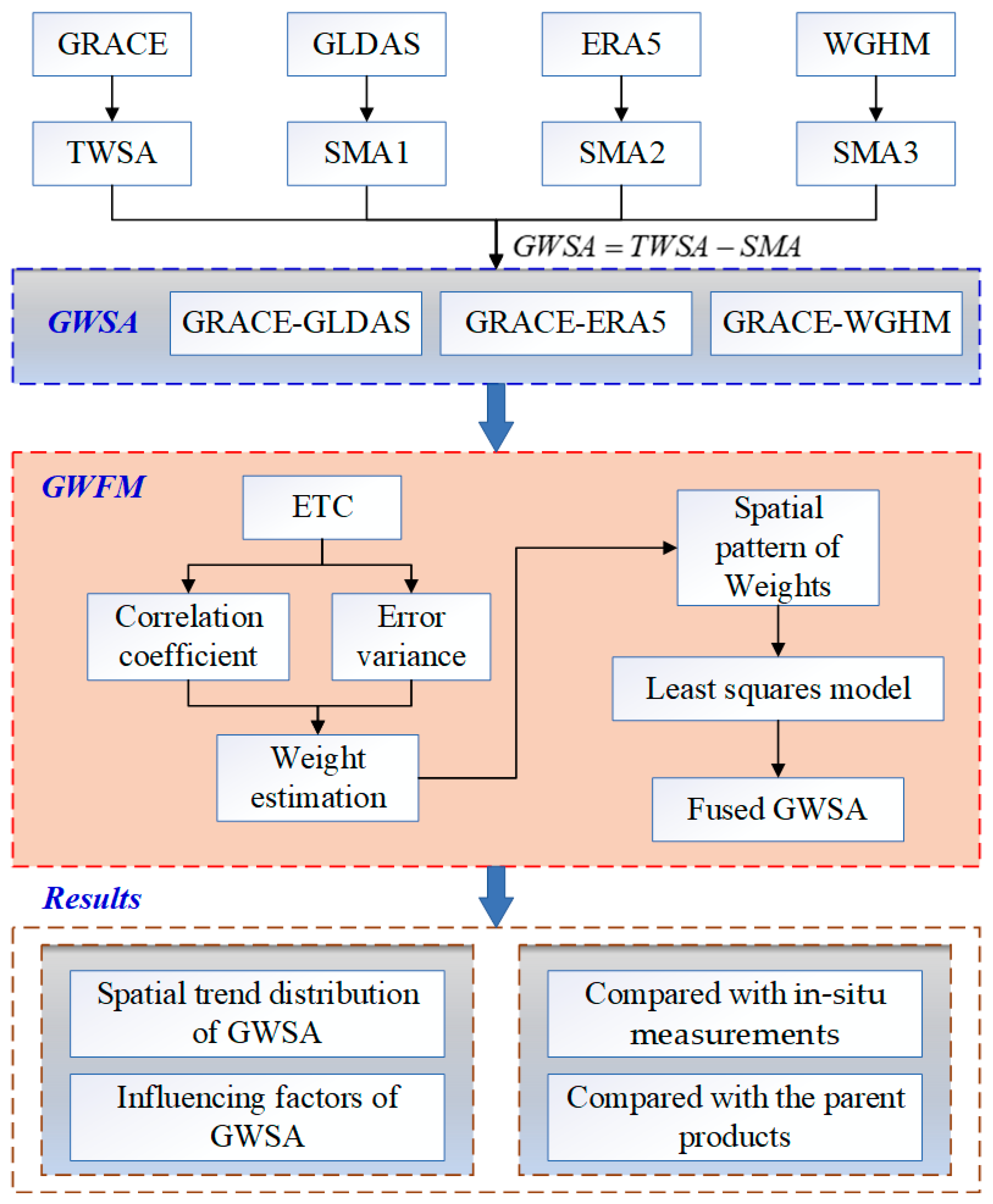
2.3.1. Construction of GWFM

Hydrological simulation typically needs to be calibrated by the “true” value of the target variable. However, it is difficult to obtain measured data in some areas because of the uneven distribution of monitoring points. ETC is a statistical method to estimate the correlation coefficient and the random-error variance of three independent datasets. The prerequisites for the TC approach are: (i) linearity between the true hydrological signal and the observations, (ii) signal and error stationarity, (iii) independency between the errors and the hydrological signal (error orthogonality), and (iv) independency between the errors of each dataset (zero-error cross-correlation) [35]. This study uses the error variance and squared correlation coefficient calculated by the ETC method to develop the GWFM. The error model is given by [35,40]:
S i = α i + β i Θ + ε i
where S i   ( i = 1 , 2 , 3 ) represents GWSA based on GRACE and three hydrological models; Θ denotes the unknown true hydrological signal; S i represents collocated measurement systems linearly related to the true unknown value, Θ ; α i and β i represent the least-squares intercepts and slope, respectively; and ε i represents additive zero-mean random noise.
Covariance estimation is used to solve random-error variance in this study. The covariances between the different datasets are given by [35,40]:
cov ( S i , S j ) = E ( S i S j ) E ( S i ) E ( S j ) = β i β j σ Θ 2 + β i cov ( Θ , ε j ) + β j cov ( Θ , ε i ) + cov ( ε i , ε j )
According to these four prerequisites of the TC approach, cov ( ε i , ε j ) = 0   ( i j ) , cov ( ε i , Θ ) = 0 ; the equation reduces to [35,40]:
C i j = cov ( S i , S j ) = β i β j σ Θ 2   ( i j ) β i 2 σ Θ 2 + σ ε i 2   ( i = j )
where σ ε i 2 represents the variance of random-error variance, ε i ; β i 2 σ Θ 2 denotes the sensitivity of datasets, S i , to changes in true signal. In other words, the higher β i , the stronger the response of datasets, S i , to hydrological signal. The sensitivity of each dataset can be calculated by combining their covariances [35,40]:
β i 2 σ Θ 2 = C 12 C 13 C 23 C 21 C 23 C 13 C 31 C 32 C 12
The error variance can be obtained by subtracting the sensitivity β i 2 σ Θ 2 of each dataset from their total variance [35,40]:
σ ε i 2 = C 11 C 12 C 13 C 23 C 22 C 21 C 23 C 13 C 33 C 31 C 32 C 12
ρ i , Θ 2 = β i 2 σ Θ 2 β i 2 σ Θ 2 + σ ε i 2 = S N R i S N R i + 1
S N R i = var ( S i ) var ( ε i ) = β i 2 σ Θ 2 σ ε i 2
where ρ i , Θ 2 represents the squared correlation coefficient and S N R represents the un-biased signal-to-noise ratio.
In this study, the error variance and squared correlation coefficient calculated by the above method are used to develop the GWFM. The detailed formula is as follows:
W i =   ρ i , Θ 2 / σ ε i 2 i = 1 n ρ i , Θ 2 / σ ε i 2   ( ρ i , Θ 2 > 0 , σ ε i 2 > 0 ) 1 / 3 ( ρ i , Θ 2 < 0 , σ ε i 2 < 0 )
Y model = W 1 M 1 + W 2 M 2 + W 3 M 3
where M i   ( i = 1 , 2 , 3 ) denotes the time series of the same position for the three datasets and W i denotes the weight of the corresponding time series, M i .

2.3.2. Estimation of GWSA Based on GRACE

Generally, GWSA can be estimated by subtracting CWS, SWE, and SM simulated by hydrologic models from the GRACE-derived TWS anomalies [4]. The detailed formula is as follows:
G W S A = T W S A S M A S W E A C W S A
where S M A , S W E A , and C W S A represent the storage anomalies of SM, SWE and CWS, respectively, relative to a reference period (the reference period is 2004–2009). Previous studies indicated that SM and GWS are the primary contributors to TWS changes and that variations in snow and ice, biomass, and surface water are relatively minor [9,19,58,59]. In addition, the selected study area is located in the arid region of northwest China and is mainly covered by bare land and gobi. Therefore, S W E and C W S can be ignored in this study.

2.3.3. Multiple Linear Regression of Time Series

To analyze the seasonal and secular trend of GWSA, multiple linear regression is used to analyze the temporal variability of GWSA. The regression model is given by [60]:
Y ( t ) = β 1 + β 2 t + β 3 sin ( π t ) + β 4 cos ( π t ) + β 5 sin ( 2 π t ) + β 6 cos ( 2 π t ) + ε
where Y ( t ) denotes GWSA at time t; β 1 and β 2 denote the constant offset and secular trend, respectively; β 3 and β 4 represent the annual signal; β 5 and β 6 represent semi-annual signals; and ε represents the model error. Meanwhile, the annual and semi-annual amplitude are computed as [60]:
a n n u a l   a m p l i t u d e = β 3 2 + β 4 2
s e m i a n n u a l   a m p l i t u d e = β 5 2 + β 6 2

2.3.4. Estimation of the Contribution to GWS

GRACE can monitor the temporal and spatial changes of TWS, including human factors and climate factors. In order to evaluate the contribution of different factors to GWS, a method is used to evaluate the contribution of these two factors, which can be computed as follows [61]:
G W S C c = G W S C G R A C E G W S C H
G W S C = G W S A t G W S A t 1
η H = G W S C H G W S C H + G W S C C
η C = G W S C C G W S C H + G W S C C
where G W S C C represents climate-driven GWS changes; G W S C G R A C E represents the annual GWS changes estimated by GRACE data; and G W S C H denotes the part of GWS changes induced by human factors. η H and η C denote the contribution of human and climatic factors to GWS changes, respectively. If η is positive, it provides a positive impact on GWS; otherwise, the opposite is true.

2.3.5. Evaluation Index

In this study, the correlation coefficient (CC), the root mean squared error (RMSE), and the Nash-Sutcliffe efficiency coefficient (NSE) are utilized to test the performance of this result [61,62,63].
C C = cov ( X ( t ) , Y ( t ) ) var [ X ( t ) ] var ( Y ( t ) )
R M S E = 1 n i = 1 n ( X ( t ) Y ( t ) ) 2
N S E = 1 i = 1 n ( X ( t ) Y ( t ) ) 2 i = 1 n ( X ( t ) X m e a n ) 2
where n denotes the total number of observations; X ( t ) and Y ( t ) denote measurements and simulated values, respectively; and X m e a n represents the mean of measurements. Considering inconsistent scales between different results, in situ groundwater-level measurements and simulated results should be normalized to [−1, 1].

3. Results

3.1. Experimental Verifications of the GWFM

It is necessary to test the performance of the GWFM before it is applied to the study area and the SYRB is chosen as the study area. The GWSA results based on GRACE observations and three hydrological models (namely GLDAS, ERA5, and WGHM) are introduced as the input data of the GWFM, and GWFM-based results are verified against in situ groundwater-level measurements.
Figure 3 represents the time series of GWSA estimated from the GWFM and three GRACE-based GWSA (hereafter GRACE−GLDAS, GRACE−ERA5, and GRACE−WGHM). Moreover, in situ groundwater-level measurements are also shown, and the shaded areas represent the uncertainties of GWFM-based GWSA. From the long-term variation of GWSA point of view, GWFM-based GWSA agree well with that, based on GRACE in terms of periodicity and seasonality. Furthermore, it is obvious that the long-term trends of GRACE-based and GWFM-based GWSA and in situ groundwater-level measurements are generally similar, showing a decreasing trend. However, there is a clear difference in phase between them (Figure 3). In other words, there is a clear time lag between GRACE-based GWSA and in situ groundwater-level measurements. Many previous studies have reported the time lag; for example, Thomas et al. [64] indicated that when the lag time was two months, the correlation between GRACE-based GWSA and in situ groundwater-level measurements reached a maximum in the Central Valley of California. Abou et al. [65] reported that there was a clear time lag between in situ groundwater-level measurements and GWSA based on GRACE in the Bakhtegan catchment. In order to explore the best lag time, this study uses GRACE−GLDAS and in situ groundwater-level measurements (S1–S5) (Table 2). The result shows that the highest correlation (CC = 0.59–0.72) can be found when the lag time is 4–5 months.
In order to explore the reliability of the GWFM, the lag time is set to 4 months, and GRACE-based (GRACE−GLDAS, GRACE−ERA5, and GRACE−WGHM) and GWFM-based results are compared with in situ groundwater-level measurements (Figure 4). The comparison indicates that the seasonality of GRACE-based and GWFM-based GWSA is consistent with in situ groundwater-level measurements, and the annual amplitude of GRACE−ERA5 is greater than that of GRACE−GLDAS and GRACE−WGHM. Furthermore, the amplitudes of in situ groundwater-level measurements (S1–S5) also display larger differences. For example, S3 shows a small amplitude change after 2011; the amplitude of S1 varies from −3 m to 5 m, and the amplitude of S5 is between −8 m and 16 m from the perspective of the long-term average.
In order to quantify the agreement between GWFM-based GWSA and in situ groundwater-level measurements, three metrics (CC, RMSE, and NSE) are calculated over the SYRB, as shown in Figure 5. This result shows that the agreement between GWFM-based GWSA and in situ groundwater-level measurements is much better than that based on GRACE. Additionally, the GWFM effectively improves the CC and NSE and decreases the RMSE. Specifically, the CC between GWFM-based GWSA and in situ groundwater-level measurements, S1, increases from 0.54 to 0.74, and the RMSE decreases from 0.44 to 0.39, the NSE increases from 0.11 to 0.54 relative to the original results. Compared with the mean value of in situ groundwater-level measurements (expressed by S6), similar improvements can also be seen for CC (9–40%), NSE (23–657%), and RMSE (9–28%). The above verification results indicate that reasonable GWSA estimates can be obtained through the GWFM in the SYRB. Therefore, it can give us confidence in applying this developed method to the HC, so as to better understand the temporal and spatial characteristics.

3.2. Comparison of GWSA

Figure 6 shows the annual, monthly, and seasonal scales of GRACE-based and GWFM-based GWSA from January 2003 to December 2016. The long-term trend of GRACE-based and GWFM-based GWSA shows a reasonable agreement, and four results also have a similar annual cycle. For the intra-annual changes of GWSA, the GWSA time series have a reasonable agreement; the anomalies are positive from May to August (Figure 6c). However, the values are negative for other months, and the only exception is the GRACE−GLDAS, always remaining negative. The main reason is that the HC is dry and less rainy, and ~80% of rainfall occurs during the period from May to September [66], which effectively recharges the groundwater. The HC is a well-known irrigated agricultural area in northwest China, but surface-water resources are scarce, and irrigation water mainly comes from groundwater. Therefore, a large amount of groundwater is pumped in spring and summer due to irrigation needs, which leads to a decrease in groundwater storage.
From the perspective of the long-term trend, GWSA reveals a significant downward trend over the study period. Notably, 2011 is a turning point, and the downward trend before 2011 is significantly higher than the trend after 2011. In order to clarify the difference between the four results, multivariate statistical analysis is used for the GWSA time series in the two time periods of 2003–2010 and 2011–2016 in the HC. Table 3 summarizes the evaluation indexes for the GWSA time series, including the long-term trend and annual amplitude. From 2003 to 2010, four GWSA downtrends range from 1.08 (GRACE−ERA5) to 4.17 (GRACE−GLDAS) mm/yr, which clearly indicates groundwater depletion in the HC during the period from 2003 to 2011. From 2011 to 2016, the results also show a downward trend (except GRACE−WGHM), and decline rates range from 0.46 (GWFM) to 0.70 (GRACE−ERA5) mm/yr, while GRACE−WGHM increased at a rate of 0.07 mm/yr. The rate of decline from 2011 to 2016 is significantly slower than that from 2003 to 2010, while the annual amplitude, compared with the previous period, increases significantly. This result may be related to the water policy in the area, such as Gansu Province gradually implementing the most stringent water-resource management system and measures of “points to areas, Hexi first” in 2011 [67].
The annual and semi-annual changes of time series can be analyzed by phasor diagrams, which show their amplitude and phase based on a reference period (in this study, the reference period is 2004–2009). The length of each vector represents the magnitude of amplitude, while the vector direction represents a phase. The bigger the difference between two vector directions and length, the greater the phase and amplitude difference between two time series. In other words, the phase difference can affect the magnitude of the correlation, and a difference in amplitude can affect variance agreement. In the case of annual amplitude and phases, GRACE−ERA5 has a higher annual amplitude than other results (shown in Figure 7a). Although the best amplitude agreement exists between GWFM-based result and GRACE−WGHM, the phase correspondence is poor, while GWFM-based GWSA agree well with GRACE−ERA5 at phase. In terms of semi-annual amplitude and phases (shown in Figure 7b), the phase and amplitude in GWSA from the GWFM show favorable agreement with GRACE−GLDAS, while the semi-annual phase and amplitude of GRACE−ERA5 are different from other results.

3.3. Spatial Pattern of Variation Trends in GWSA

Figure 8 shows the spatial distribution of GWSA based on GRACE and GWFM over the HC from 2003 to 2016. Among these results, GRACE−GLDAS shows that the area of GWS depletion has a higher downward trend and coverage, but the characteristics of spatial distribution in the Shule River Basin (SLRB) and the HRB are not distinct. GRACE−ERA5 shows obvious spatial-change characteristics, such as the D1 of the SLRB, the D2 of the HRB, and the D3 of the SYRB as the main GWS depleted areas (shown in Figure 8b). GRACE−WGHM shows a downward trend, high in the north and low in the south, but the overall spatial distribution shows no significant characteristic changes relative to other results. The GWFM highlights remarkable GWS depletion in the d1, d2, d3, and d4 (shown in Figure 8d), with the rates of about −4.22 mm/yr, −2.67 mm/yr, −3.77 mm/yr, and −5.06 mm/yr, respectively. It should be noted that, GRACE−ERA5 and the GWFM show opposite trends in the southeast of the SYRB, with the rates of 1.91 and −1.76 mm/yr, respectively.
The GWSA based on the GWFM is shown in Figure 9a, and the simple average result (average) of both GRACE-based GWSA is shown in Figure 9b. The main depletion areas of the two results are basically similar, but there is a large difference between the GWFM and average in the southeast of the SYRB (Df1 and df1), where the two trends are −1.76 mm/yr and 1.11 mm/yr, respectively. The government of Gansu Province announced Gulang County and Wuwei City as a GWS over-exploitation area, that is, the Df4 in Figure 9a, which is more consistent with the results of the GWFM. Therefore, the GWFM can effectively integrate the advantages of multiple models, retain the characteristics of specific regional changes, and provide a more accurate GWSA result relative to simple average results.

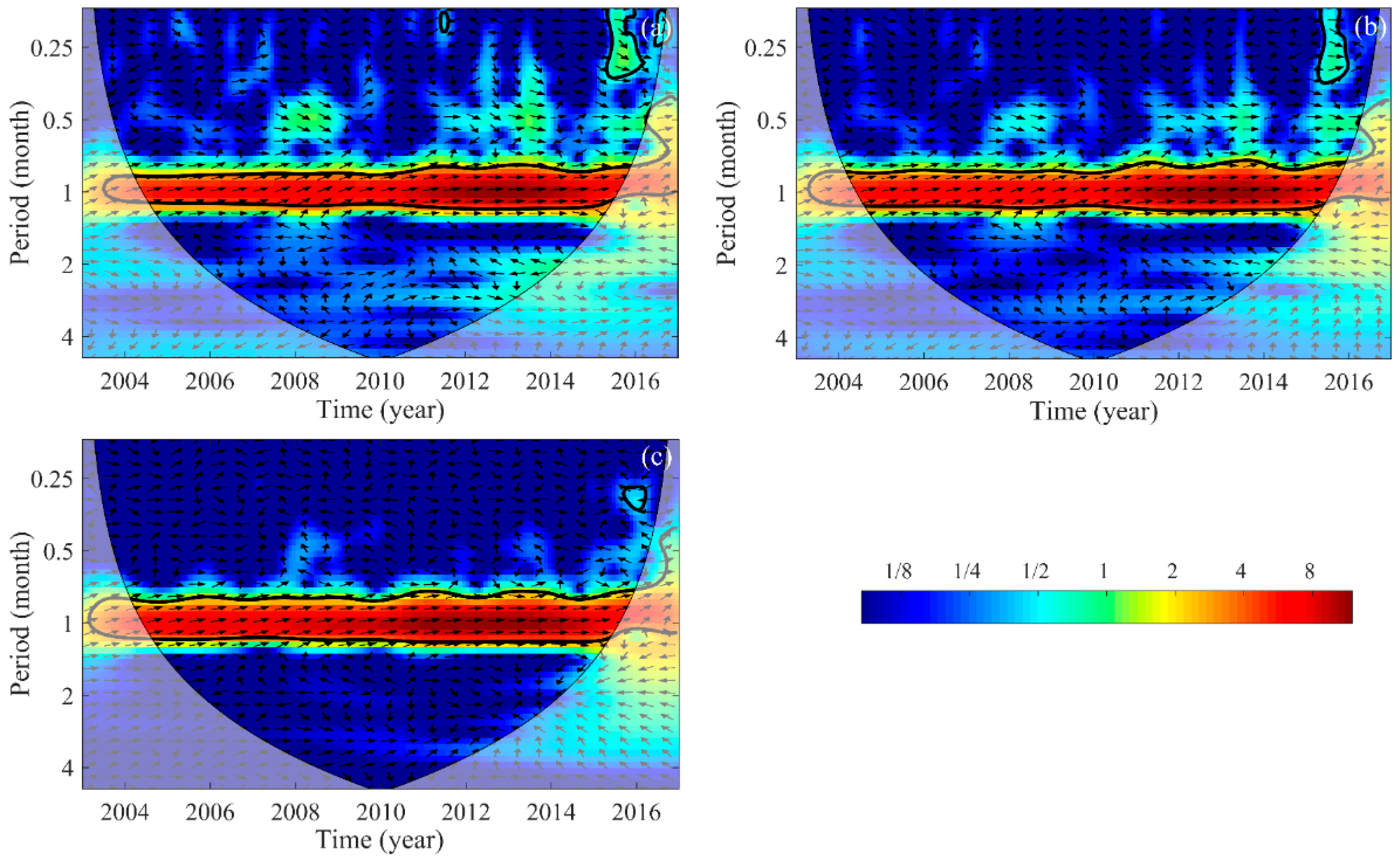
3.4. Response of GWSA to Climate Change

GWS changes are closely related to climate and human factors. Therefore, it is necessary to evaluate the relationship between GWFM-based GWSA and influencing factors in order to better understand the causes and development of groundwater depletion in the HC.
In the context of climate change, precipitation and evapotranspiration are the dominant factors that have the greatest impact on GWS [68]. Temperature changes lead to changes in evapotranspiration, which, in turn, lead to changes in GWS. The net recharge of groundwater is the difference between recharge and discharge [2]. Groundwater in the HC piedmont plain is mainly from the infiltration of surface runoff, which accounts for ~80% of total recharge [69], followed by precipitation and seepage of irrigation water. Groundwater discharge is mainly groundwater pumping and evapotranspiration of shallow groundwater [70].
To further analyze the detailed relationship between climatic factors and GWSA, cross-wavelet analysis is used in this study. Cross-wavelet transforms between GWSA and climatic factors in the HC are displayed in Figure 10. Figure 10a indicates that the correlations between precipitation and GWSA are strong in the HC during the period of 2003–2016, and it shows a statistically positive correlation between precipitation and GWSA at the 95% confidence level. Evapotranspiration and temperature also exhibit a strong positive correlation. In addition, GWSA and climatic factors all have a main resonance period of about 1 month.
Under the background of climate change, precipitation is the input of water, and evapotranspiration is the output of water in a region. Therefore, precipitation minus evapotranspiration (P−ET) can represent the net recharge of surface water and groundwater [71]. During 2003–2016, the maximum P−ET occurred in June-September, and the minimum in January-April and October-December (shown in Figure 11). P−ET shows a significant downward trend relative to other time periods during 2007–2016, resulting in a significant decrease in net recharge. Such shortage of precipitation will directly hinder the growth of vegetation and human production, and excessive evapotranspiration will further accelerate the loss of available water resources and disrupt the balance of the water cycle [72]. Although the net recharge in summer is positive during this period, groundwater is still in a state of declining, indicating that groundwater is not effectively recharged.
In addition, snowmelt is also an important factor in groundwater replenishment. In the context of climate change, snowmelt will increase. This impact means less snow accumulation in the winter and an earlier peak runoff in the spring [73]. Meanwhile, snowmelt is an important water source in Northwest China, which is of great significance to maintenance of ecological balance and sustainable development [74]. Li et al. [75] showed that from 1960 to 2010, the average annual runoff in the arid area of northwest China was increasing. Among them, the increased rate of runoff in the northern mountainous area of the Qilian Mountains was 1.48 × 10⁸ m3/10 a. Therefore, an increase in snowmelt will have a greater impact on runoff, which, in turn, affects recharge of groundwater.

3.5. Response of GWSA to Human Factors

In addition to climate factors, the impact of human factors on groundwater cannot be ignored. In the HC, water resources are scarce and unevenly distributed. During the crop-water demand season, a large amount of water resources is used for irrigation, when surface water for irrigation is limited, which will lead to a prominent contradiction between water supply and demand and inevitably lead to groundwater depletion. The HC has been undergoing tremendous changes over the past few decades. Niu et al. [76] showed that in the past 30 years, the increase in irrigation water consumption of farmland in the HRB had led to an average drop of about 1.86 m in groundwater. Zhou et al. [77] showed that as the area of farmland increased by 11.0%, the total irrigation water demand increased by 6.3% during the period from 2000 to 2010.
Figure 12 shows changes in groundwater withdrawal in the HC. During the entire survey period (2003–2016), the amount of groundwater withdrawal in the HRB is on a continuous upward trend, while other regions show a trend of a first decline and then an increase, reaching the lowest in 2009–2011, which is consistent with the change in precipitation. It is worth noting that even in the rainy season, GWS is in a state of decline. However, even in drier years, the amount of groundwater withdrawal is lower than in previous years, and the rate of decline in GWSA is higher than in the rainy season. This means that even when the amount of groundwater withdrawn is lower than in previous years, the amount of groundwater withdrawn is much higher than the amount of groundwater replenishment. If the use of water resources cannot be well improved, the area will continuously face the problem of groundwater depletion in the future.

4. Discussion

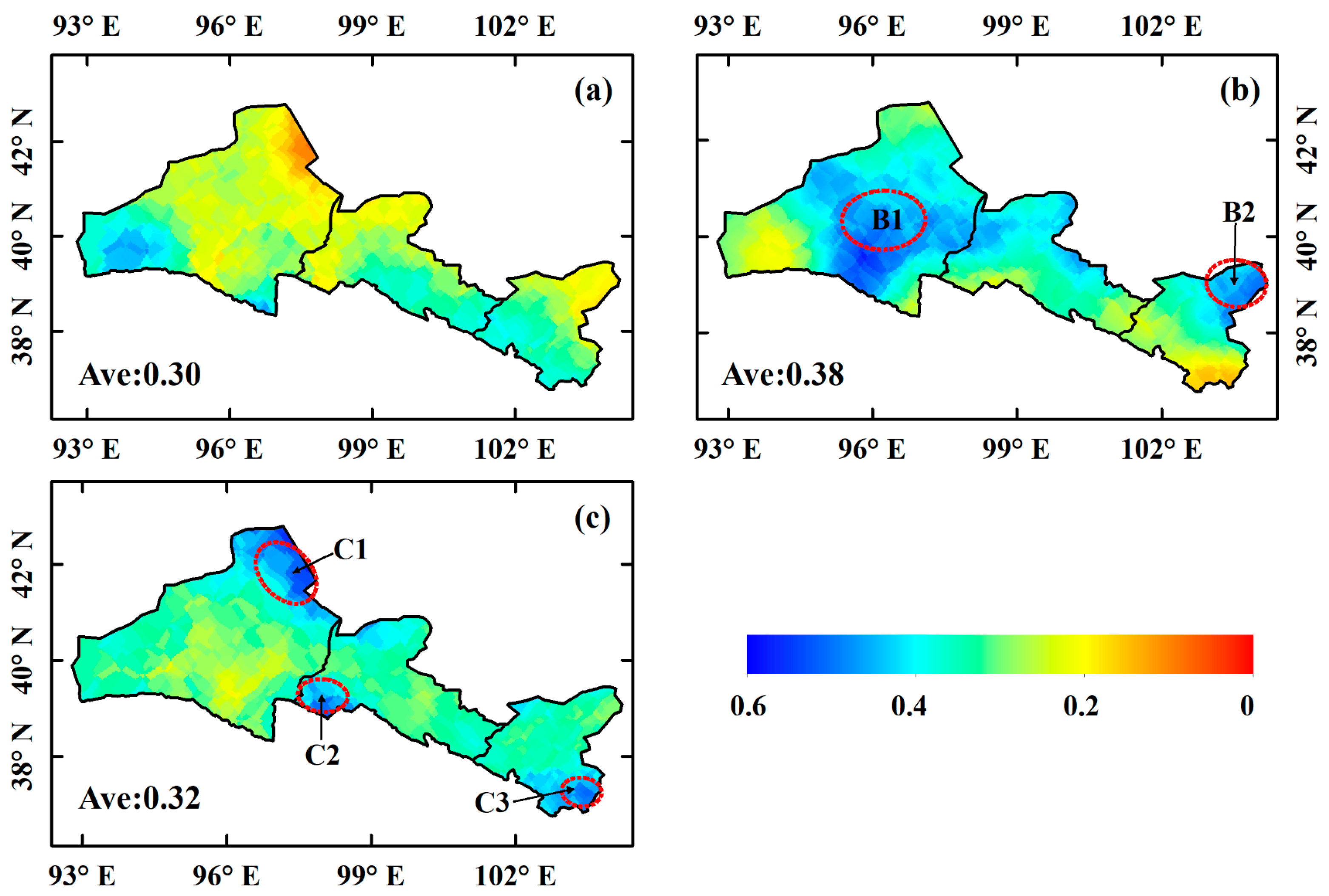
4.1. Spatial Distribution of Weight Index

The weighted fusion model is presented in this study, which can merge three GRACE-based GWSA. Specifically, the error variance and correlation coefficient of three GWSA derived by ETC are used for weight estimation. Then, three GWSA from different sources are merged by the least-squares framework. Therefore, it is necessary to discuss the weight of different original results.
Figure 13 shows the spatial distribution of the weights. This weight represents the relative contribution to the merged result. Among the three GRACE-based GWSA (including GRACE−GLDAS, GRACE−ERA5, and GRACE−WGHM), the largest average weight can be obtained by GRACE−ERA5 (0.38), followed by GRACE−WGHM (0.32) and GRACE−GLDAS (0.30). It is worth noting that there are apparent differences in spatial distribution, although the average weights of GRACE−GLDAS and GRACE−WGHM are relatively close. For example, GRACE−WGHM has larger weights than GRACE−GLDAS in C1, C2, and C3, accounting for about 0.50, 0.45, and 0.49, respectively. GRACE−GLDAS matches well with GRACE−WGHM in other regions. GRACE−ERA5 has higher weights relative to other results in B1 and B2. Furthermore, GRACE−ERA5 has a relatively high relative contribution to the merger result in most regions. These differences may be caused by different forced data and the parameters of the hydrological model [7,78]. In general, GRACE−ERA5 can accurately describe GWS changes in most areas of the HC from the perspective of single-model results.

4.2. Contributions of Different Factors to GWS

The contribution of climate factors and human factors to GWS has been evaluated using the method proposed in Section 2.3.4. Generally, the larger the value of η, the greater contribution it makes to GWS changes. The respective contributions are shown in Table 4.
As shown in Table 4, human factors are an important factor affecting GWS among climate and human factors in the HC and its subregions. For example, the impact of human activities shows a downward trend before 2010 and then begin to rise in the SYRB, which matches well with the change in trend of groundwater withdrawal in Figure 12. This is consistent with the conclusion drawn from other research conducted in this region, e.g., Liu et al. [44]. As for HRB, GWS changes affected by human factors show an upward trend with the increase in groundwater withdrawal. In the HC, the effects of climate change on GWS changes account for ~48%, while those of human activities contributed ~52%. This indicates that human activity has been the dominant factor driving the continuous reduction in groundwater. Wang et al. [5] reported that irrigation was continuously increased during the period of 2000–2016 in the HC. Moreover, Niu et al. [76] and Zhou et al. [77] also reported a similar situation in the subregions of the HC. This is consistent with our conclusion that human factors have become the dominant factor affecting GWS in the HC.

4.3. Limitation and Furture Work

In this study, there are some limitations, although reasonable results have been achieved. First, the GWFM proposed in this study is based on the same assumptions as the ETC method, such as error orthogonality and zero-error cross-correlation. Second, this study only uses GLDAS, ERA5, and WGHM, without considering other data sources. Third, there is only an eight-year overlap period with the GRACE data due to the short and discontinuous in situ groundwater-level measurement data. It is impossible to test the performance of the GWFM over a longer time frame.
In follow-up work, more data will be introduced to develop the model to compare and analyze GWSA in arid regions where in situ groundwater-level measurements are scarce. Furthermore, we will conduct a comparative analysis with the existing multi-model combination of technology to further improve the GWFM.

5. Conclusions

This study estimates GWSA by combining GRACE data with hydrological models. These data have their own unique characteristics and are developed for a global scale. Therefore, estimation of regional water-storage state generated by a single model may have greater uncertainty. In response to this problem, a GWFM is presented that can merge multi-source GWSA. The useful conclusions are as follows:
(1)
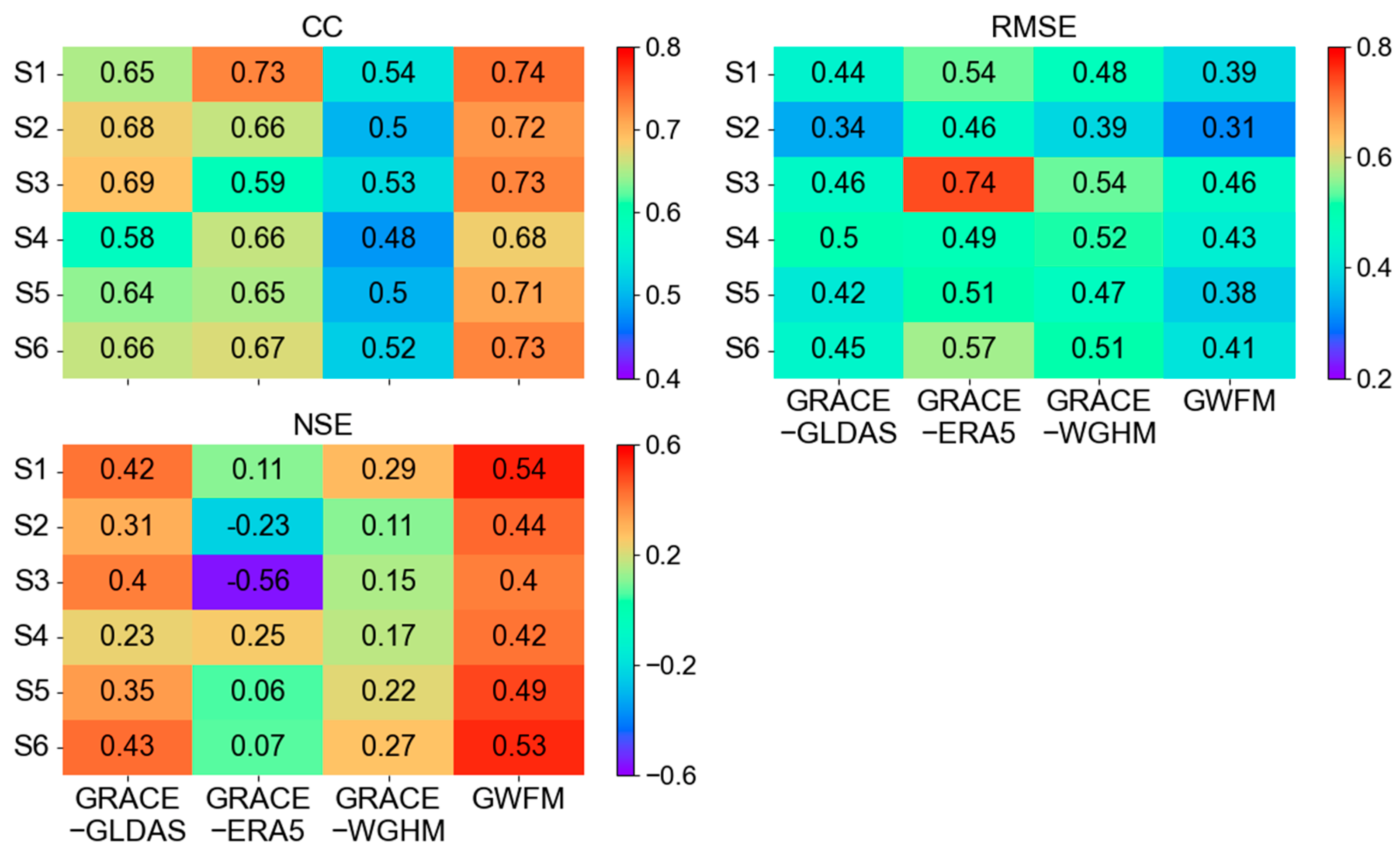
To obtain an accurate estimation of GWSA, this paper proposes a groundwater weighted fusion model. A comprehensive example is defined to verify the performance of the GWFM, and the superiority of the GWFM is verified by in situ groundwater-level measurements. The results show that the GWFM can effectively integrate the advantages of each data set sand produce a more reliable GWSA than the original results. Compared with GRACE-based GWSA, GWFM-based GWSA can obtain higher CC and NSE, CC increases by 9–40%, NSE increases by 23–657%, while RMSE decreases by 9–28%.
(2)
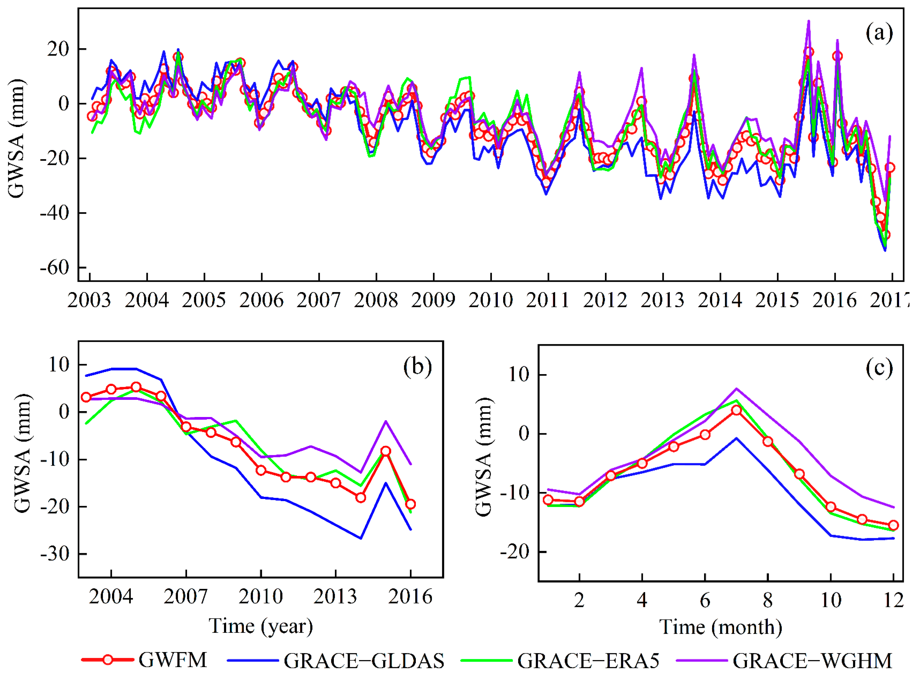
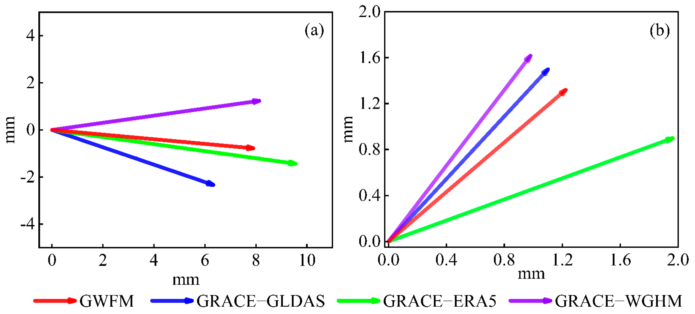
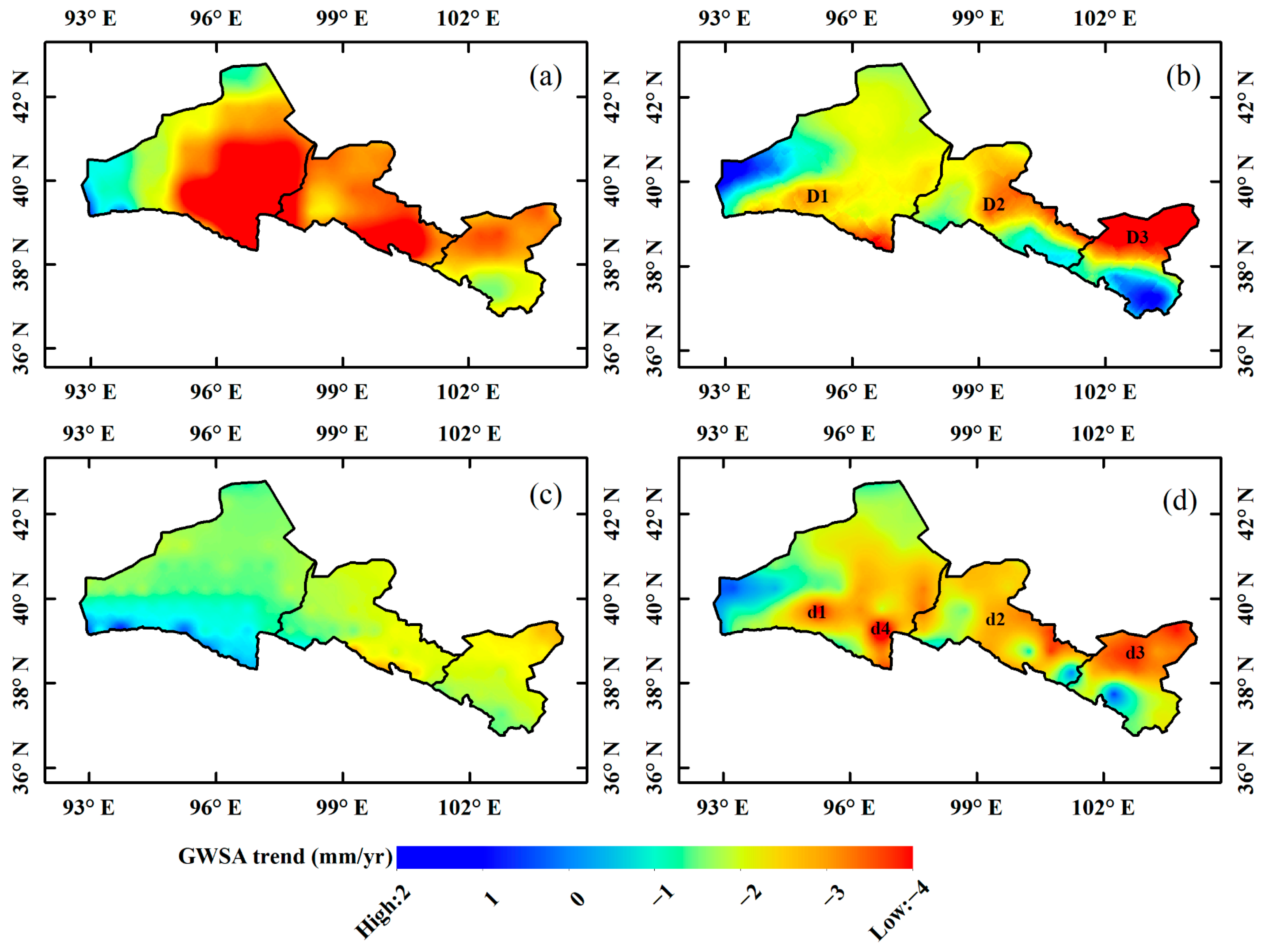
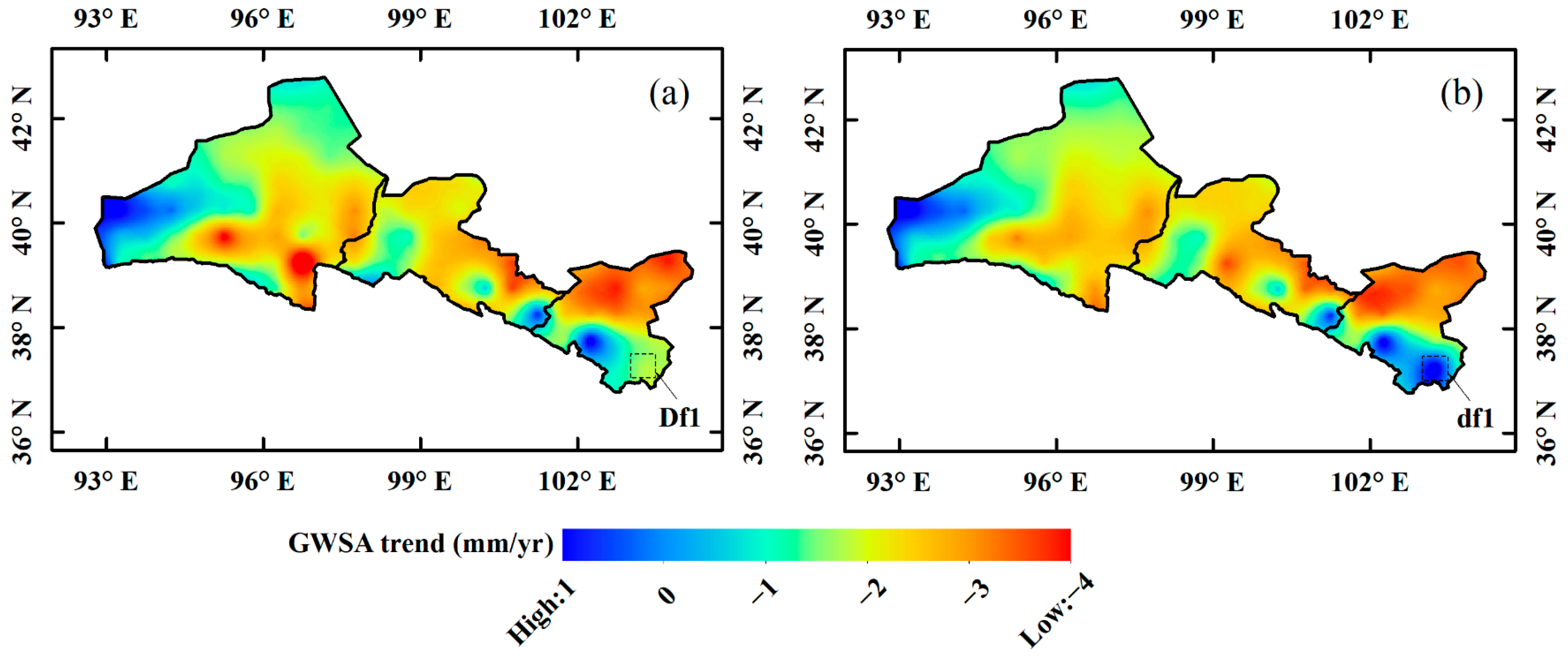
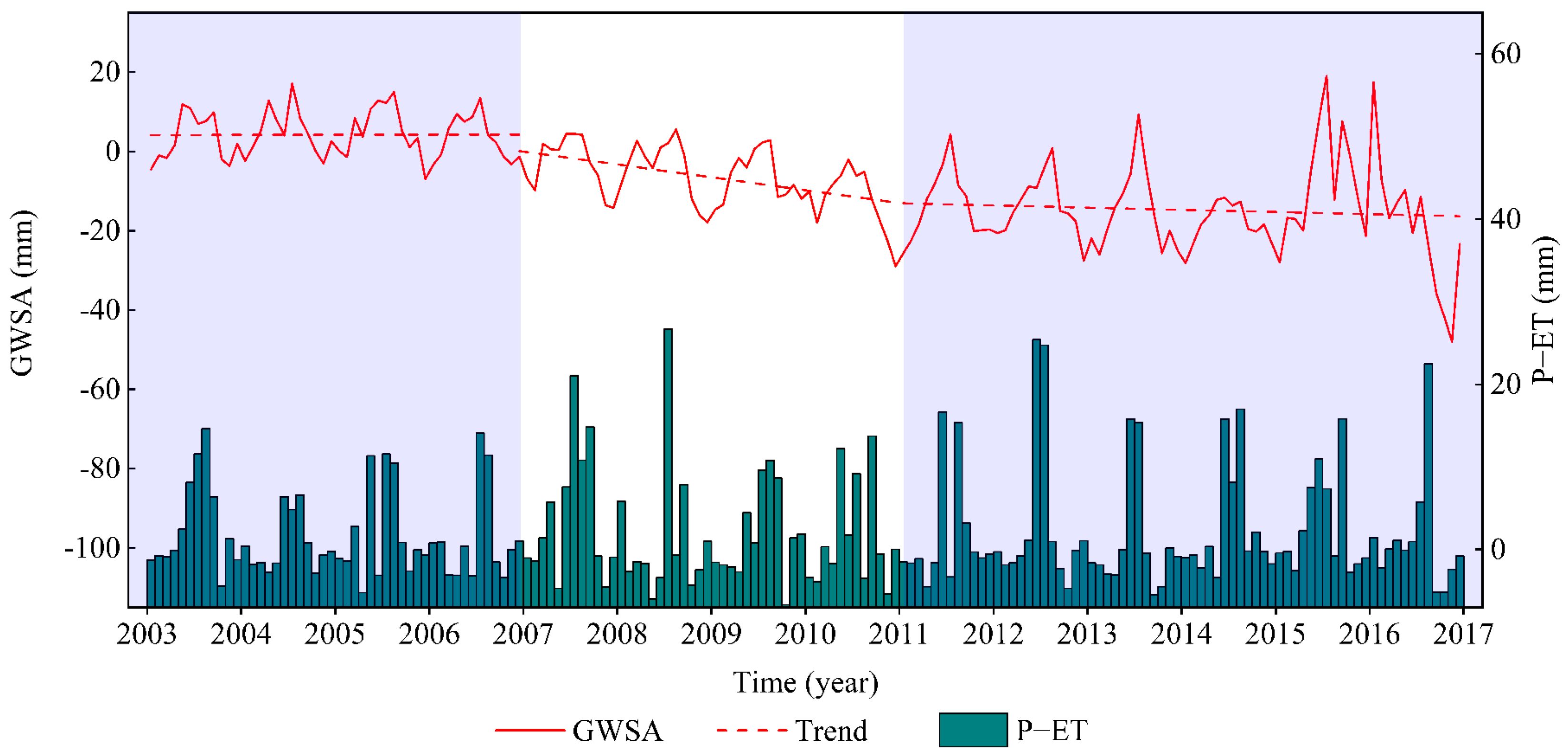
The GWSA result of the HC from 2003 to 2016 is calculated based on the GWFM. GWFM-based GWSA show an overall downward trend from 2003 to 2016, but 2011 is a turning point. From 2003 to 2010, there is a rapid downward trend, which is −2.37 ± 0.38 mm/yr, while the downward trend from 2011 to 2016 is significantly slowed, at −0.46 ± 1.35 mm/yr. This may be related to the local implementation of corresponding water-saving policies. In terms of spatial changes, in the central and southern part of the SLRB, the central part of the HRB and the northern part of the SYRB, which are the main GWS depleted areas, have a large downward trend. Furthermore, GWFM-based GWSA can better retain the characteristics of regional GWSA relative to the arithmetic average result, especially in the southeast of the SYRB.
(3)
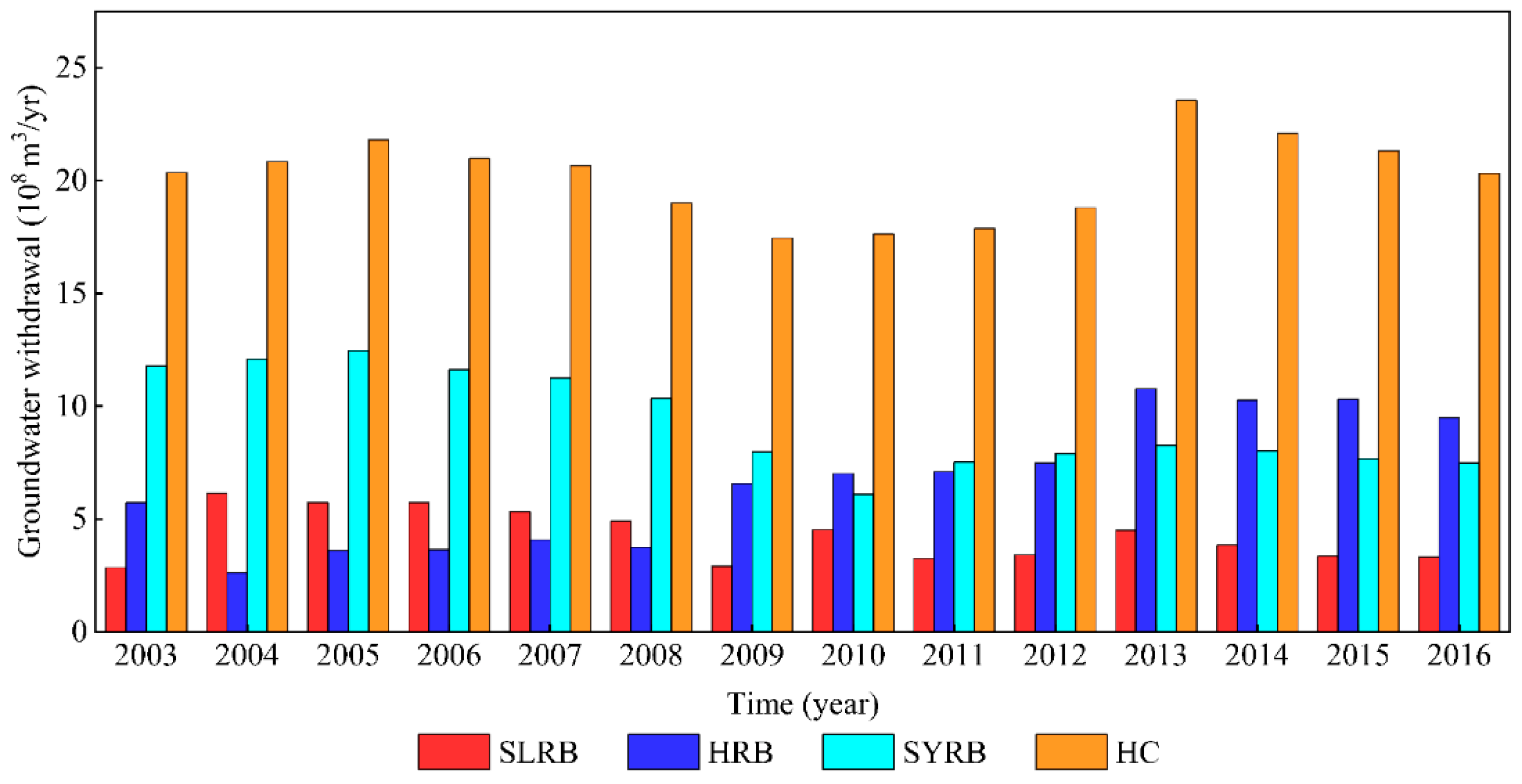
A simple and effective method is used to evaluate the contribution of climate factors and human factors to GWS. The results show that the amount of groundwater withdrawal has a significant impact on GWS, especially in the HRB, where the amount of groundwater withdrawal is increasing every year. As for the HC, the effects of climate change on GWS changes account for ~48%, while those of human activities contributed ~52%. In general, human activities, especially agricultural irrigation, have become the main reason for GWS decline in the HC.

Author Contributions

All authors collaborated to conduct this study. K.S., formal analysis, manuscript writing, and editing; W.Z. and W.Y.: supervision, project management, and editing; L.H. and Y.S., review and editing. All authors have read and agreed to the published version of the manuscript.

Funding

This work was supported by the National Natural Science Foundation of China under Grant (41774014, 41574014), the Liaoning Revitalization Talents Program under Grant (XLYC2002082), the Frontier Science and Technology Innovation Project and the Innovation Workstation Project of Science and Technology Commission of the Central Military Commission under Grant (085015), and the Outstanding Youth Fund of China Academy of Space Technology.

Institutional Review Board Statement

Not applicable.

Informed Consent Statement

Not applicable.

Data Availability Statement

No new data were created or analyzed in this study. Data sharing is not applicable to this article.

Acknowledgments

The authors greatly appreciate the institutions of CSR (http://www.csr.utexas.edu/grace/ (accessed on 1 July 2021)), which provided the GRACE mascon data. The authors would like to thank NASA for providing the dataset of GLDAS (https://disc.gsfc.nasa.gov/ (accessed on 1 July 2021)). The authors thank ECMWF (https://www.ecmwf.int/ (accessed on 1 July 2021) for the re-analysis data of the atmospheric pressure. The authors thank Hannes Muller Schmied for providing the hydrological outputs from the WGHM model. Finally, the authors also thank China Meteorological Administration (http://data.cma.cn/ (accessed on 10 August 2021)) for providing precipitation dataset. Kai Su, Wei Zheng, and Wenjie Yin contributed equally to this paper.

Conflicts of Interest

The authors declare no conflict of interest.

Abbreviations

AcronymFull Name
GRACEGravity Recovery and Climate Experiment
TWSterrestrial water storage
GWSgroundwater storage
GWSAgroundwater storage anomalies
GWFMgroundwater weighted fusion model
ETCextended triple collocation
HCHexi Corridor
SYRBShiyang River Basin
HRBHei River Basin
SLRBShule River Basin
SMsoil moisture
SWEsnow water equivalent
CWScanopy water storage
GLDASGlobal Land Data Assimilation System
WGHMWaterGAP Global Hydrology model
CIGEMChina Institute of Geological Environment Monitoring
CCcorrelation coefficient
RMSEroot mean squared error
NSENash-Sutcliffe efficiency coefficient

References

  1. Feng, W.; Zhong, M.; Lemoine, J.M.; Biancale, R.; Hsu, H.T.; Xia, J. Evaluation of groundwater depletion in North China using the Gravity Recovery and Climate Experiment (GRACE) data and ground-based measurements. Water Resour. Res. 2013, 49, 2110–2118. [Google Scholar] [CrossRef]
  2. Zhong, Y.; Zhong, M.; Mao, Y.; Ji, B. Evaluation of Evapotranspiration for Exorheic Catchments of China during the GRACE Era: From a Water Balance Perspective. Remote Sens. 2020, 12, 511. [Google Scholar] [CrossRef] [Green Version]
  3. Eamus, D.; Zolfaghar, S.; Villalobos Vega, R.; Cleverly, J.; Huete, A. Groundwater-dependent ecosystems: Recent insights from satellite and field-based studies. Hydrol. Earth Syst. Sci. 2015, 19, 4229–4256. [Google Scholar] [CrossRef] [Green Version]
  4. Frappart, F.; Ramillien, G. Monitoring groundwater storage changes using the Gravity Recovery and Climate Experiment (GRACE) Satellite Mission: A Review. Remote Sens. 2018, 10, 829. [Google Scholar] [CrossRef] [Green Version]
  5. Wang, S.; Liu, H.; Yu, Y.; Zhao, W.; Yang, Q.; Liu, J. Evaluation of groundwater sustainability in the arid Hexi Corridor of Northwestern China, using GRACE, GLDAS and measured groundwater data products. Sci. Total Environ. 2020, 705, 135829. [Google Scholar] [CrossRef]
  6. Chen, J.; Famigliett, J.S.; Scanlon, B.R.; Rodell, M. Groundwater Storage Changes: Present Status from GRACE Observations. Surv. Geophys. 2016, 37, 397–417. [Google Scholar] [CrossRef]
  7. Yin, W.; Li, T.; Zheng, W.; Hu, L.; Han, S.C.; Tangdamrongsub, N.; Šprlák, M.; Huang, Z. Improving regional groundwater storage estimates from GRACE and global hydrological models over Tasmania, Australia. Hydrogeol. J. 2020, 28, 1809–1825. [Google Scholar] [CrossRef]
  8. Tapley, B.D.; Bettadpur, S.; Ries, J.C.; Thompson, P.F.; Watkins, M.M. GRACE measurements of mass variability in the earth system. Science 2004, 305, 503–505. [Google Scholar] [CrossRef] [Green Version]
  9. Rodell, M.; Velicogna, I.; Famiglietti, J.S. Satellite-based estimates of groundwater depletion in India. Nature 2009, 460, 999–1002. [Google Scholar] [CrossRef] [Green Version]
  10. Rodell, M.; Famiglietti, J.S. An analysis of terrestrial water storage variations in Illinois with implications for the Gravity Recovery and Climate Experiment (GRACE). Water Resour. Res. 2001, 37, 1327–1339. [Google Scholar] [CrossRef] [Green Version]
  11. Chen, H.; Zhang, W.; Nie, N.; Guo, Y. Long-term groundwater storage variations estimated in the Songhua River Basin by using GRACE products, land surface models, and in-situ observations. Sci. Total Environ. 2019, 649, 372–387. [Google Scholar] [CrossRef]
  12. Tangdamrongsub, N.; Han, S.C.; Decker, M.; Yeo, I.Y.; Kim, H. On the use of the GRACE normal equation of inter-satellite tracking data for estimation of soil moisture and groundwater in Australia. Hydrol. Earth Syst. Sci. 2018, 22, 1811–1829. [Google Scholar] [CrossRef] [Green Version]
  13. Rodell, M.; Houser, P.R.; Jambor, U.; Gottschalck, J.; Mitchell, K.; Meng, C.J.; Arsenault, K.; Cosgrove, B.; Radakovich, J.; Bosilovich, M.; et al. The global land data assimilation system. Bull. Am. Meteorol. Soc. 2004, 85, 381–394. [Google Scholar] [CrossRef] [Green Version]
  14. Döll, P.; Kaspar, F.; Lehner, B. A global hydrological model for deriving water availability indicators: Model tuning and validation. J. Hydrol. 2003, 270, 105–134. [Google Scholar] [CrossRef]
  15. Xu, L.; Chen, N.; Zhang, X.; Moradkhani, H.; Zhang, C.; Hu, C. In-situ and triple-collocation based evaluations of eight global root zone soil moisture products. Remote Sens. Environ. 2021, 254, 112248. [Google Scholar] [CrossRef]
  16. Hersbach, H.; Bell, B.; Berrisford, P.; Hirahara, S.; Horányi, A.; Muñoz-Sabater, J.; Nicolas, J.; Peubey, C.; Radu, R.; Schepers, D.; et al. The ERA5 global reanalysis. Q. J. R. Meteorol. Soc. 2020, 146, 1999–2049. [Google Scholar] [CrossRef]
  17. Scanlon, B.R.; Longuevergne, L.; Long, D. Ground referencing GRACE satellite estimates of groundwater storage changes in the California Central Valley, USA. Water Resour. Res. 2012, 48, 4520. [Google Scholar] [CrossRef] [Green Version]
  18. Famiglietti, J.; Lo, M.; Ho, S.; Bethune, J.; Anderson, K.; Syed, T.; Swenson, S.; De Linage, C.; Rodell, M. Satellites Measure Recent Rates of Groundwater Depletion in California’s Central Valley. Geophys. Res. Lett. 2011, 38. [Google Scholar] [CrossRef] [Green Version]
  19. Long, D.; Chen, X.; Scanlon, B.R.; Wada, Y.; Hong, Y.; Singh, V.P.; Chen, Y.; Wang, C.; Han, Z.; Yang, W. Have GRACE satellites overestimated groundwater depletion in the Northwest India Aquifer? Sci. Rep. 2016, 6, 24398. [Google Scholar] [CrossRef]
  20. Bhanja, S.N.; Mukherjee, A.; Saha, D.; Velicogna, I.; Famiglietti, J.S. Validation of GRACE based groundwater storage anomaly using in-situ groundwater level measurements in India. J. Hydrol. 2016, 543, 729–738. [Google Scholar] [CrossRef]
  21. Huang, Z.; Pan, Y.; Gong, H.; Yeh, P.J.F.; Li, X.; Zhou, D.; Zhao, W. Subregional-scale groundwater depletion detected by GRACE for both shallow and deep aquifers in North China Plain. Geophys. Res. Lett. 2015, 42, 1791–1799. [Google Scholar] [CrossRef]
  22. Moiwo, J.P.; Tao, F.; Lu, W. Analysis of satellite-based and in situ hydro-climatic data depicts water storage depletion in North China Region. Hydrol. Process. 2013, 27, 1011–1020. [Google Scholar] [CrossRef]
  23. Agutu, N.O.; Awange, J.L.; Ndehedehe, C.; Kirimi, F.; Kuhn, M. GRACE-derived groundwater changes over Greater Horn of Africa: Temporal variability and the potential for irrigated agriculture. Sci. Total Environ. 2019, 693, 133467. [Google Scholar] [CrossRef]
  24. Hu, Z.; Zhou, Q.; Chen, X.; Chen, D.; Li, J.; Guo, M.; Yin, G.; Duan, Z. Groundwater Depletion Estimated from GRACE: A Challenge of Sustainable Development in an Arid Region of Central Asia. Remote Sens. 2019, 11, 1908. [Google Scholar] [CrossRef] [Green Version]
  25. Xiao, R.; He, X.; Zhang, Y.; Ferreira, V.G.; Chang, L. Monitoring Groundwater Variations from Satellite Gravimetry and Hydrological Models: A Comparison with in-situ Measurements in the Mid-Atlantic Region of the United States. Remote Sens. 2015, 7, 686–703. [Google Scholar] [CrossRef] [Green Version]
  26. Duan, Q.; Ajami, N.K.; Gao, X.; Sorooshian, S. Multi-model ensemble hydrologic prediction using Bayesian model averaging. Adv. Water Resour. 2007, 30, 1371–1386. [Google Scholar] [CrossRef] [Green Version]
  27. Mehrnegar, N.; Jones, O.; Singer, M.B.; Schumacher, M.; Bates, P.; Forootan, E. Comparing global hydrological models and combining them with GRACE by dynamic model data averaging (DMDA). Adv. Water Resour. 2020, 138, 103528. [Google Scholar] [CrossRef]
  28. van Dijk, A.; Renzullo, L.; Wada, Y.; Tregoning, P. A global water cycle reanalysis (2003–2012) merging satellite gravimetry and altimetry observations with a hydrological multi-model ensemble. Hydrol. Earth Syst. Sci. 2014, 18, 2955–2973. [Google Scholar] [CrossRef] [Green Version]
  29. Soltani, S.S.; Ataie-Ashtiani, B.; Simmons, C.T. Review of assimilating GRACE terrestrial water storage data into hydrological models: Advances, challenges and opportunities. Earth-Sci. Rev. 2021, 213, 103487. [Google Scholar] [CrossRef]
  30. Dumedah, G.; Walker, J.P. Assessment of land surface model uncertainty: A crucial step towards the identification of model weaknesses. J. Hydrol. 2014, 519, 1474–1484. [Google Scholar] [CrossRef]
  31. Tangdamrongsub, N.; Han, S.-C.; Yeo, I.-Y.; Dong, J.; Steele-Dunne, S.C.; Willgoose, G.; Walker, J.P. Multivariate data assimilation of GRACE, SMOS, SMAP measurements for improved regional soil moisture and groundwater storage estimates. Adv. Water Resour. 2020, 135, 103477. [Google Scholar] [CrossRef]
  32. Shamseldin, A.Y.; O’Connor, K.M.; Liang, G.C. Methods for combining the outputs of different rainfall–runoff models. J. Hydrol. 1997, 197, 203–229. [Google Scholar] [CrossRef]
  33. Long, D.; Pan, Y.; Zhou, J.; Chen, Y.; Hou, X.; Hong, Y.; Scanlon, B.R.; Longuevergne, L. Global analysis of spatiotemporal variability in merged total water storage changes using multiple GRACE products and global hydrological models. Remote Sens. Environ. 2017, 192, 198–216. [Google Scholar] [CrossRef]
  34. Shamseldin, A.Y.; O’Connor, K.M. A real-time combination method for the outputs of different rainfall-runoff models. Hydrol. Sci. J. 1999, 44, 895–912. [Google Scholar] [CrossRef]
  35. Gruber, A.; Su, C.H.; Zwieback, S.; Crow, W.; Dorigo, W.; Wagner, W. Recent advances in (soil moisture) triple collocation analysis. Int. J. Appl. Earth Obs. Geoinf. 2016, 45, 200–211. [Google Scholar] [CrossRef]
  36. Rusli, S.R.; Weerts, A.H.; Taufiq, A.; Bense, V.F. Estimating water balance components and their uncertainty bounds in highly groundwater-dependent and data-scarce area: An example for the Upper Citarum basin. J. Hydrol. Reg. Stud. 2021, 37, 100911. [Google Scholar] [CrossRef]
  37. Khaki, M.; Awange, J.; Forootan, E.; Kuhn, M. Understanding the association between climate variability and the Nile’s water level fluctuations and water storage changes during 1992–2016. Sci. Total Environ. 2018, 645, 1509–1521. [Google Scholar] [CrossRef] [Green Version]
  38. Nigatu, Z.M.; Fan, D.; You, W. GRACE products and land surface models for estimating the changes in key water storage components in the Nile River Basin. Adv. Space Res. 2021, 67, 1896–1913. [Google Scholar] [CrossRef]
  39. Yin, G.; Park, J. The use of triple collocation approach to merge satellite- and model-based terrestrial water storage for flood potential analysis. J. Hydrol. 2021, 127197. [Google Scholar] [CrossRef]
  40. McColl, K.A.; Vogelzang, J.; Konings, A.G.; Entekhabi, D.; Piles, M.; Stoffelen, A. Extended triple collocation: Estimating errors and correlation coefficients with respect to an unknown target. Geophys. Res. Lett. 2014, 41, 6229–6236. [Google Scholar] [CrossRef] [Green Version]
  41. Li, X.; Tong, L.; Niu, J.; Kang, S.; Du, T.; Li, S.; Ding, R. Spatio-temporal distribution of irrigation water productivity and its driving factors for cereal crops in Hexi Corridor, Northwest China. Agric. Water Manag. 2017, 179, 55–63. [Google Scholar] [CrossRef]
  42. Wang, L.; Dong, Y.; Xu, Z. A synthesis of hydrochemistry with an integrated conceptual model for groundwater in the Hexi Corridor, northwestern China. J. Asian Earth Sci. 2017, 146, 20–29. [Google Scholar] [CrossRef]
  43. Chang, G.; Wang, L.; Meng, L.; Zhang, W. Farmers’ attitudes toward mandatory water-saving policies: A case study in two basins in northwest China. J. Environ. Manag. 2016, 181, 455–464. [Google Scholar] [CrossRef]
  44. Liu, X.; Hu, L.; Sun, K.; Yang, Z.; Sun, J.; Yin, W. Improved Understanding of Groundwater Storage Changes under the Influence of River Basin Governance in Northwestern China Using GRACE Data. Remote Sens. 2021, 13, 2672. [Google Scholar] [CrossRef]
  45. Hao, Y.; Xie, Y.; Ma, J.; Zhang, W. The critical role of local policy effects in arid watershed groundwater resources sustainability: A case study in the Minqin oasis, China. Sci. Total Environ. 2017, 601–602, 1084–1096. [Google Scholar] [CrossRef]
  46. Stoffelen, A. Toward the true near-surface wind speed: Error modeling and calibration using triple collocation. J. Geophys. Res. Ocean. 1998, 103, 7755–7766. [Google Scholar] [CrossRef]
  47. Guan, Q.; Yang, L.; Pan, N.; Lin, J.; Xu, C.; Wang, F.; Liu, Z. Greening and Browning of the Hexi Corridor in Northwest China: Spatial Patterns and Responses to Climatic Variability and Anthropogenic Drivers. Remote Sens. 2018, 10, 1270. [Google Scholar] [CrossRef] [Green Version]
  48. Fu, J.; Niu, J.; Kang, S.; Adeloye, A.J.; Du, T. Crop production in the Hexi Corridor challenged by future climate change. J. Hydrol. 2019, 579, 124197. [Google Scholar] [CrossRef]
  49. Bao, C.; Fang, C. Water resources constraint force on urbanization in water deficient regions: A case study of the Hexi Corridor, arid area of NW China. Ecol. Econ. 2007, 62, 508–517. [Google Scholar] [CrossRef]
  50. Ji, X.; Kang, E.; Chen, R.; Zhao, W.; Zhang, Z.; Jin, B. The impact of the development of water resources on environment in arid inland river basins of Hexi region, Northwestern China. Environ. Geol. 2006, 50, 793–801. [Google Scholar] [CrossRef]
  51. Yang, L.; Feng, Q.; Adamowski, J.F.; Deo, R.C.; Yin, Z.; Wen, X.; Tang, X.; Wu, M. Causality of climate, food production and conflict over the last two millennia in the Hexi Corridor, China. Sci. Total Environ. 2020, 713, 136587. [Google Scholar] [CrossRef]
  52. Save, H.; Bettadpur, S.; Tapley, B. High resolution CSR GRACE RL05 mascons. J. Geophys. Res. Solid Earth 2016, 121, 7547–7569. [Google Scholar] [CrossRef]
  53. Save, H.; Bettadpur, S.; Tapley, B. Reducing errors in the GRACE gravity solutions using regularization. J. Geod. 2012, 86, 695–711. [Google Scholar] [CrossRef]
  54. Scanlon, B.R.; Zhang, Z.; Save, H.; Wiese, D.N.; Landerer, F.W.; Long, D.; Longuevergne, L.; Chen, J. Global evaluation of new GRACE mascon products for hydrologic applications. Water Resour. Res. 2016, 52, 9412–9429. [Google Scholar] [CrossRef]
  55. Güntner, A.; Stuck, J.; Werth, S.; Doell, P.; Verzano, K.; Merz, B. A global analysis of temporal and spatial variations in continental water storage. Water Resour. Res. 2007, 43, 687–696. [Google Scholar] [CrossRef]
  56. Muñoz Sabater, J. ERA5-Land Monthly Averaged Data from 1981 to Present. Copernicus Climate Change Service (C3S) Climate Data Store (CDS). Available online: https://doi.org/10.24381/cds.68d2bb3 (accessed on 1 July 2021).
  57. Hutchinson, M.F. Interpolation of rainfall data with thin plate smoothing splines-Part I: Two dimensional smoothing of data with short range correlation. J. Geogr. Inf. Decis. Anal. 1998, 2, 139–151. [Google Scholar]
  58. Rodell, M.; Chao, B.F.; Au, A.Y.; Kimball, J.S.; McDonald, K.C. Global biomass variation and Its geodynamic effects: 1982–98. Earth Interact. 2005, 9, 1–19. [Google Scholar] [CrossRef] [Green Version]
  59. Strassberg, G.; Scanlon, B.R.; Chambers, D. Evaluation of groundwater storage monitoring with the GRACE satellite: Case study of the High Plains aquifer, central United States. Water Resour. Res. 2009, 45, W05410. [Google Scholar] [CrossRef] [Green Version]
  60. Yang, P.; Xia, J.; Zhan, C.; Qiao, Y.; Wang, Y. Monitoring the spatio-temporal changes of terrestrial water storage using GRACE data in the Tarim River basin between 2002 and 2015. Sci. Total Environ. 2017, 595, 218–228. [Google Scholar] [CrossRef]
  61. Xie, J.; Xu, Y.; Wang, Y.; Gu, H.; Wang, F.; Pan, S. Influences of climatic variability and human activities on terrestrial water storage variations across the Yellow River basin in the recent decade. J. Hydrol. 2019, 579, 124218. [Google Scholar] [CrossRef]
  62. Abhishek; Kinouchi, T. Synergetic application of GRACE gravity data, global hydrological model, and in-situ observations to quantify water storage dynamics over Peninsular India during 2002–2017. J. Hydrol. 2021, 596, 126069. [Google Scholar] [CrossRef]
  63. Moriasi, D.N.; Arnold, J.G.; Van Liew, M.W.; Bingner, R.L.; Harmel, R.D.; Veith, T.L. Model evaluation guidelines for systematic Quantification of Accuracy in watershed simulations. Trans. ASABE 2007, 50, 885–900. [Google Scholar] [CrossRef]
  64. Thomas, B.; Famiglietti, J.; Landerer, F.; Wiese, D.; Molotch, N.; Argus, D. GRACE groundwater drought index: Evaluation of California Central Valley groundwater drought. Remote Sens. Environ. 2017, 198, 384–392. [Google Scholar] [CrossRef]
  65. Abou Zaki, N.; Torabi Haghighi, A.; Rossi, P.; Tourian, M.; Klöve, B. Monitoring groundwater storage depletion using Gravity Recovery and Climate Experiment (GRACE) data in Bakhtegan Catchment, Iran. Water 2019, 11, 1456. [Google Scholar] [CrossRef] [Green Version]
  66. Yang, B.; Qin, C.; Bräuning, A.; Burchardt, I.; Liu, J. Rainfall history for the Hexi Corridor in the Arid Northwest China during the past 620 years derived from tree rings. Int. J. Climatol. 2011, 31, 1166–1176. [Google Scholar] [CrossRef]
  67. Zhang, S.; Zhang, Q.; Liu, Z.; Gao, Z.; Qi, D. Practice and exploration of implementing the strictest water resources management system in Gansu Province. China Water Conserv. 2011, 09, 35–37. (In Chinese) [Google Scholar]
  68. Su, Y.; Guo, B.; Zhou, Z.; Zhong, Y.; Min, L. Spatio-temporal variations in groundwater revealed by GRACE and Its driving factors in the Huang-Huai-Hai Plain, China. Sensors 2020, 20, 922. [Google Scholar] [CrossRef] [Green Version]
  69. Ding, H.; Zhang, J.; Lv, Z.; Yang, K.; Li, J.; Niu, X. Characteristics and Cycle Conversion of Water Resources in the Hexi Corridor. Arid Zone Res. 2006, 02, 241–248. (In Chinese) [Google Scholar]
  70. Liu, M.; Jiang, Y.; Xu, X.; Huang, Q.; Huo, Z.; Huang, G. Long-term groundwater dynamics affected by intense agricultural activities in oasis areas of arid inland river basins, Northwest China. Agric. Water Manag. 2018, 203, 37–52. [Google Scholar] [CrossRef]
  71. Byrne, M.P.; O’Gorman, P.A. The response of precipitation minus evapotranspiration to climate warming: Why the “Wet-Get-Wetter, Dry-Get-Drier” scaling does not hold over land. J. Clim. 2015, 28, 8078–8092. [Google Scholar] [CrossRef]
  72. Buma, W.; Lee, S.I. Multispectral image-based estimation of drought patterns and intensity around Lake Chad, Africa. Remote Sens. 2019, 11, 2534. [Google Scholar] [CrossRef] [Green Version]
  73. Barnett, T.P.; Adam, J.C.; Lettenmaier, D.P. Potential impacts of a warming climate on water availability in snow-dominated regions. Nature 2005, 438, 303–309. [Google Scholar] [CrossRef]
  74. Wang, Y.; Qin, D. Influence of climate change and human activity on water resources in arid region of Northwest China: An overview. Adv. Clim. Change Res. 2017, 8, 268–278. [Google Scholar] [CrossRef]
  75. Li, B.; Chen, Y.; Chen, Z.; Li, W. The effect of climate change during snowmelt period on streamflow in the mountainous areas of Northwest China. Acta Geogr. Sin. 2012, 67, 1461–1470. (In Chinese) [Google Scholar]
  76. Niu, J.; Zhu, X.G.; Parry, M.A.J.; Kang, S.; Du, T.; Tong, L.; Ding, R. Environmental burdens of groundwater extraction for irrigation over an inland river basin in Northwest China. J. Clean. Prod. 2019, 222, 182–192. [Google Scholar] [CrossRef] [Green Version]
  77. Zhou, D.; Wang, X.; Shi, M. Human driving forces of Oasis expansion in Northwestern China during the last decade—A case study of the Heihe River Basin. Land Degrad. Dev. 2017, 28, 412–420. [Google Scholar] [CrossRef]
  78. Long, D.; Scanlon, B.R.; Longuevergne, L.; Sun, A.Y.; Fernando, D.N.; Save, H. GRACE satellite monitoring of large depletion in water storage in response to the 2011 drought in Texas. Geophys. Res. Lett. 2013, 40, 3395–3401. [Google Scholar] [CrossRef] [Green Version]
Figure 1. Information summary of the Hexi corridor: (a) geographical location, (b) annual precipitation, (c) digital elevation and distribution of groundwater-level monitoring points, (d) land use.
Remotesensing 14 00202 g001
Figure 2. The flow chart of the study.
Remotesensing 14 00202 g002
Figure 3. Comparisons of GWSA time series from GRACE−GLDAS, GRACE−ERA5, GRACE−WGHM, and GWFM and verified against in situ groundwater-level measurements.
Remotesensing 14 00202 g003
Figure 4. Comparison of GWSA from GRACE−GLDAS, GRACE−ERA5, GRACE−WGHM, and GWFM estimates with in situ groundwater-level measurements after setting the lag time. (a) S1; (b) S2; (c) S3; (d) S4; (e) S5; (f) average of S1–S5.
Remotesensing 14 00202 g004
Figure 5. Comparison of the evaluation index between GWSA and in situ groundwater-level measurements.
Remotesensing 14 00202 g005
Figure 6. Comparison of GRACE-based and GWFM-based GWSA on different time scales over the HC during the period from 2003 to 2016. (a) Monthly; (b) annual; (c) seasonal.
Remotesensing 14 00202 g006
Figure 7. Vector diagram of the GWSA amplitude and phase change from 2003 to 2016. (a) Annual; (b) semi-annual.
Remotesensing 14 00202 g007
Figure 8. The spatial distribution of GRACE-based and GWFM-based GWSA over the HC during the period from 2003 to 2016. (a) GRACE−GLDAS; (b) GRACE−ERA5; (c) GRACE−WGHM; (d) GWFM.
Remotesensing 14 00202 g008
Figure 9. Comparison of the spatial-trend distribution in the Hexi corridor between the average results of original results (GRACE−GLDAS, GRACE−ERA5, and GRACE−WGHM) and GWFM-based GWSA. (a) GWFM; (b) average.
Remotesensing 14 00202 g009
Figure 10. Cross-wavelet transforms between GWSA and climatic factors at monthly scale in the HC. (a) Precipitation; (b) evapotranspiration; (c) temperature.
Remotesensing 14 00202 g010
Figure 11. Comparison between P–ET and GWFM-based GWSA over the HC during the period from 2003 to 2016.
Remotesensing 14 00202 g011
Figure 12. Time series of groundwater withdrawal in the HC and its three subregions.
Remotesensing 14 00202 g012
Figure 13. Weights of three GRACE-based GWSA for the fused GWSA. (a) GRACE−GLDAS; (b) GRACE−ERA5; (c) GRACE−WGHM.
Remotesensing 14 00202 g013
Table 1. Summary of soil-moisture products from GLDAS, WGHM, and ERA5-Land.
DatasetsSpatial
Resolution
Temporal
Resolution
Soil LayerDepth (cm)
GLDAS-Noah1.0 × 1.0°monthly40–10, 10–40, 40–100, 100–200
WGHM0.5 × 0.5°monthly-100–200
ERA5-Land0.1 × 0.1°monthly40–7, 7–28, 28–100, 100–289
Table 2. Lagged CC between in situ groundwater-level measurements and GWSA in S1–S5 from 2007 to 2014.
WellsTime Lag (Month)
0123456
S10.340.410.510.600.650.630.55
S20.310.380.510.610.680.720.70
S30.590.600.640.660.690.670.62
S40.480.490.520.540.580.590.57
S50.510.530.580.620.640.610.56
Table 3. Comparison of annual amplitude and trend between GWSA from GRACE−GLDAS, GRACE−ERA5, GRACE−WGHM, and GWFM.
Datasets2003–20102011–2016
Annual Amplitude (mm)Trend (mm/yr)Annual Amplitude (mm)Trend (mm/yr)
GRACE−GLDAS6.59 ± 1.54−4.17 ± 0.477.07 ± 3.34−0.48 ± 1.38
GRACE−ERA59.44 ± 1.42−1.08 ± 0.4410.10 ± 3.37−0.70 ± 1.39
GRACE−WGHM7.12 ± 1.16−1.67 ± 0.369.72 ± 3.200.07 ± 1.32
GWFM7.40 ± 1.22−2.37 ± 0.388.67 ± 3.26−0.46 ± 1.35
Table 4. Contributions (%) of climate factors and human factors to GWS changes in the HC and its three subregions.
HCSLRBHRBSYRB
ηCηHηCηHηCηHηCηH
200353.73−46.2781.23−18.7737.28−62.7247.37−52.63
200451.86−48.1427.78−72.2263.97−36.0371.66−28.34
2005−15.23−84.77−69.58−30.42−88.34−11.66−70.40−29.60
200663.40−36.6075.86−24.1484.24−15.7673.67−26.33
2007−40.64−59.36−85.64−14.36−90.70−9.30−42.28−57.72
200832.43−67.57−38.21−61.7912.85−87.15−58.48−41.52
200965.73−34.2774.17−25.8381.21−18.7984.84−15.16
2010−61.61−38.39−87.49−12.51−87.27−12.73−90.15−9.85
201170.55−29.4590.63−9.3784.20−15.8071.01−28.99
2012−11.98−88.02−88.78−11.2215.48−84.52−39.99−60.01
201356.40−43.6062.68−37.3254.32−45.6880.03−19.97
201455.33−44.6778.58−21.4246.74−53.2647.75−52.25
201554.91−45.0978.35−21.6564.81−35.19−30.96−69.04
201642.46−57.54−14.58−85.428.81−91.1915.24−84.76
Publisher’s Note: MDPI stays neutral with regard to jurisdictional claims in published maps and institutional affiliations.

