Hyperspectral Remote Sensing of TiO₂ Concentration in Cementitious Material Based on Machine Learning Approaches

Abstract

Titanium dioxide (TiO₂) is a photocatalyst that can be used to remove nitrogen oxide (NO_x). When applied to cementitious materials, it reacts with photons in sunlight or artificially generated light to reduce the concentration of particulate matter in the atmosphere. The concentration of TiO₂ applied to the cementitious surface is difficult to quantify in a non-destructive manner after its application; however, knowledge of this residual amount is important for inspection and the evaluation of life expectancy. This study proposes a remote sensing technique that can estimate the concentration of TiO₂ in the cementitious surface using a hyperspectral sensor. In the experiment, cement cores of varying TiO₂ concentration and carbon contents were prepared and the surfaces were observed by TriOS RAMSES, a directional hyperspectral sensor. Machine-learning-based algorithms were then trained to estimate the TiO₂ concentration under varying base material conditions. The results revealed that the best-performing algorithms produced TiO₂ concentration estimates with a ~6% RMSE and a correlation close to 0.8. This study presents a robust machine learning model to estimate TiO₂ and activated carbon concentration with high accuracy, which can be applied to abrasion monitoring of TiO₂ and activated carbon in concrete structures.

1. Introduction

1.1. Research Background

Air pollution levels are continually rising due to the rapid development of industries and cities. Nitrogen oxide (NO_x) is major factor of air pollution that is mostly generated by vehicle exhaust and factory emissions in urban areas. NO_x is a concern as it can lead to the generation of photochemical smog, acid rain, and particulate matter (e.g., PM 2.5). Photochemical smog is composed of nitrogen dioxide and hydrocarbon molecules contained in VOCs (volatile organic compounds) and can cause eye irritation. Acid rain, which can cause various health problems and severe damage to man-made structures, occurs when NO_x reacts in the atmosphere and oxidizes with nitric acid in clouds [1].

Particulate matter is categorized into solid-state dust and gas-state dust: Solid-state dust is defined as tiny particulate dust from primary sources (e.g., car emissions), whereas gas-state dust is formed when NO_x chemically reacts with water vapor in the atmosphere. NO_x is reported to contribute up to 23% of PM 2.5 generation [2]. Particulate matter is a concern as it can induce serious physical diseases (e.g., visibility obstruction, sore throat, or pneumonia) [3]. Therefore, reducing NO_x has become a global issue of interest that many are working to solve.

In recent years, concrete blocks mixed with photocatalyst materials have been used for the removal of NO_x. Photocatalyst materials include titanium dioxide (TiO₂), zinc oxide (ZnO), cadmium sulfide (CdS), and gallium phosphide (GaP). Among the aforementioned photocatalysts, TiO₂ is the most used in industrial fields as it has zero toxicity and is not corroded by light [4]. In addition, TiO₂ does not erode when exposed to acids or organic solvents.

The principle of reducing NO_x via photocatalytic reaction is as follows. Photocatalyst materials generate electrons and holes as a consequence of a reaction with the energy in light. These electrons and holes react with water and oxygen in the atmosphere, producing superoxide ions (O₂⁻) and hydroxyl radicals (OH⁻). The OH⁻ oxidizes NO_x in the atmosphere, changing NO_x into NO⁻³. The NO⁻³ is then removed by rain or watering [5,6].

1.2. Literature Review of TiO₂ and Active Carbon for NO_x Reduction

Several studies have delved into the matter of reducing NO_x via photocatalytic reactions. Cardenal et al. [7] measured the NO_x reduction rate of a cement paste mixed with TiO₂; the NO_x reduction rate increased by 7.2 times (1.33% to 9.4%) as the mixing rate of TiO₂ increased from 0.5% to 5% of the cement weight. Lee et al. [8] studied NO_x reduction rates according to various water–cement ratios (0.4–0.6), using cement paste specimens with 5% TiO₂. The authors reported that the NO_x rate was reduced by up to 31%. Pérez-Nicolás et al. [9] tested mortar specimens mixed with various TiO₂ weight ratios; the NO reduction rate increased from 48% to 65% as the TiO₂ ratio in the specimens increased from 1% to 10%.

For field applications, Guerrini [10] monitored NO_x levels in the Roman Umberto I Tunnel after coating the surface of the tunnel lining with TiO₂ cement. The study revealed that the average NO_x level had decreased by approximately 21%. Folli et al. [11] reported that concrete pavements with TiO₂ reduced NO levels by approximately 22%. Lastly, Kim et al. [12] conducted an NO_x monitoring analysis on retaining walls sprayed with TiO₂ on roadsides; their findings revealed that NO_x levels were reduced by up to 21.2% for walls with TiO₂.

Although activated carbon is not a photocatalyst material, it plays a role in reducing NO_x. Activated carbon, which is manufactured from various raw materials (e.g., wood, lignite, anthracite, and palm shells), has a large internal and specific surface area due to the formation of molecular-sized micropores during the activation process. The functional group of carbon atoms present on the surface of activated carbon adsorbs the molecules of surrounding liquids and gases via attraction forces. Horginies et al. [13] evaluated the nitrogen dioxide (NO₂) removal rate of concrete with 1.5% of the cement weight consisting of activated carbon powder for applications in tunnels. The authors reported that the NO₂ removal rate of activated-carbon-containing concrete was approximately 2.3 times better than that of ordinary concrete. Furthermore, Horginies et al. [14] attempted to decrease NO₂ in garages using concrete structures with activated charcoal; in this case, the NO₂ removal rate was shown to be 25 times higher than that of ordinary concrete. Thommaso and Bordonzotti [15] used concrete specimens with 1.1% activated charcoal powder to remove NO₂; the results demonstrated that concrete specimens with activated charcoal exhibited NO₂ removal characteristics with removal rates six times higher than those of ordinary concrete specimens.

1.3. Problems with TiO₂ Wear

Due to TiO₂ abrasion on the surface of structures, concrete structures with photocatalyst materials (i.e., TiO₂) cannot reduce NO_x for extended periods of time [16]. Abrasion (or deterioration) is caused by dynamic loading (e.g., vehicle movement) or natural weathering on the surface of the structure and can decrease NO_x reduction effects. Chen and Chu [17] analyzed the NO_x removal rate of activated carbon and TiO₂ coating mixtures on concrete pavements. The authors reported the initial NO removal rate as 78.2% and the NO₂ removal rate as 58.5%. However, after TiO₂ abrasion on the surface, the NO and NO₂ removal rates were reduced to 37.4% and 25.8%, respectively. De Melo et al. [18] evaluated the wear effects of TiO₂ for a concrete pavement coated with a TiO₂-mixed mortar. It was demonstrated that after one year, the efficiency of TiO₂ had decreased by an average of 86.66% due to vehicle load and an average of 79.36% due to the walking load. Additionally, a study by Ballari and Brouwers [19] analyzed the removal rate of NO_x by applying a TiO₂ solution on a concrete pavement. Here, it was estimated that the NO_x removal rate decreased from 38.6% to 4.1% after 2.5 months.

Several studies have estimated TiO₂ abrasion levels experimentally. Osborn et al. [20] evaluated the quantitative durability of concrete coated with a TiO₂ solution using nitrate sampled from a structure; their findings indicated that the greatest decrease in the efficiency of TiO₂ for NO_x reduction occurred during the first month and that the reduction effect only lasted up to eleven months. Lee et al. [21] examined remaining TiO₂ on the surface of concrete specimens via scanning electron microscopy combined with energy dispersive analysis of X-rays (SEM/EDAX). Furthermore, Luo et al. [22] attempted to estimate the amount of TiO₂ remaining on the surface of concrete specimens using an environmental scanning electron microscope (ESEM). Studies that attempt estimation with hyperspectral sensing are very limited. One study investigated the correlation between TiO₂ concentration and the measure of spectral similarity calculated using the UV portion of hyperspectral data [23]. However, the suggested polynomials are only valid for concentrations of up to 4% and only under the condition that other contents, such as carbon, are not included.

1.4. Research Purpose

It is vital to evaluate abrasion and monitor remaining TiO₂ and activated carbon in concrete structures to ensure efficient maintenance, as well as the proper timing of repair and reconstruction procedures. In this study, concrete specimens mixed with TiO₂ and activated carbon powder were prepared and tested to estimate the remaining TiO₂ ratio using a hyperspectral sensor, which analyzed the remaining quantities of TiO₂ and activated carbon based on reflectivity characteristics. In addition, a machine learning model was developed to estimate the remaining ratio of both TiO₂ and activated carbon for the concrete samples, and the model was verified through blind tests using newly generated samples. All in all, this study proposes a methodology for the assessment of TiO₂ and activated carbon ratios for NO_x-reduced concrete structures. More specifically, we first devised an index-based approach that would work under the condition that no colored constituents, other than TiO₂, exist. Secondly, we examined several machine learning models to estimate the abrasion of TiO₂ when activated carbon exists in the base. This study demonstrates the possibility of monitoring TiO₂ and activated carbon through the proposed machine learning model for concrete-based structures.

2. Experimental Program

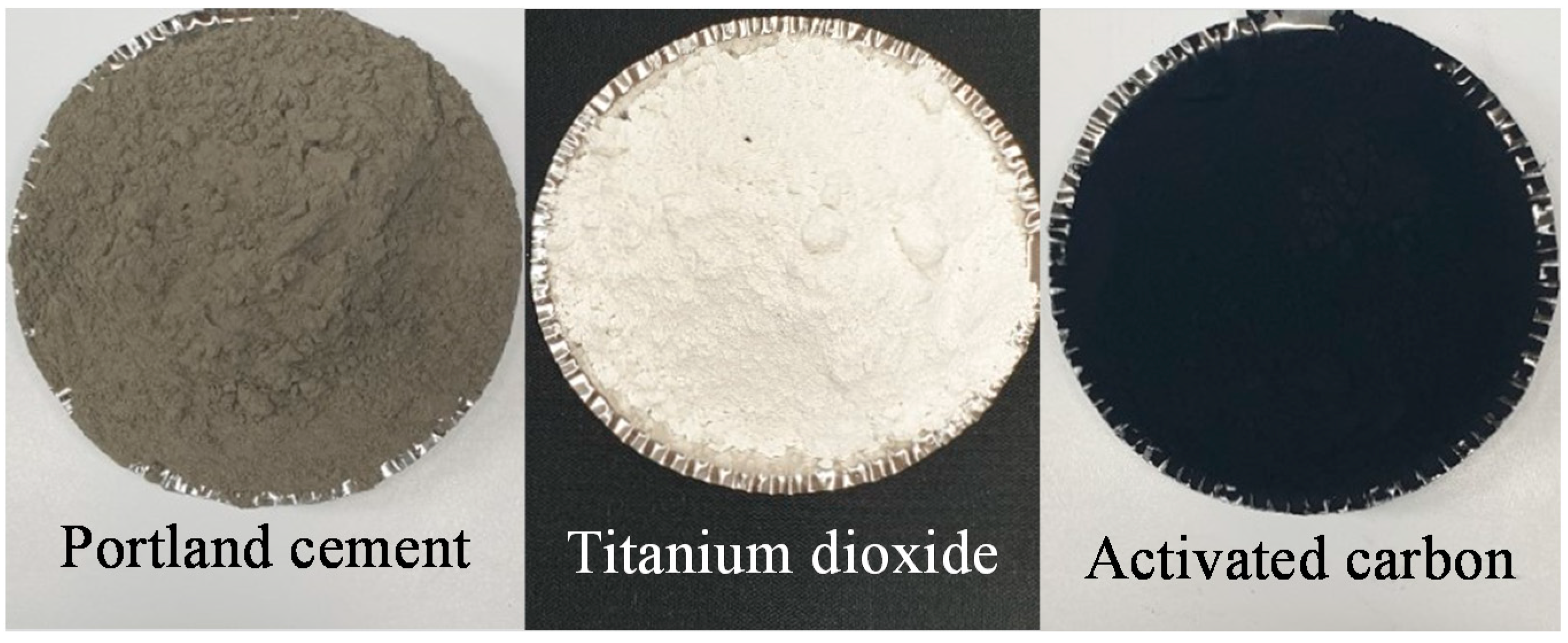
2.1. Specimen Preparation

Two groups of specimens were prepared. The first group (for Dataset I) was used to develop the machine learning model, and the second group (for Dataset II) was used to verify the machine learning model.

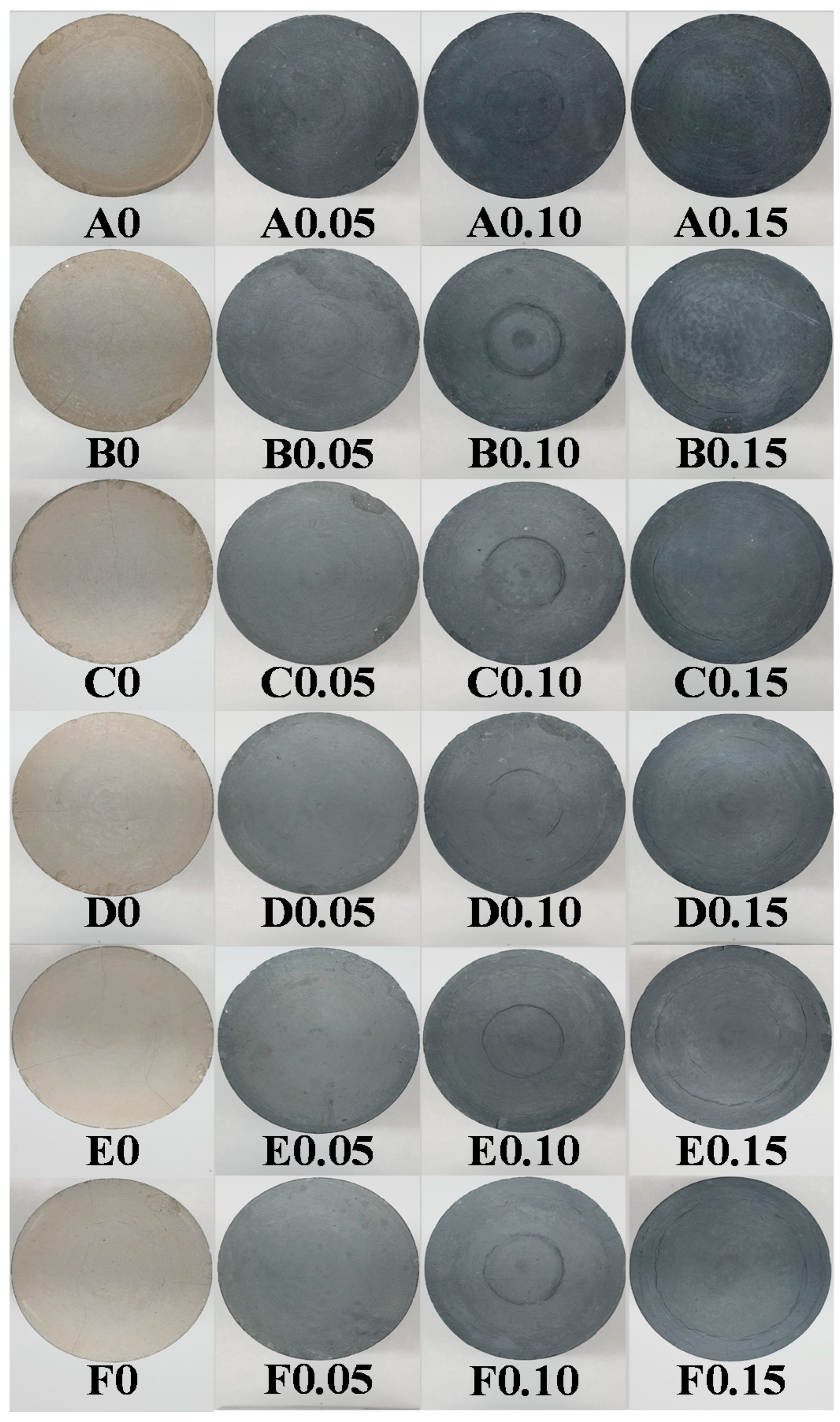
2.1.1. Specimens for Algorithm Development (Dataset I)

Portland cement, TiO₂ (titanium dioxide), and activated carbon were used as basic mixing materials to fabricate the specimens (Figure 1). For the cement material, we used ordinary Portland cement powder with a specific gravity of 3.14, a specific surface area of 4030 cm²/g, and an average particle size of 11.76 μm. For TiO₂, we used the Anatase series with an average particle size of 0.30 μm and purity of 99%. The activated carbon used in this study had a purity of 90% and contained some quartz (SiO₂).

In previous studies, the general mixing ratios of activated carbon for the purpose of reducing harmful substances were 0.01–0.80, relative to the weight of cement, and the mixing ratios of TiO₂ were 0.05–0.40, relative to the weight of cement (e.g., [24,25]). In this study, the specimens for algorithm development were fabricated with activated carbon and TiO₂ mixing ratios of 0–0.15 and 0–0.25, respectively, with reference to the mixing ratios of previous studies.

Table 1. Test cases for algorithm development.

Specimen #	Mixing Ratio
	Activated Carbon (AC)	Titanium Dioxide (TiO2)
A0	0	0
A0.05	0.05	0
A0.10	0.10	0
A0.15	0.15	0
B0	0	0.05
B0.05	0.05	0.05
B0.10	0.10	0.05
B0.15	0.15	0.05
C0	0	0.10
C0.05	0.05	0.10
C0.10	0.10	0.10
C0.15	0.15	0.10
D0	0	0.15
D0.05	0.05	0.15
D0.10	0.10	0.15
D0.15	0.15	0.15
E0	0	0.20
E0.05	0.05	0.20
E0.10	0.10	0.20
E0.15	0.15	0.20
F0	0	0.25
F0.05	0.05	0.25
F0.10	0.10	0.25
F0.15	0.15	0.25

presents the 24 mixing cases for the concrete specimens. The water/cement ratio was fixed at 0.5 (130 g/260 g). Tap water was used (electrical resistivity: 36 Ω∙m). The mixing ratios of TiO₂ relative to the cement weight (260 g) were set as 0, 0.05, 0.10, 0.15, 0.20, and 0.25. Meanwhile, the mixing ratios of activated carbon relative to the cement weight were set as 0, 0.05, 0.10, and 0.15. The TiO₂ mixing ratios of 0, 0.05, 0.10, 0.15, 0.20, and 0.25 are denoted by A, B, C, D, E, and F, respectively, whereas the activated carbon mixing ratios are indicated by numbers (0, 0.05, 0.10, 0.15) following the alphabet index (A, B, C, D, E, F).

The specimens were cured for 14 days in a cylindrical mold with a diameter of 50 mm and a height of 100 mm. During the curing process, the specimens were sealed to prevent moisture evaporation. The laboratory environmental conditions during the curing process were maintained at a temperature of 22.8 ± 0.3 °C and a humidity of 71.5 ± 7.0%. After curing, the measurement surface of the specimen was polished to ensure uniform surface quality (Figure 2).

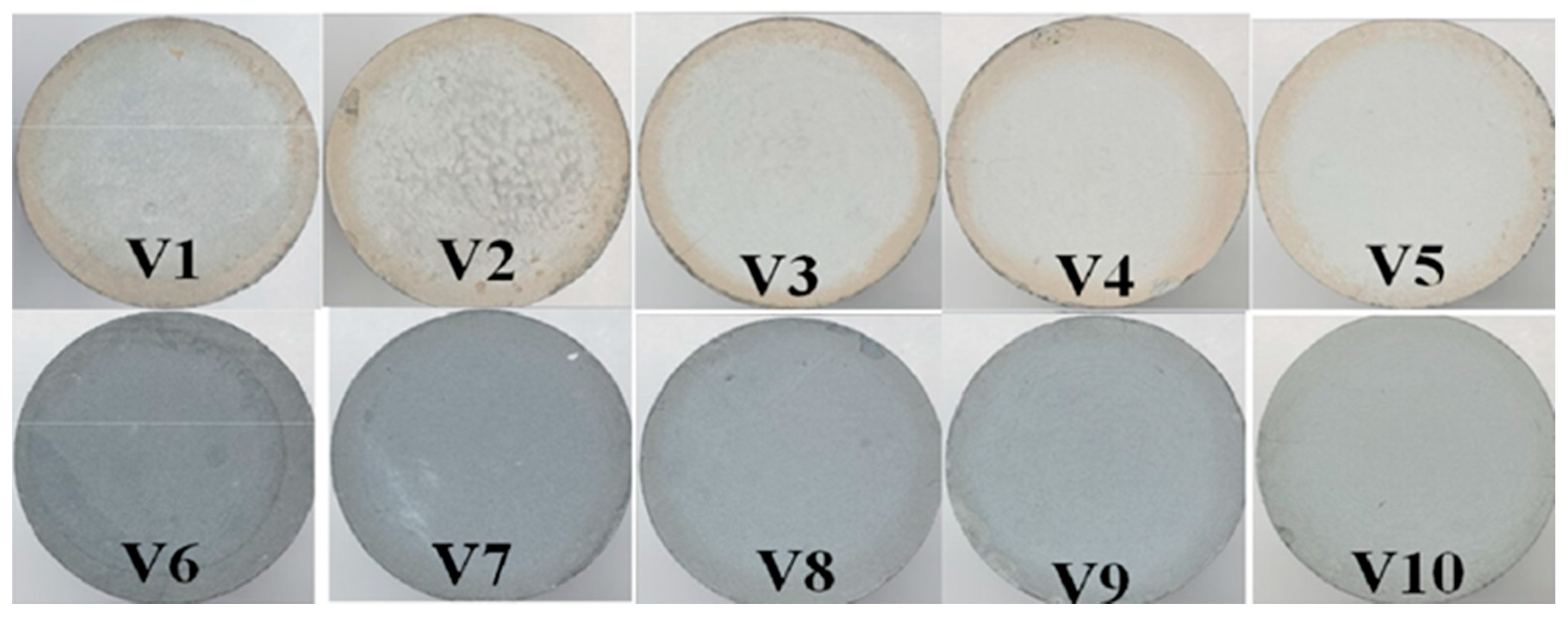
2.1.2. Specimens for Algorithm Verification (Dataset II)

To verify the capability of the machine learning algorithm to evaluate TiO₂ concentration, additional specimens were prepared after the machine learning algorithm was developed.

Table 2. Test cases for algorithm verification.

Specimen #	Cement (g)	Water (g)	Mixing Ratio
			Activated Carbon (AC)	Titanium Dioxide (TiO2)
V1	260	130	0	0.03
V2	260	130	0	0.08
V3	260	130	0	0.13
V4	260	130	0	0.18
V5	260	130	0	0.23
V6	260	130	0.05	0.03
V7	260	130	0.05	0.08
V8	260	130	0.05	0.13
V9	260	130	0.05	0.18
V10	260	130	0.05	0.23

presents the mixing cases for the verification cement specimens. The water/cement ratio was kept constant at 0.5. The mixing ratios of TiO₂ to the cement weight were 0.03, 0.08, 0.13, 0.18, and 0.23, whereas the mixing ratios of activated carbon to the cement weight were 0 and 0.5.

The cement specimens were cured in the laboratory for 14 days. During the curing process, the specimens were sealed to prevent moisture evaporation. The temperature and humidity were maintained at 20.5 ± 0.6 °C and 61.9 ± 2.0%, respectively. After curing, the measurement surfaces of the specimens were again polished using abrasive sandpaper. Figure 3 shows the surfaces of the cured specimens for algorithm verification.

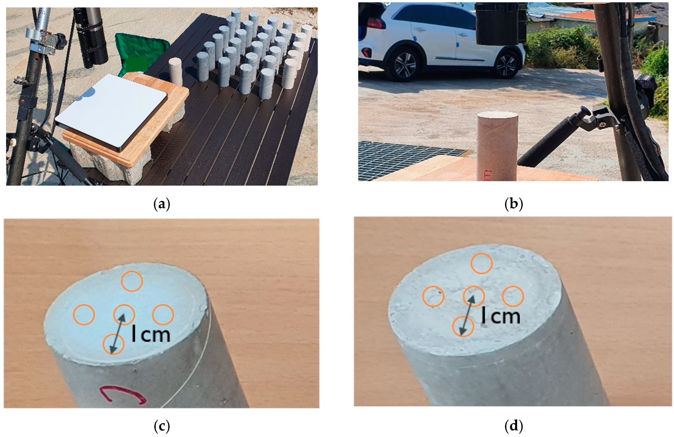
2.2. Measurement of Surface Reflectance with a Hyperspectral Spectroradiometer

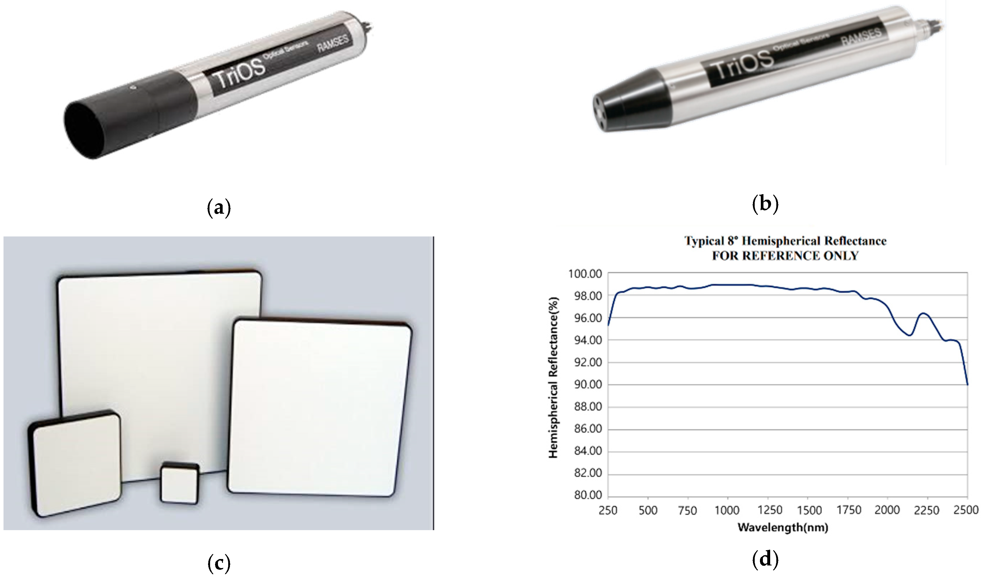
2.2.1. Hyperspectral Sensor and Reflectance

In this study, TriOS RAMSES was used to measure the hyperspectral radiance and irradiance of the samples. The RAMSES system consists of two independent sensors: RAMSES ARC-VIS for radiance and RAMSES ACC-VIS for irradiance (Figure 4). The system is capable of measuring radiance and irradiance in the wavelength range of 320–950 nm, with 3.3 nm spectral resolution. The hyperspectral reflectance ${\rho }_{sample}$ of a sample is then calculated as follows:

$${\rho }_{sample}=\frac{\pi L_{sample}}{E},$$

(1)

where $L_{sample}$ denotes the upwelling radiance reflected from the samples and $E$ denotes the downward irradiance incident on the samples. The ARC-VIS and ACC-VIS sensors directly measure $L_{sample}$ and $E$, respectively. Independent of ACC-VIS for irradiance measurement, a Spectralon white reference panel was also used to measure irradiance with the radiance sensor (Figure 4c). The irradiance measurement with the white reference ($E_{white}$) is calculated as follows:

$$E_{white}=\frac{\pi L_{white}}{{\rho }_{white}},$$

(2)

where $L_{white}$ is the upwelling radiance from the white reference and ${\rho }_{white}$ is the reflectance of the white panel. The reflectance of the Spectralon white panel was almost 99% in the valid wavelength range. Detailed reflectance information can be found in the manual.

2.2.2. Measurement Protocol

Both the radiance and irradiance sensors were positioned to be vertical but in opposite directions: downward for the radiance sensor and upward for the irradiance sensor. The samples were placed horizontally in an open space in such a way that no objects blocked the upper hemisphere of the samples (Figure 5). The distance between the sample and the radiance sensor was maintained at 30 cm. To account for the surface variability, a total of 30 measurements were taken for each sample. Measurements were conducted three times for each of five locations on the surface, and the process was repeated for both faces of the column (top and bottom). The center location of the specimen face was identified first, and four locations were determined at a distance of 1 cm from the center in four directions: up, down, left, and right. The azimuth of the sensor was controlled so that the sensor did not cast a shadow on the samples, nor the center part of the reference panel. The reasoning behind this replication of measurements is mainly because it is extremely difficult to obtain a homogeneous TiO₂ concentration in the sample, both horizontally and vertically throughout the core. The measurement uncertainty is eventually taken into account in the uncertainty of the final estimation algorithm, but this replication was expected to reduce the bias from a small number of samples.

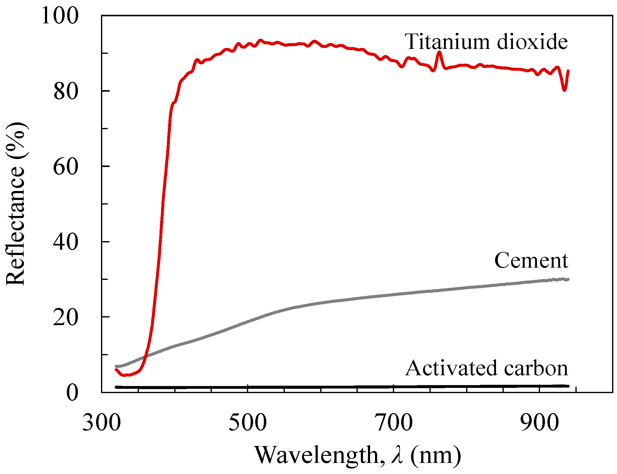
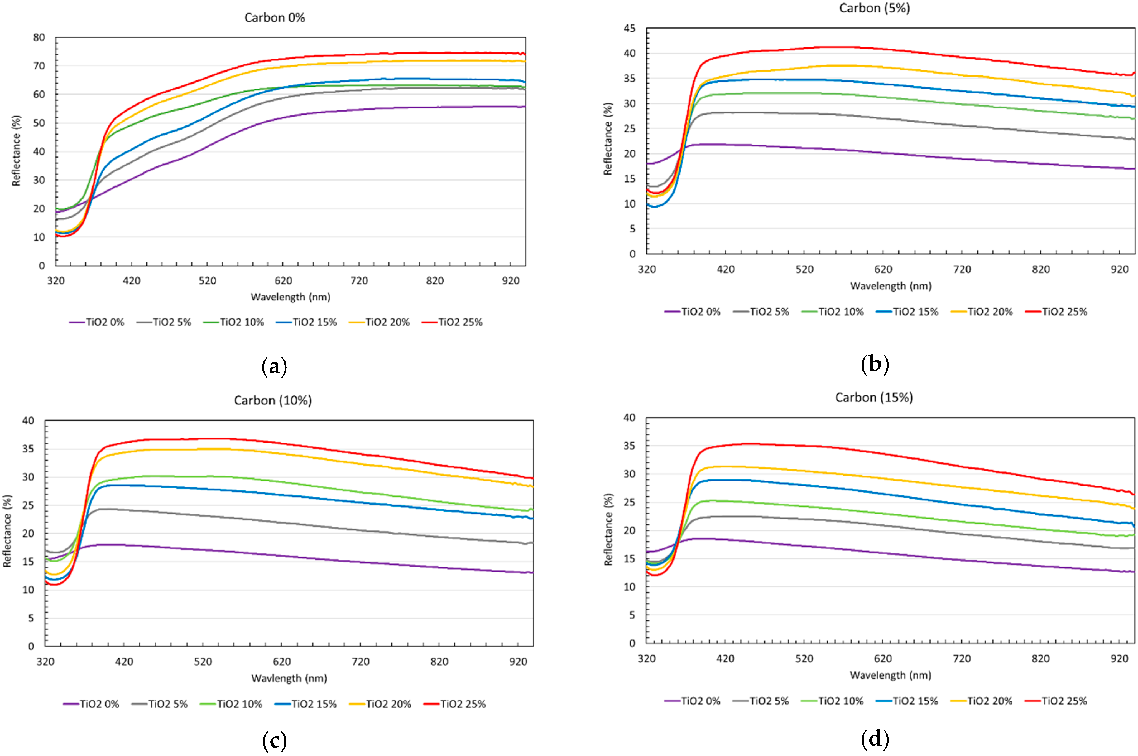
2.3. Spectral Reflectance of Raw and Mixed Materials

Figure 6 presents the reflectance spectrum of the three raw materials (powder type). Consistent with naked-eye observations, TiO₂ had the highest level of reflectance among the three materials and activated carbon had the lowest. A notable reflectance characteristic of TiO₂ is the dramatic reduction in reflectance in the UV spectral range (300–400 nm), where the reflectance decreases from 80%–95% in the visible range to 10% at around 320 nm. Cement exhibits gradually increasing reflectance by wavelength with the reflectance reaching almost 30% at the near-infrared range, around 900 nm. Carbon exhibited a reflectance in the range of 1%–2% across the entire wavelength range tested.

Figure 7 presents the reflectance curves of the specimens for four carbon levels: (a) 0%, (b) 5%, (c) 10%, and (d) 15%. Furthermore, each subfigure contains several reflectance curves corresponding to the various TiO₂ concentrations (0%, 5%, 10%, 15%, 20%, and 25%). Each reflectance curve in Figure 7 represents the mean of 15 measurements conducted on a specific face of the specimen. Across all subfigures, the overall reflectance level increased as the TiO₂ concentration increased, whereas the reflectance decreased as the carbon level increased. This is unsurprising as the reflectance of pure TiO₂ is significantly higher than that of both the base cementitious material and carbon. Furthermore, as the carbon level increased (from (a) to (d)), the reflectance level of the highest curve decreased. However, it is noteworthy that a sharp decrease in reflectance was observed at around 350 nm for all curves. Here, the depth of the valley was deeper for higher TiO₂ concentrations.

Figure 8 presents scatter plots of TiO₂ concentration (%) versus NDTI for different carbon levels. Given a constant NDTI value, the overall TiO₂ concentrations were higher for higher carbon levels. This is because the overall reflectance level decreases with more carbon contained in the samples. Therefore, the estimation of TiO₂ concentration using NDTI requires adjustments according to carbon level. A regression with the quadratic polynomial reveals that a nonlinear relation can be established with a high correlation between TiO₂ concentration and NDTI when the carbon content is fixed or known a priori. Since the carbon content acts as a reflectance reducer, NDTI—which is the measure of the reflectance dip—decreases as carbon contents increase. For example, for the same TiO₂ concentration of 25%, the NDTI values corresponding to the carbon levels of 0%, 5%, 10%, and 15% are approximately 0.60, 0.54, 0.46, and 0.40, respectively. The correlation is high, except in the case of a carbon level of 5%, which was close to one.

While NDTI serves as an effective indicator of TiO₂ concentration, it has limitations in direct use for the estimation of TiO₂ concentration when carbon exists in the sample. As shown in Figure 8, the NDTI–TiO₂ relationship is affected by the level of co-existing carbon in each sample; thus, it is necessary to identify the carbon level before using this relationship.

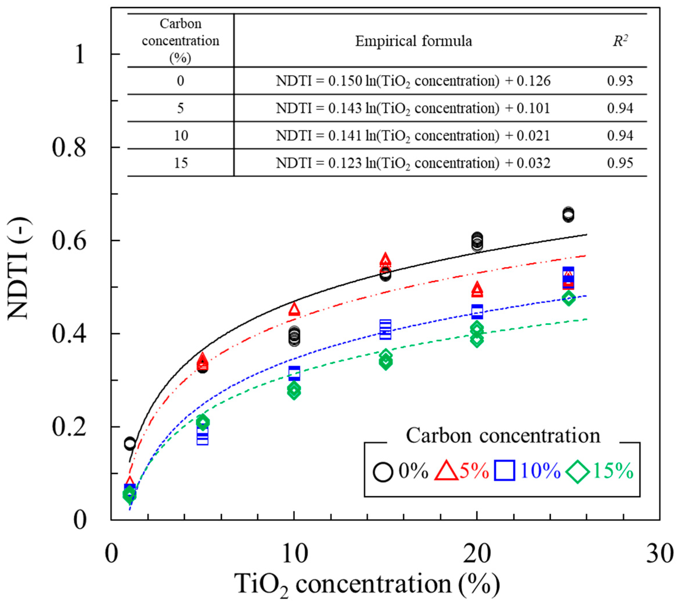
2.4. Normalized Difference TiO₂ Index (NDTI)

As a means to quantify the abundance of TiO₂ in the specimen, the normalized difference TiO₂ index (NDTI) was suggested based on differences in reflectance between the UV and blue spectral regions. As shown in Figure 9, the existence of TiO₂ results in absorption in the UV spectrum, which leads to a reduction in UV reflectance. The reflectance spectrum of the samples, which had varying amounts of TiO₂, revealed that the reduction in UV reflectance became greater as the TiO₂ concentration increased, suggesting a potential linear or nonlinear correlation between UV reflectance reduction and TiO₂ abundance. The proposed NDTI is expressed as follows:

$$\mathrm{NDTI}=\frac{{\rho }_{blue}-{\rho }_{UV}}{{\rho }_{blue}+{\rho }_{UV}} ,$$

(3)

where ${\rho }_{blue}$ and ${\rho }_{UV}$ represent reflectance at the spectral wavelengths of blue and near-infrared light, respectively. In this study, the wavelengths for the UV and blue spectra were selected as ${\mathsf{\lambda }}_{\mathrm{UV}}=338\mathrm{nm}$, and ${\mathsf{\lambda }}_{\mathrm{blue}}=400\mathrm{nm}$, respectively, based on the second derivative of the reflectance curve with a TiO₂ concentration of 15% (Figure 9). This result indicated that zero-crossings of the second derivative occur near 338 nm and 400 nm, indicating that the curve starts to demonstrate reflectance changes by TiO₂ at these points.

2.5. Machine Learning for the Estimation of TiO₂ Concentration

2.5.1. Machine Learning Algorithms

In this study, we constructed five machine-learning-based algorithms to directly estimate TiO₂ relationships from radiometric measurements of the surface. The algorithms were tested with independent samples with varying TiO₂ and carbon contents. The five algorithms included ridge regression (RR), Lasso regression (LR), support vector regression (SVR), random forest (RF), and extreme gradient boosting (XGBoost).

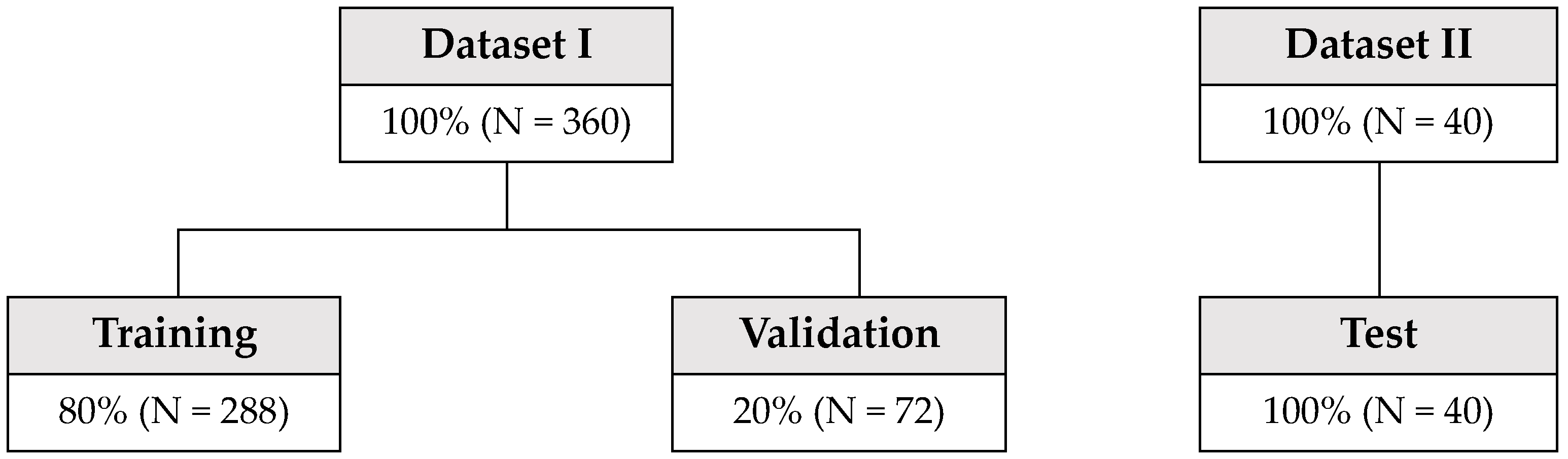
2.5.2. Dataset for Algorithm Development (Dataset I) and Test (Dataset II)

Algorithm development of all machine learning methods was performed with Dataset I, which consisted of 360 reflectance data points (Figure 10). The predictors of machine learning were reflectance data in the wavelength range of 320 to 939 nm, and about 620 were used. To determine the model parameters of each algorithm, we employed the five-fold bagging scheme. First, Dataset I was randomly divided into five bags, each of which contained 20% of the entire data. Data samples from four bags are used for the training data, and the data from the remaining bag are used for validation. This process can be repeated five times as we have five choices of validation data. The results from the five runs were used to derive the statistical performance of the algorithms with each validated parameter set.

An optimal parameter set was sought via a greedy grid search for all algorithms. The search range of each parameter was initially selected based on a trial-and-error approach, and the parameter set with the best performance in the validated range was identified as the optimal parameter set for the corresponding algorithm. The parameter ranges used for tuning are presented in

Table 3. Parameter values of machine learning algorithms.

Machine Learning Algorithm	Parameters	Value Range	Value
Ridge regression	λ	1~0.00001	0.0001
Lasso regression	λ	1~0.00001	0.0005
Support vector regression	Kernel	Linear, Poly, RBF, Sigmoid	RBF
	gamma	1~0.0001	1
	C	1~0.0001	1
Random forest	bootstrap	True, False	True
	max_depth	100~10, None	50
	max_features	Auto, Sqrt	Sqrt
	min_samples_leaf	20~1	10
	min_samples_split	20~1	10
	n_estimators	5000~100	1000
XGBoost	booster	gbtree, gblinear	gbtree
	learning_rate	1~0.001	0.001
	max_depth	10~1	8
	subsample	1~0.1	1
	max_features	1~0.1	0.5
	min_child_weight	20~1	15
	colsample_bytree	1~0.1	0.6
	n_estimators	10,000~1000	5000
	Early Stopping	300	300

, with the optimal parameter values in the right column. Each machine learning algorithm was then applied with its optimal parameter set to the independent test dataset (Dataset II) to derive a generalized estimation of the performance of the algorithm.

3. Results and Analysis

3.1. Performance of the Machine Learning Methods

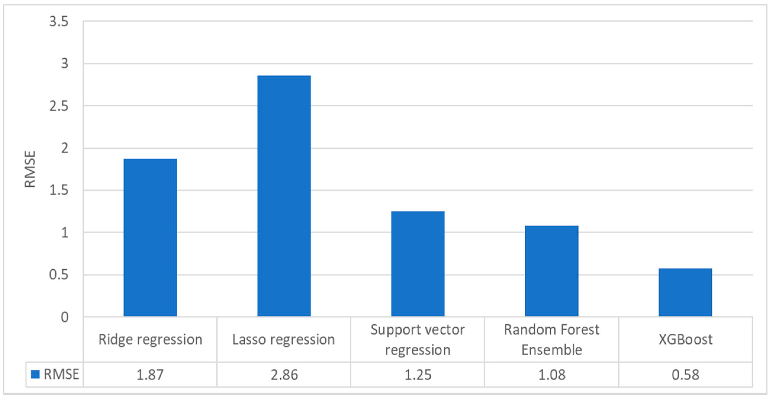
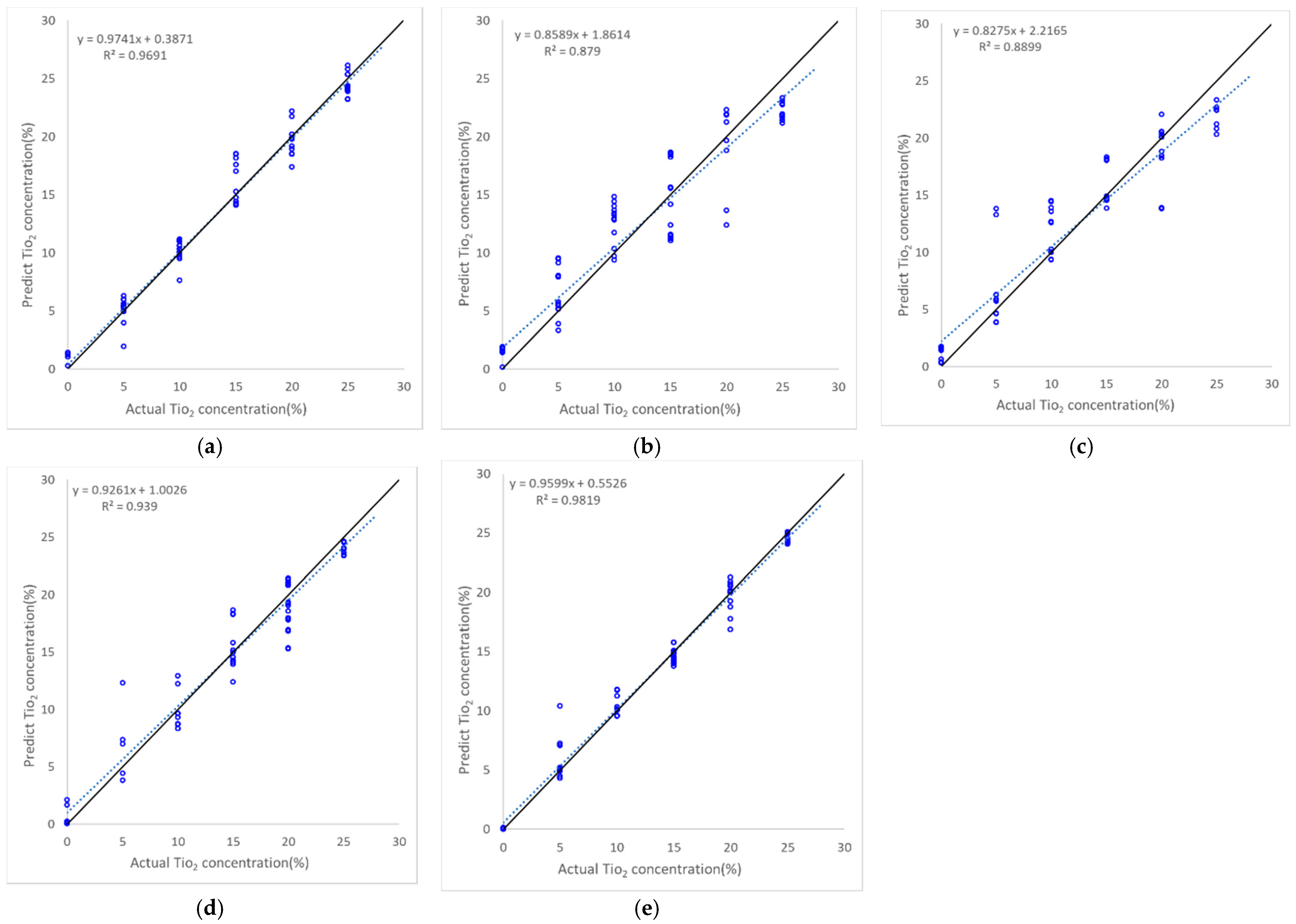
3.1.1. Training Accuracy

Figure 11 presents the root-mean-square-error of the tested methods. Note that the unit (i.e., percent) is from the unit of the independent variable—namely, the TiO₂ concentration itself—and does not indicate the relative accuracy as a ratio to any other reference value, such as the mean of the estimates. Among the five methods, XGBoost performed the best, producing an RMSE of 0.6%, whereas the worst-performing model was Lasso regression, as shown by its RMSE of approximately 3%. Considering the tested TiO₂ concentrations, which ranged from 0% to 25%, models with an RMSE of less than 1% can be regarded as having high estimation precision.

Figure 12 presents scatter plots between the true and estimated TiO₂ concentrations, through which the performance according to the TiO₂ range can be further analyzed. Among the five tested algorithms, XGBoost performed the best with an RMSE of around 0.6%, whereas Lasso regression had the worst performance with an RMSE of around 2.9%. There is no clear dependency between the accuracy and the TiO₂ level in all methods except for Lasso regression, which exhibited moderate errors for the specimen with 20% TiO₂. The main cause of deviations of data points from the 1:1 line seen in all figures was considered to be the varying carbon contents of the specimens. Additionally, many other sources of measurement uncertainty (e.g., inhomogeneity of the surface) exist.

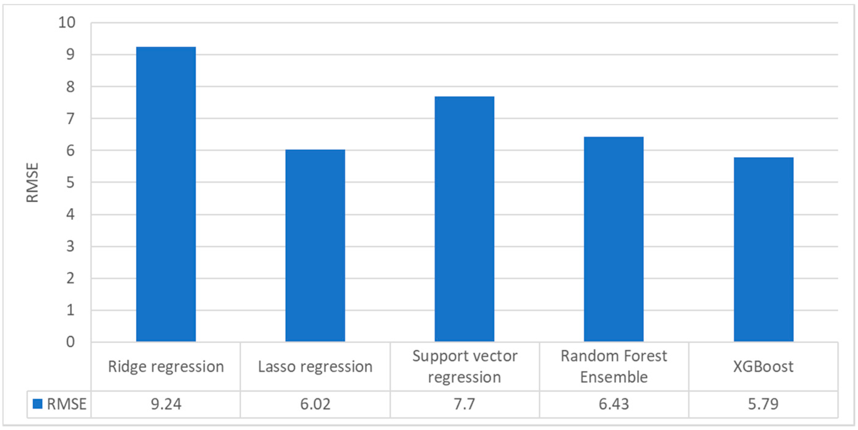
3.1.2. Test Accuracy

To derive more generalized results in terms of the performance of the five machine learning algorithms, the trained algorithms were applied to the independent test data (Dataset II). Figure 13 reveals that the results from the test data were generally worse than those obtained using the validation dataset, regardless of the method. This is typical of the training and test process of machine learning approaches. In terms of uncertainty, XGBoost again produced the best RMSE (around 6%), whereas the ridge regression method exhibited the worst result with an RMSE of approximately 9%. The other methods exhibited RMSE values of around 6%–8%.

The scatter plot of each method provides additional insights into the performance of the model that cannot be represented by RMSE (Figure 14). In contrast to the performance as analyzed by RMSE, where Ridge regression had the lowest performance among the five methods, in terms of correlation, the Ridge regression exhibited the best R² (around 0.93). However, this method exhibited large TiO₂ biases for concentrations greater than 10. Lasso regression had the most stable performance with an RMSE of around 6% and an R² of approximately 0.8, despite the consistent overestimation observed throughout the entire range. XGBoost exhibited a similar RMSE level to Lasso but, as represented by its R² score, the scatter was greater than that of the Lasso regression method. Lastly, support vector regression produced the lowest R² (<0.1); however, its RMSE result of around 8% is not overly poor when compared with the other methods. This indicates that RMSE alone does not represent the performance of the method.

4. Discussion: Limitations and Strengths

This study validates the feasibility of TiO₂ estimation using the proposed machine learning model for cementitious specimens. Although the results demonstrate the robustness of the suggested model (Lasso regression), the following limitations apply: A certain portion of the uncertainty in the estimation is driven by the heterogeneity of specimen surfaces, which include locational differences on a single specimen surface in addition to differences between different specimens. Ideally, the specimen surface should be fabricated and maintained perfectly uniform in terms of both the base cementitious material and the TiO₂ concentration with no locational dependency; however, this is difficult to realize practically considering the curing process. In addition, downward gravitational pressure is another factor that increases the heterogeneity of the surface as it causes the cross sections to vary according to the specimen height. As this study did not perform an analysis of the quantification of such spatial heterogeneity, it is difficult to calculate the degree to which specimen heterogeneity contributed to the estimation uncertainty.

One downside of using a machine learning approach for estimation work is that it is difficult to explain the causes of differences between the training and test results unless a specific experimental design is not contemplated via, for example, the use of explainable machine learning approaches. The process of specimen fabrication was maintained strictly identical for both Dataset I and Dataset II by using the same conditions (e.g., curing humidity and temperature). However, certain uncontrollable environmental variables would have affected the curing process (e.g., an uneven blend distribution of the specimen). The performance differences between Dataset I and Dataset II were likely to have been affected by such variations.

The strength of this study is that, unlike a previous study [23], the proposed model can estimate TiO₂ concentration across a very wide concentration range (up to 30%) and in cases of co-existence with activated carbon, which is often the case in the field. Another important aspect of the proposed algorithms is its robustness in interpreting the estimation results. A robust algorithm should have low sensitivity for such uncontrollable and unpredictable, yet commonly encountered, factors. Our results indicated that Lasso regression has the highest robustness for TiO₂ estimation. Since performance in a training process does not represent the actual performance on independent data, it is not necessary to explain why the performance ranking in the training process was inverted compared with that of the test step.

5. Conclusions and Suggestions

This study explored spectral reflectance characteristics according to the TiO₂ and activated carbon ratios in concrete specimens using a hyperspectral sensor. Based on the experimental database, this study demonstrates the feasibility of machine learning algorithms to estimate the remaining TiO₂ and activated carbon ratios for concrete structures. The main findings are as follows:

• TiO₂ powder has a high level of reflectance (around 80%–95%) that is dramatically reduced in the UV spectral range (300–400 nm). On the other hand, activated carbon powder has very low reflectance, as demonstrated by its approximate 1%–2% reflectance over the entire wavelength range tested.
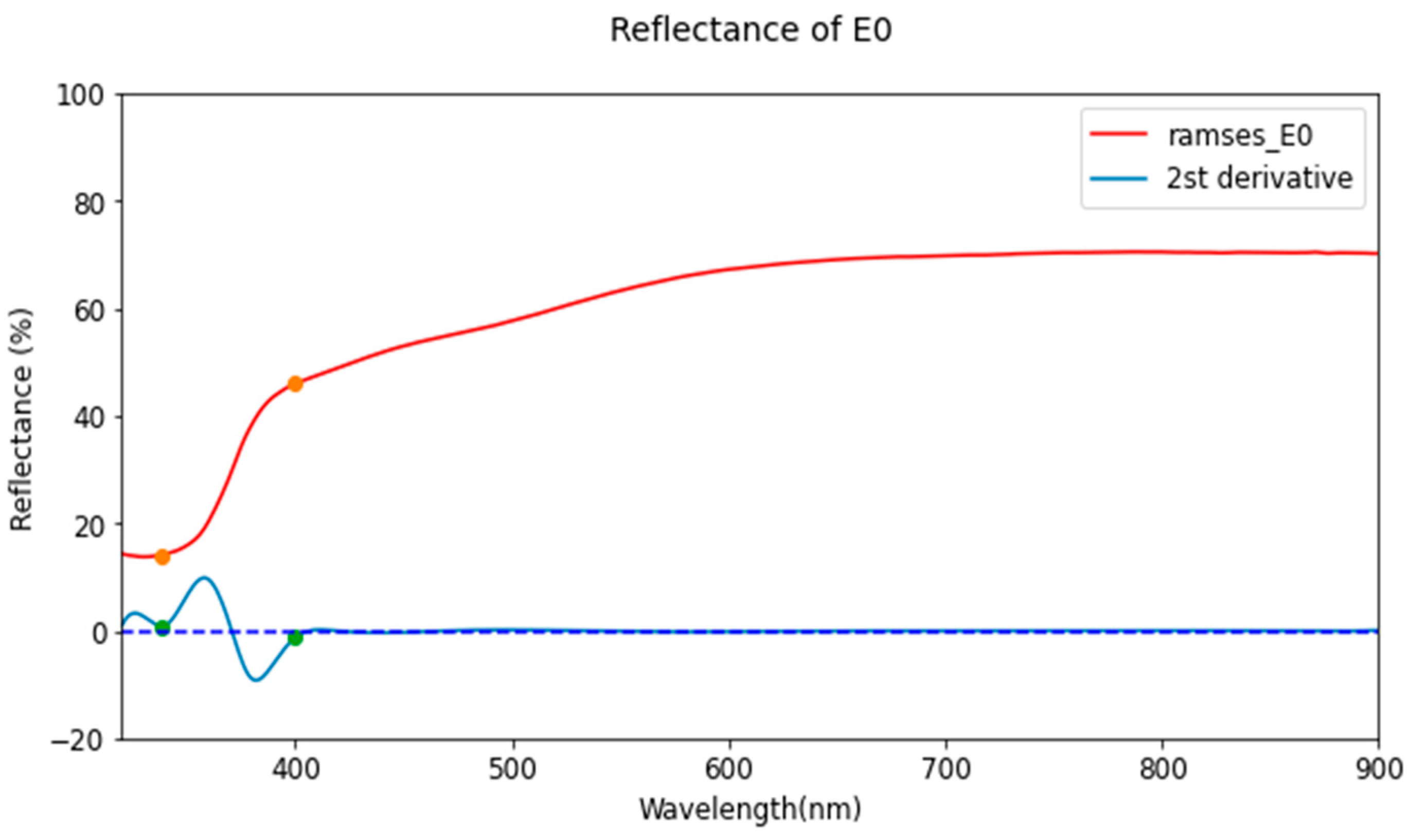
• The overall reflectance level increased with increasing TiO₂ concentration and decreasing carbon ratio in the concrete specimens. The reflectance curves revealed a common sharp decrease in reflectance at around 350 nm for all specimens; specifically, the depth of the valley was deeper for higher TiO₂ concentrations.
• The normalized difference TiO₂ index (NDTI) was suggested in this study based on reflectance differences in the UV and blue spectral regions. Based on the experimental results, the regression with the quadratic polynomial shows a good relationship between TiO₂ concentration and NDTI when the carbon ratio is fixed.
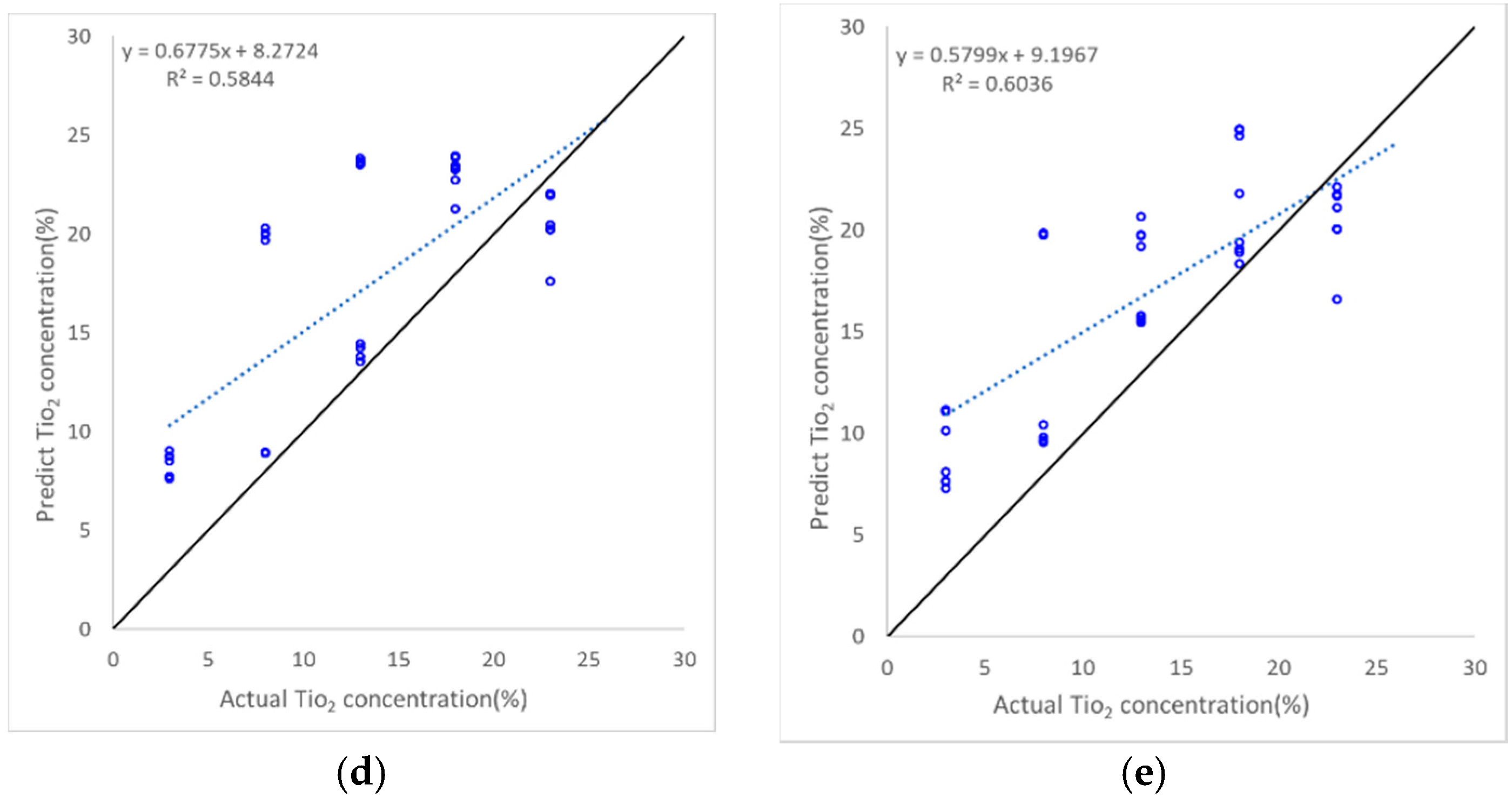
• Performance analysis of the machine learning methods considered in this study revealed that most methods worked well with the training/validation data (Dataset I). However, when applied to the test data (Dataset II), Lasso regression was the most robust method; it was possible to estimate the TiO₂ concentration with 6% RMSE and a correlation level of 0.8.
• The suggested robust machine learning approach can be adjusted and expanded to field applications by, for example, employing camera-type hyperspectral sensors that can estimate TiO₂ using images of wide areas.

References

1. European Environmental Agency (EEA) Reports. Available online: https://www.eea.europa.eu/themes/air/health-impacts-of-air-pollution (accessed on 31 December 2021).
2. Kim, Y.P. Research and Policy Directions against Ambient Fine Particles. J. Korean Soc. Atmos. Environ. 2017, 33, 191–204. [Google Scholar] [CrossRef]
3. Kang, C.M.; Park, S.G.; Sunwoo, Y.; Kang, B.W.; Lee, H.S. Respiratory health effects of fine particles (PM2.5) in Seoul. J. Korean Soc. Atmos. Environ. 2006, 22, 554–563. [Google Scholar]
4. Ângelo, J.; Andrade, L.; Madeira, L.M.; Mendes, A. An overview of photocatalysis phenomena applied to NOx abatement. J. Environ. Manag. 2013, 129, 522–539. [Google Scholar] [CrossRef]
5. Beeldens, A. An Environmental Friendly Solution for Air Purification and Self-Cleaning Effect: The Application of TiO2 as Photocatalyst in Concrete; Transport Research Arena Europe-TRA: Göteborg, Sweden, 2006; pp. 12–16. [Google Scholar]
6. Boonen, E.; Beeldens, A. Recent photocatalytic applications for air purification in Belgium. Coatings 2014, 4, 553–573. [Google Scholar] [CrossRef] [Green Version]
7. Cárdenas, C.; Tobón, J.I.; García, C.; Vila, J. Functionalized building materials: Photocatalytic abatement of NOx by cement pastes blended with TiO2 nanoparticles. Constr. Build. Mater. 2012, 36, 820–825. [Google Scholar] [CrossRef]
8. Lee, B.Y.; Jayapalan, A.R.; Bergin, M.H.; Kurtis, K.E. Photocatalytic cement exposed to nitrogen oxides: Effect of oxidation and binding. Cem. Concr. Res. 2014, 60, 30–36. [Google Scholar] [CrossRef]
9. Pérez-Nicolás, M.; Balbuena, J.; Cruz-Yusta, M.; Sánchez, L.; Navarro-Blasco, I.; Fernández, J.M.; Alvarez, J.I. Photocatalytic NOx abatement by calcium aluminate cements modified with TiO2: Improved NO2 conversion. Cem. Concr. Res. 2015, 70, 67–76. [Google Scholar] [CrossRef] [Green Version]
10. Guerrini, G.L. Photocatalytic performances in a city tunnel in Rome: NOx monitoring results. Constr. Build. Mater. 2012, 27, 165–175. [Google Scholar] [CrossRef]
11. Folli, A.; Strøm, M.; Madsen, T.P.; Henriksen, T.; Lang, J.; Emenius, J.; Klevebrant, T.; Nilsson, Å. Field study of air purifying paving elements containing TiO2. Atmos. Environ. 2015, 107, 44–51. [Google Scholar] [CrossRef]
12. Kim, Y.K.; Hong, S.J.; Kim, H.B.; Lee, S.W. Evaluation of in-situ NOx removal efficiency of photocatalytic concrete in expressways. KSCE J. Civ. Eng. 2018, 22, 2274–2280. [Google Scholar] [CrossRef]
13. Horgnies, M.; Dubois-Brugger, I.; Gartner, E.M. NOx de-pollution by hardened concrete and the influence of activated charcoal additions. Cem. Concr. Res. 2012, 42, 1348–1355. [Google Scholar] [CrossRef]
14. Horgnies, M.; Serre, F.; Dubois-Brugger, I.; Gartner, E. NOx De-pollution using activated charcoal concrete—From laboratory experiments to tests with prototype garages. Cem. Concr. Res. 2014, 42, 1348–1355. [Google Scholar] [CrossRef]
15. Di Tommaso, M.; Bordonzotti, I. NOx adsorption, fire resistance and CO2 sequestration of high performance, high durability concrete containing activated carbon. In Proceedings of the Second International Conference on Concrete Sustainability, Madrid, Spain, 13–15 June 2016; Volume 192, pp. 1–12. [Google Scholar]
16. Russell, H.S.; Frederickson, L.B.; Hertel, O.; Ellermann, T.; Jensen, S.S. A Review of Photocatalytic Materials for Urban NOx Remediation. Catalysts 2021, 11, 675. [Google Scholar] [CrossRef]
17. Chen, M.; Chu, J.W. NOx photocatalytic degradation on active concrete road surface—From experiment to real-scale application. J. Clean. Prod. 2011, 19, 1266–1272. [Google Scholar] [CrossRef]
18. De Melo, J.V.S.; Trichês, G.; Gleize, P.J.P.; Villena, J. Development and evaluation of the efficiency of photocatalytic pavement blocks in the laboratory and after one year in the field. Constr. Build. Mater. 2012, 37, 310–319. [Google Scholar] [CrossRef]
19. Ballari, M.M.; Brouwers, H.J.H. Full scale demonstration of air-purifying pavement. J. Hazard. Mater. 2013, 254, 406–414. [Google Scholar] [CrossRef] [PubMed] [Green Version]
20. Osborn, D.; Hassan, M.; Asadi, S.; White, J.R. Durability quantification of TiO2 surface coating on concrete and asphalt pavements. J. Mater. Civ. Eng. 2014, 26, 331–337. [Google Scholar] [CrossRef]
21. Lee, S.W.; Ahn, H.R.; Kim, K.S.; Kim, Y.K. Applicability of TiO2 Penetration Method to Reduce Particulate Matter Precursor for Hardened Concrete Road Structure. Sustainability 2021, 13, 3433. [Google Scholar] [CrossRef]
22. Luo, G.; Liu, H.; Li, W.; Lyu, X. Automobile exhaust removal performance of pervious concrete with nano TiO2 under photocatalysis. Nanomaterials 2020, 10, 2088. [Google Scholar] [CrossRef]
23. Costanzo, A.; Ebolese, D.; Ruffolo, S.A.; Falcone, S.; La Piana, C.; La Russa, M.F.; Musacchio, M.; Buongiorno, M.F. Detection of the TiO2 Concentration in the Protective Coatings for the Cultural Heritage by Means of Hyperspectral Data. Sustainability 2021, 13, 92. [Google Scholar] [CrossRef]
24. Ra, D.G.; Lee, G.D.; Jeong, S.C.; Kim, Y.G. Assesment of strength property and photocatalytic activity of TiO2-added mortar. J. Korean Soc. Environ. Eng. 2003, 25, 1499–1503. [Google Scholar]
25. Zhang, Y.; Wang, Y.; Yang, C.; Li, G.; Yan, H. Study on the reduction of radon exhalation rates of concrete with different activated carbon. Key Eng. Mater. 2017, 726, 558–563. [Google Scholar] [CrossRef]
Figure 1. Materials used for the test specimens.
Remotesensing 14 00189 g001
Figure 2. Surfaces of the cured specimens for testing.
Remotesensing 14 00189 g002
Figure 3. Surfaces of cured specimens for algorithm verification.
Remotesensing 14 00189 g003
Figure 4. (a) RAMSES ARC-VIS, (b) RAMSES ACC-VIS, (c) Spectralon white reference panel, and (d) reflectance of the white reference panel.
Remotesensing 14 00189 g004
Figure 5. Setting of TriOS RAMSES sensors for the sample reflectance measurement (a,b), and the five locations of the measurement points on (c) the top face of the specimen, and (d) the bottom face of the specimen.
Remotesensing 14 00189 g005
Figure 6. Reflectance curves of the raw materials (titanium dioxide, Portland cement, and activated carbon).
Remotesensing 14 00189 g006
Figure 7. Reflectance curves of cementitious base samples with varying TiO2 contents. Each subfigure corresponds to a different carbon level: (a) 0%, (b) 5%, (c) 10%, and (d) 15%.
Remotesensing 14 00189 g007
Figure 8. Scatter plots of TiO2 concentration (%) versus NDTI for different carbon levels.
Remotesensing 14 00189 g008
Figure 9. Hyperspectral reflectance spectra of a sample with a TiO2 concentration of 15%, displayed with the second derivative of the spectra. Two inflection points are observed at around 338 nm and 400 nm where the second derivative equals to zero.
Remotesensing 14 00189 g009
Figure 10. Data arrangement and split scheme for machine learning training/validation (Dataset I) and test (Dataset II).
Remotesensing 14 00189 g010
Figure 11. Bar graphs representing the TiO2 estimation performance of the five machine learning algorithms when applied to the training/validation dataset (Dataset I).
Remotesensing 14 00189 g011
Figure 12. Scatter plots of the TiO2 estimation performance for Dataset I of the five machine learning algorithms; (a) Ridge regression; (b) Lasso regression; (c) Support vector regressor; (d) Random Forest Ensemble; (e) XGBoost. The 1:1 line is in black, and the blue dashed line represents the regression line fitted to actual and predicted TiO2 concentrations.
Remotesensing 14 00189 g012
Figure 13. Bar graph representing the TiO2 estimation performance of the five machine learning algorithms when applied to the test dataset (Dataset II).
Remotesensing 14 00189 g013
Figure 14. Scatter plots of the TiO2 estimation performance for Dataset II of the five machine learning algorithms; (a) Ridge regression; (b) Lasso regression; (c) Support vector regressor; (d) Random Forest Ensemble; (e) XGBoost. The 1:1 line is in black, and the blue dashed line represents the regression line fitted to actual and predicted TiO2 concentrations.
Remotesensing 14 00189 g014aRemotesensing 14 00189 g014b