Graph SLAM-Based 2.5D LIDAR Mapping Module for Autonomous Vehicles

Abstract

This paper proposes a unique Graph SLAM framework to generate precise 2.5D LIDAR maps in an XYZ plane. A node strategy was invented to divide the road into a set of nodes. The LIDAR point clouds are smoothly accumulated in intensity and elevation images in each node. The optimization process is decomposed into applying Graph SLAM on nodes’ intensity images for eliminating the ghosting effects of the road surface in the XY plane. This step ensures true loop-closure events between nodes and precise common area estimations in the real world. Accordingly, another Graph SLAM framework was designed to bring the nodes’ elevation images into the same Z-level by making the altitudinal errors in the common areas as small as possible. A robust cost function is detailed to properly constitute the relationships between nodes and generate the map in the Absolute Coordinate System. The framework is tested against an accurate GNSS/INS-RTK system in a very challenging environment of high buildings, dense trees and longitudinal railway bridges. The experimental results verified the robustness, reliability and efficiency of the proposed framework to generate accurate 2.5D maps with eliminating the relative and global position errors in XY and Z planes. Therefore, the generated maps significantly contribute to increasing the safety of autonomous driving regardless of the road structures and environmental factors.

1. Introduction

Maps are a very important pillar to enable autonomous driving by encoding the real world with good weather factors and environmental conditions. Maps are mainly used to localize vehicles in the XY plane for safely conducting autonomous maneuvers with respect to other road users [1,2]. In the Z plane, the maps are utilized to estimate pitch and roll angles as well as to measure distances to other vehicles [3]. Therefore, the mapping module must generate precise maps in terms of accurately positioning roads in XY-Z planes and integrating the environmental representations at a high definition level.

Tunnels, dense trees, high buildings and railways are considered as challenging road structures that may deflect and obstruct satellite signals even with the use of accurate GNSS/INS-RTK (GIR) systems. This leads to ghosting effects in the XY map domain because of the relative-position errors. The ghosting effects decrease the localization accuracy because of changing the road pattern compared to that encoded in the observation data during the autonomous driving as illustrated in Figure 1a. In the Z plane, the altitudinal relative-position errors change the road slope and create virtual/unreal bumps in the road consistency. Both of these phenomena indicate global-position errors of the map in the Absolute Coordinate System (ACS). Thus, increasing the robustness of the mapping module against challenging environments is a critical demand to globalize autonomous driving safely.

Graph SLAM (GS) is a dominant approach to increase map accuracy in a probabilistic framework. Thrun applied Graph SLAM, showing promising results to enhance the map and trajectory positions [4]. Grisetti then explained the implementation steps in a simpler manner, illustrating experimental results by a small robotics platform [5]. Olson detailed some technical aspects to magnify the utilization level, such as strategizing loop-closure detection, covariance estimation and switchable constraints of GPS modeling [6]. Roh proposed a framework called ISAM to generate maps based on LIDAR 3D point clouds and camera images [7]. The altitudinal features, such as walls and building fronts, are segmented in the point clouds to create a set of polygons. Loop-closure events are detected according to the similarity score between the segmented walls to compensate the localization errors. The walls are decomposed in lines in the Z-direction and a full 3D map is then constructed by incorporating the elevation measurements of the lines. All of these components are integrated into a pose-slam platform to optimize the relationships between the vehicle positions and generate precise maps. Triebel suggested a Graph SLAM approach to generate 3D maps based on dividing, clustering and classifying the point clouds into multilayers [8]. A cloud is divided into a set of fixed-size cells with respect to the height interval. The divided cells are then determined to represent vertical and horizontal structures in the real world. This tactic facilitates the loop-closure detection and improves the matching process between point clouds using iterative closest point (ICP) [9]. As each point cloud is assigned into a robot position, a set of constraints are designed to constitute the relationships between positions in ACS. Finally, an optimization process is applied to optimize the robot trajectory as well as the point cloud distributions in the map domain. Recently, an impressive effort has been demonstrated to apply SLAM based on ground feature extraction in the LIDAR point cloud [10]. The extracted features are then classified into edge and planner groups and used by the Levenberg-Marquardti optimization technique to estimate the vehicle poses in consecutive scans. Another method called LIO-SAM has been proposed to incorporate the estimated motion from an inertial measurement unit with the results of LIDAR scan matching for optimizing the vehicle trajectory [11].

Most SLAM-proposed approaches operate in the point cloud domain [12] and rely on point distribution pattern-based iterative matching strategies to process xyz positions at once. This may reduce the utilization of environmental features to compensate relative position errors due to the LIDAR sparsity. Moreover, wrong matching results might be provided because of changing the distribution patterns, especially in the Z-direction at the revisited areas. In featureless areas and wide road segments, the features in the Z-direction do not play a significant role in enhancing the matching quality as illustrated in Figure 2a. Furthermore, the altitudinal features in urban environments may also negatively affect the matching process. For example, stopped cars at a traffic signal might be registered in a point cloud and prevent the encoding of the real stationary environmental features as shown in Figure 2b. The vehicle may revisit the same traffic signal during the map-data collection with encoding either different patterns of stopped cars or the real stationary environmental features. Consequently, the matching results in both cases to the registered point-cloud in the first visit at the traffic signal will be wrong.

The 2.5D maps are very promising components to power autonomous vehicles because of reducing the storing size, providing dense details, decreasing the data representation and sufficiently enabling real-time processes compared to 3D point cloud maps. In addition, the 2.5D maps provide elevation values that can be used to enable many applications, such as localization [13], pitch and roll angle calculations [3,14] and obstacle distance estimation [15]. Furthermore, it allows the use of map matching models in the image domain [16] instead of point cloud-based registration methods [17,18]. This significantly decreases the mismatching events because of using LIDAR reflectivity compared to the 3D point distribution patterns [19]. This enables a continuous dense representation of environments, reduces the processing time of compensating relative position errors and simplifies the implementation process. However, applying SLAM technologies to generate accurate 2.5D maps using LIDAR elevation and intensity data is still challenging and rarely addressed [20,21,22]. We previously proposed a GS framework to generate precise LIDAR elevation maps in the Z-direction without processing the map in the XY plane [21]. However, the need to use 2.5D maps (elevation and intensity) has significantly emerged to enable many applications, such as 3D localization, pith and roll online calibration, building 3D perception model-based fusion camera and LIDAR data. Hence, we present in this paper a unique GS framework to generate precise 2.5D LIDAR maps emphasizing the robustness and reliability in very challenging environments and road structures.

2. Key Solution and Proposed Strategy

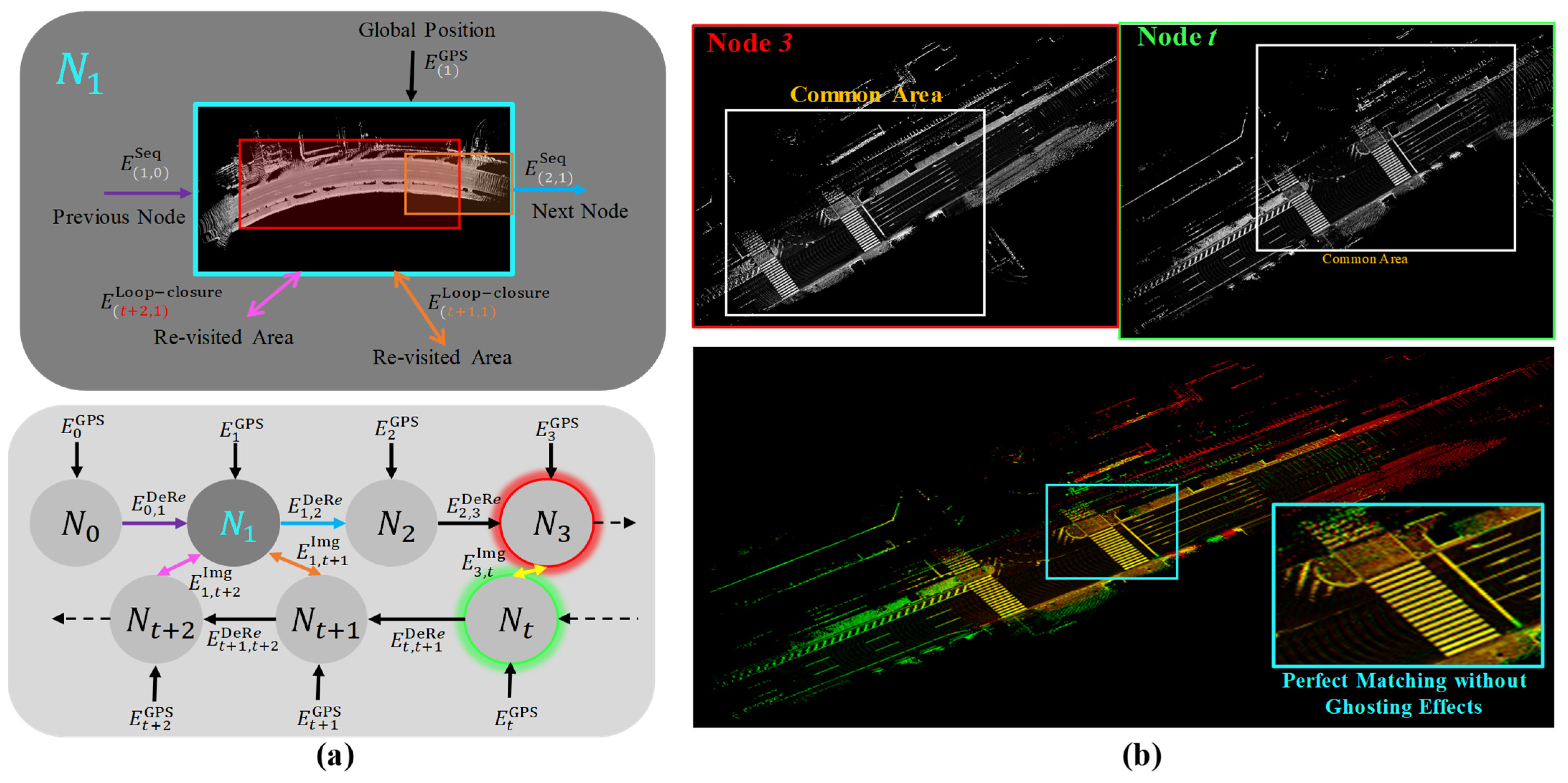
The most important pillars to obtain reliable results by SLAM are the utilization strategy of the environmental features to compensate the relative position errors and the mechanism of the optimization process. Therefore, we invented a new tactic to fully apply GS in the node level and image domain instead of the vehicle position level and point cloud domain. In addition, the optimization process is decomposed into two phases: intensity in the XY plane (GS-XY) and elevation in the Z plane (GS-Z), and the integration strategy of both maps in the Absolute Coordinate System (ACS) is referred by GS-XYZ

2.1. Node Domain

The intensity and elevation maps are encoded by dividing the road into a set of nodes, and each node represents an environment area in the real world. A LIDAR point-cloud is cut at 0.3 m in the Z-direction with fixed width w and height h called LIDAR-frame. This cutting threshold is simply designated to encode curbs, road edges, painted landmarks and lower parts of poles, barriers, trees, traffic lights, etc. In addition, it prevents the moving road users from being presented in the map. The cut point cloud is converted into a grayscale image to represent the road surface as shown in Figure 3a. The frames are accumulated in an intensity image, road-surface, based on dead reckoning (DR) position estimation $X_t^{DR}$ in Equation (1) and [23].

$$X_t^{DR}={\left[\begin{array}{l}x\\ y\end{array}\right]}_t^{DR}=g(v{e}_t,X_{t-1}^{DR})=X_{t-1}^{DR}+v{e}_t{\Delta }_t$$

(1)

where $v{e}_t$ is the vehicle velocity and Δ_t is the time interval with the previous position in the XY plane. DR is used to preserve smooth measurements of the vehicle trajectory inside the nodes and avoid local jumps of GPS signals. The elevation values of the road pixels in the intensity image are simultaneously assigned to a floating matrix called elevation image as illustrated in Figure 3b, applying a similar equation of (1) in the Z-direction. The accumulation process is terminated to produce a node when the area (i.e., width W and height H) of the corresponding intensity-image exceed 1 M pixels.

The top-left corner of each node is used to identify the XY position in ACS. The xy coordinates of the top-left corner are obtained by the minimum/maximum vehicle positions in x/y directions inside the node as demonstrated in Figure 3a. For the node identification in the Z-plane, the average pixel value in the elevation image is calculated. These arrangement, accumulation and identification procedures are concluded in the term node strategy.

2.2. GS Optimization Strategy in Node Domain

Figure 4 illustrates our vision of decomposing maps into elevation and intensity components using the node strategy. Graph SLAM is applied twice to optimize the intensity map and then the corresponding elevation map. The intuition behind this tactic is that the most dominant stationary pattern to compensate the relative-position errors in the XY plane is the road surface. This is because the road surfaces are less subject to the change compared to the higher features. Accordingly, the altitudinal positions of the road-surface can be then easily optimized by forcing the relative position errors in the Z plane to be zero at the loop closure areas in the XY plane. Figure 4a shows two nodes at a loop-closure event representing the same road surface in ACS. The relative error in the XY plane is illustrated in Figure 4b by the ghosting effects, whereas the elevation drifting occurs in the Z plane. The coordinates of the top-left corners are firstly optimized by applying GS in the XY plane (GS-XY) based on the intensity images as shown in Figure 4c. Accordingly, the xy-correspondences between the nodes’ road-surfaces become accurate, and the altitudinal relative-position errors can be precisely calculated using the elevation-images. Thus, GS is secondly applied (GS-Z) to make these errors as small as possible and bring the nodes into the same Z-level as indicated in Figure 4d. Consequently, the 2.5D map can then be generated in ACS as detailed in the next section.

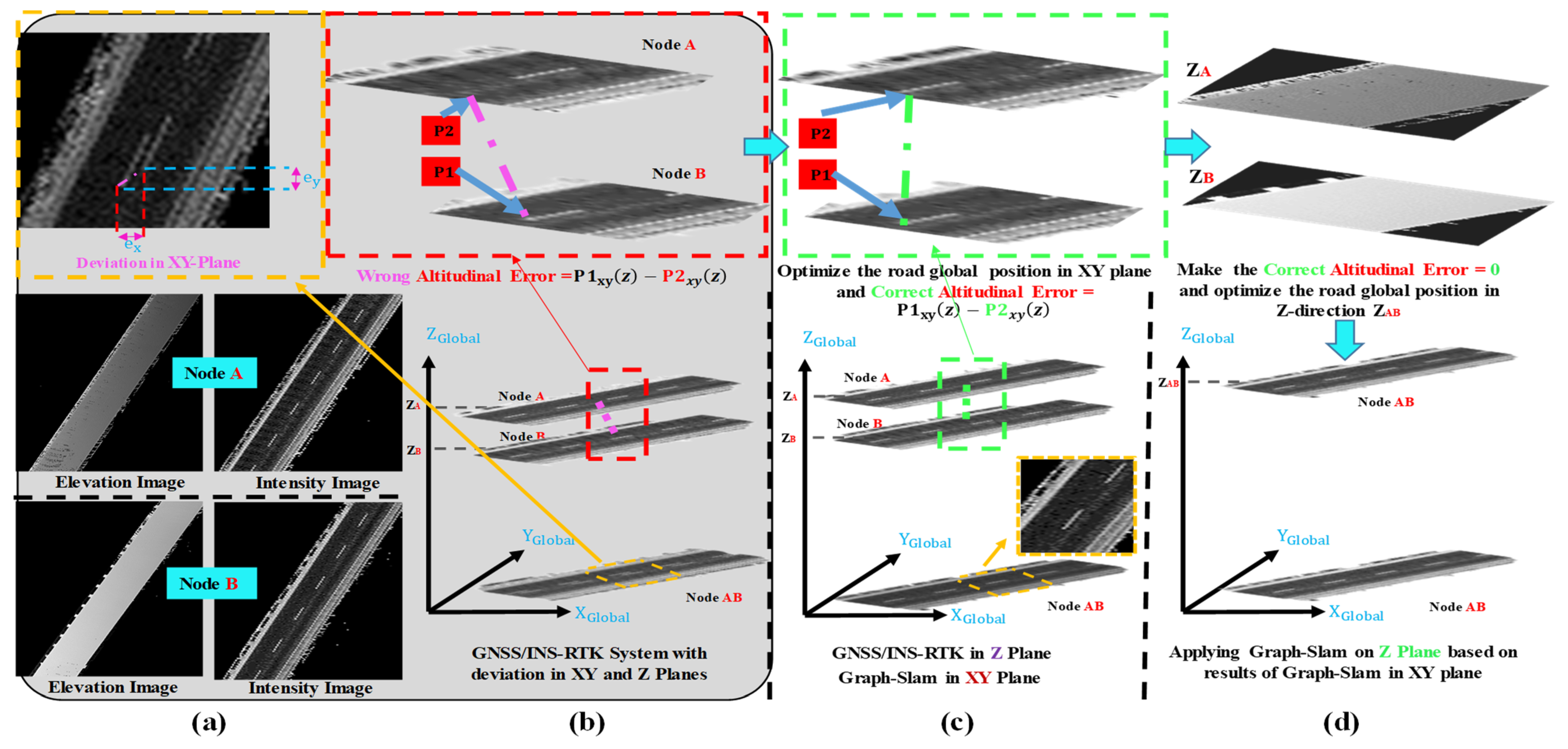
3. The Proposed Graph SLAM Framework (GS-XYZ)

3.1. Edge Selection and Calculation

The compensation of the relative-position errors is an essential step to apply GS. However, these errors represent local relationships between two nodes. The map generation in ACS can be achieved by optimizing the entire relative positions between nodes collectively and globally. Therefore, the coherency, consistency and accuracy between entire nodes in the map must be maintained and improved. This demand is achieved by properly designing the GS cost function. Figure 5a particularly demonstrates the relationships/edges between nodes in the XY plane. Each node possesses three types of edges: se-quential, anchoring and potential loop-closure. A sequential edge E^DR expresses the relationship between two consecutive nodes N_i and N_i−1 based on the top-left corners X and can be calculated using Equation (2).

$$E_{i,i-1}^{DR}=(f(X_{N_i}^{},X_{N_{i-1}}^{})-X_{N_{i,i-1}}^{DR}){\sum }_{i,i-1}^{-1}{(f(X_{N_i}^{},X_{N_{i-1}}^{})-X_{N_{i,i-1}}^{DR})}^T$$

(2)

where f(,) is a simple function to calculate the relative position, XDR is the edge constraint representing the dead reckoning relative position and Σ is the standard deviation of the vehicle velocity inside the driving area between N_i and N_i−1. These edges are necessary to preserve the smoothness of the road context and prevent deviations in a local area because of false loop-closure detection.

An anchoring edge E^GPS is used to place a node in the real world according to the GIR system as in Equation (3).

$$E_i^{GPS}=(X_{N_i}^{}-X_{N_i}^{GPS}){\Gamma }_i^{-1}{(X_{N_i}^{}-X_{N_i}^{GPS})}^T$$

(3)

where X^GPS is the edge constraint representing the node position based on the GIR system and Γ is the covariance error. These edges determine the position in ACS of merging many participating nodes in the same area based on the smallest covariance error.

An image edge E^img is mainly issued to compensate the XY relative position between two nodes in a revisited road segment and estimate the common area as in Equation (4).

$$E_{i,j}^{\mathrm{Im}g}=(f(X_{N_i}^{},X_{N_j}^{})-X_{N_{i,j}}^{\mathrm{Im}g}){\Omega }_{i,j}^{-1}{(f(X_{N_i}^{},X_{N_j}^{})-X_{N_{i,j}}^{\mathrm{Im}g})}^T$$

(4)

where X^img is the edge constraint based on matching the environmental features. The matching calculation is trigged when a loop-closure event between two nodes is detected. The identification strategy by top-left corners facilitates the detection process. The coordinates of the corners do not rely on the driving direction in the scanned environment. In other words, if the vehicle trajectory was in the upper lane (opposite driving direction) in Figure 3a, the xy-coordinates of the corner would be exactly the same. This makes the node distribution in ASC very coherent and homogenous. Therefore, the loop-closure events can be detected using a set of distance thresholds, such as the driving distance between two node candidates, the Euclidian distance between two top-left corners and the driving distance between two consecutive loop-closure events. Accordingly, a set of node-pairs that potentially share a considerable area in the real world is obtained.

As each node encodes a wide segment of the road surface in the intensity image, phase correlation (PhC) is applied on the detected loop-closure events to estimate X^img in Equation (4) and locally bring the common areas between every two nodes into the same xy-coordinates in ACS. PhC is widely utilized in the image processing and computer vision fields to solve various issues [24,25,26]. Technically, PhC relies on the shared pattern between two images to estimate xy-translation offsets using Fourier frequency transform (FFT) [27]. The robustness of PhC was the main motivation to invent the node strategy and design a new Graph SLAM framework. Moreover, PhC provides a correlation matrix that can be significantly employed to estimate the covariance error Ω in Equation (4). Accordingly, PhC has been modified to improve the performance on the intensity images, increase the matching accuracy and estimate the common area in each node of a loop-closure event. Figure 5b shows two nodes of a detected loop-closure event with the results of applying the enhanced PhC. The nodes are perfectly matched and provide the common area specifications in each node without any prior information of the top-left corner coordinates.

3.2. Cost Function Concept (Example: GS-XY)

The cost function is designed to optimize the edges and minimize the relative and global errors in the XY plane as in Equation (5).

$$X^{*}=\underset{z}{\arg \min }{\displaystyle \sum _{i,i-1}{E}_{i,i-1}^{DR}}+{\displaystyle \sum _{i,j}{E}_{i,j}^{\mathrm{Im}g}}+{\displaystyle \sum _i{E}_i^{GPS}}$$

(5)

The optimization process (GS-XY) can mathematically be expressed by Equation (6), which refers to the relationships of each node with other nodes in the map by H matrix.

$$\Delta X=-H^{-1}b$$

(6)

The diagonal elements in H imply the summing up of weighted confidences of the sequential and anchoring edges, whereas the off-diagonal elements indicate the loop-closure events weighted by PhC matching scores. The vector b demonstrates the weighted accumulative errors of the entire edges that are contacted to each node. A set of translation offsets ΔX is obtained by solving Equation (6) and added to the top-left corners of the map nodes. The offsets move the nodes in the XY plane to the optimal positions in ACS, eliminating the ghosting effects and maintaining smooth road contexts.

3.3. Transforming GS-XY to GS-Z

The style of applying GS-Z on the elevation images is similar to GS-XY in terms of edge concept and cost-function design. On the other hand, calculating the elevation relative position errors should be strategized. In our previous work [21], the detected common areas by PhC at each loop-closure event were used to calculate the elevation errors. PhC may provide inaccurate lateral matching results in the wide roads, where the shared landmarks are not sufficient (Figure 6a), as well as wrong correspondences in the longitudinal direction between nodes of critical environments, such as tunnels, where the road pattern is identical. This leads to wrong calculations of the altitudinal errors in the common areas, increases the excluded edges in the optimization process and may negatively influence the optimization process in the Z plane by producing unsmooth local road context in the elevation maps.

The inaccurate PhC matching results are overcome by adding ΔX of GS-XY to the nodes’ top-left corners as demonstrated in Figure 6b. Accordingly, a common area in node_i (U × V) can be projected accurately to node_j regardless of the previously estimated area by PhC in node_j. These two areas are guaranteed to represent the same environment in the real world, and they must be in the same Z-level. Therefore, a loop-closure elevation edge Z^img is precisely estimated by calculating the average altitudinal error in Equation (7) between the two areas based on the true pixel correspondences.

$$Z_{N_{i,j}}^{\mathrm{Im}g}=\frac{1}{UV}{\displaystyle \sum _{u=0}^U{\displaystyle \sum _{v=0}^V{z}_{N_i}(u,v)-}}{z}_{N_j}(u,v);z_{N_i}(u,v)\ne 0,z_{N_j}(u,v)\ne 0$$

(7)

The cost function of GS-Z is designed in Equation (8) using similar edge concepts of GS-XY as illustrated in Figure 6c, and a set of Z-offsets is obtained accordingly. A z-offset of an ith node is added to the entire pixels in the corresponding elevation image, i.e., updating the altitudinal average value for identifying the node in the Z plane. The elevation map is then generated accurately by rearranging the nodes’ elevation images in ACS.

$$Z^{*}=\underset{z}{\arg \min }{\displaystyle \sum _{i,i-1}{Z}_{i,i-1}^{DR}}+{\displaystyle \sum _{i,j}{Z}_{i,j}^{\mathrm{Im}g}}+{\displaystyle \sum _i{Z}_i^{GPS}}$$

(8)

4. Experimental Platform and Test Course

4.1. Platform Configuration and Framework Setups

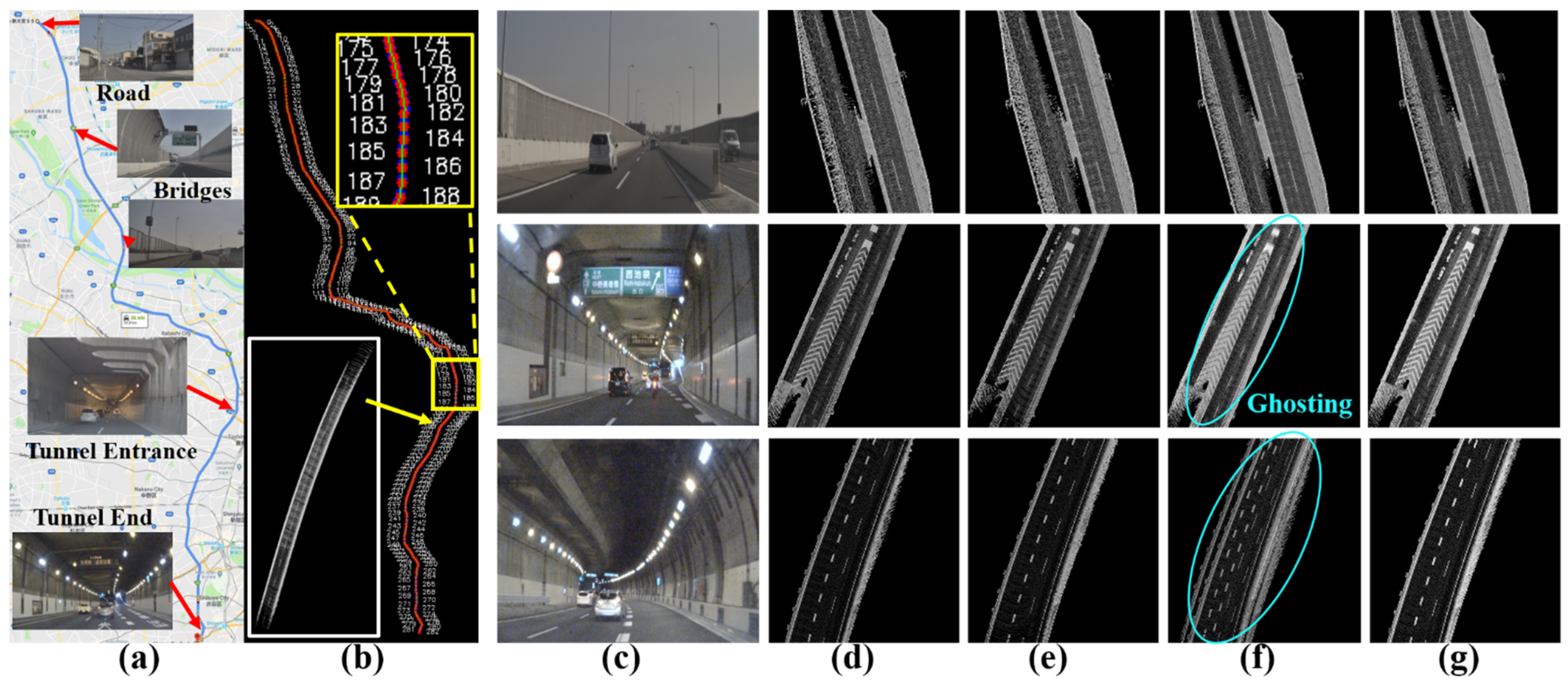
Figure 7 shows the robotics platform used to collect map data. The vehicle is equipped with Velodyne LIDAR 64 for 360 scanning the environment and generating 3D point clouds. A coupled GIR system POSLV 220 is deployed in the trunk to receive satellite signals and estimate the vehicle position, acceleration, velocity and angular parameters. After collecting the map data, these measurements are post-processed to produce very accurate vehicle trajectories. LIDAR point clouds are then assigned to the trajectories to generate the maps [28].

According to the proposed framework, the size of a LIDAR-frame w × h is 512 × 512. The area threshold of a node to be generated is set to W.H = 1 M pixels. The pixel resolution is 0.125 m in the intensity-image and 0.01 m in the elevation image (direct save of the altitudinal information in a floating matrix). A LIDAR frame is generated every 100 ms, whereas the GIR system provides measurements within 10 ms. Therefore, a synchronization process is technically applied based on the timestamps to estimate the vehicle position as soon as a LIDAR frame is created. Accordingly, DR is used to estimate the vehicle position in XY and Z planes as explained in the node strategy. The processing unit has Intel-Core™ i7-6700 CPU working at 3.40 GH with 64 GB of RAM. The operating system is Windows 10 64X and the localization system was coded using VS-2010 C++ environment with integrating OpenCV 2.3.1 and Eigen libraries. The FFTW library was integrated into the programing environments and the processing time to estimate that the relative position between two nodes by PhC is around 20 ms and [29].

4.2. Test Course

The proposed framework has been tested in a critical environment to emphasize the robustness and reliability against the GIR system. Tunnels are very efficient environments to test any proposed SLAM method because they have no surrounding environmental features that may differ according to the vehicle positions or the driving lane, i.e., the road surface is identical in the two trials, and deviations can easily be observed on the painted landmarks. Yamate Tunnel is an 18.2-km highway road in Tokyo and ends at Ohashii Junction with a 30-m underground depth. It is the world’s longest tunnel and consists of two tubes. Each tube enables a single driving direction and contains two lanes. In order to extend the course length and increase the size of the map data, we started to drive the vehicle from Yono Junction as shown in Figure 8a. Therefore, the course length becomes 34 km, including a considerable open-sky area before entering the tunnel. As driving inside a tube is in one direction, we scanned the first tube two times and drove at different velocities for each scan. This increases the node number and makes the optimization of relationships between nodes very challenging as detailed in the next section.

5. Results and Discussion

5.1. Graph SLAM in the XY Plane

The node strategy has led to a unique design of GS framework that reduces the map data size and decreases the processing time of the optimization process. This allows researchers to maintain a simple and easy arrangement of intensity and elevation values of the road-surface in the real world. The decomposition of the map into these two components facilitates the constitution of the relationships between nodes by the cost function. The test course was scanned by 283 nodes (16,041 point clouds) in the first scan and by 285 nodes (15,473 point clouds) in the second scan. The difference in the node numbers is intentionally created by a slight change of the starting point, and the difference in the point cloud number indicates different velocities of the vehicle during the two scans. Obviously, loop-closure events of the two scans are existent continuously along the course as illustrated in Figure 8b. Figure 8c–g show three loop-closure edges with the merged images based on PhC and GIR. The nodes of the two maps in open-sky areas are accurately combined in ACS using GIR in Figure 8f. On the other hand, the two scans are considerably deviated by GIR at the entrance of Yamate Tunnel until its end. The relative-position X^img is precisely estimated using PhC by extracting the coordinates of the common areas in the corresponding nodes’ images as shown in Figure 8g. In order to provide a holistic assessment of PhC against GIR results, Figure 9a illustrates the loop-closure edges along the two scans. Each edge represents the difference in x and y directions of the top-left coordinates of the detected common areas between a pair of nodes. The difference should be small because a common area represents the same road segment in the real world as can be observed in Figure 8. GIR is massively affected inside the tunnel and the two scans have large deviations up to 4 m. This indicates the low map quality and the risky ghosting effects in representing the road surface. Moreover, it refers to different locations of the road segments in ACS.

PhC has sufficiently compensated the relative position errors based on matching the static environmental features in the node images. The cost function significantly assigns these compensations to the graph with the sequential and anchoring edges. The graph is then optimized, and a set of translation offsets of the top-left corners is obtained. Figure 9b–c show the GS offsets of the nodes in Y and X directions. The offsets are small in the open-sky areas, i.e., the nodes have same positions of GIR in ACS. This proves the robustness of the proposed framework to generate the same map quality of GIR in such environments because GIR maps can be considered as ground-truth. The offset profiles demonstrate a continuous change of the nodes’ positions inside the tunnel. This implies the reliability of the proposed framework to detect the low accurate areas and fix the relative-position errors accordingly. In addition, the offsets differ between the two maps at the same area.

This implicitly illustrates the influences of the anchoring edges to determine the global position of the combined map based on the correct integration of the relevant covariance errors in ACS. Figure 10 shows images of GIR and GS-XY maps at different places inside Yamate Tunnel. The GIR map images demonstrate different ghosting patterns, whereas the GS map provides accurate road-surface representations. This indicates the robustness of the framework to constitute and optimize the node positions significantly regardless of the road structure and environment types.

5.2. Graph SLAM in the Z Plane

Figure 9a contains spiking peaks inside the open-sky area. The bridge and tunnel road segments are almost identical in the two scans because of the surrounding walls and barriers. Therefore, it is difficult for PhC to accurately recover the relative-position errors in the longitudinal direction. Figure 11a–d show the two scans’ nodes of the highest peak in Figure 9a (open-sky) with the combined results using PhC and the GIR system, respectively. PhC provides an inaccurate estimation of the longitudinal relative-position, whereas a true combination is obtained in the GIR combined map image. Figure 11e shows the corresponding GS map image with the same quality of GIR map. Thus, GS-XY can be considered as a filtration process of wrong results of PhC for applying GS-Z as observed by applying our previous work [21]. This increases the number of correct altitudinal edges between nodes. Moreover, decomposing GS-XYZ into two phases in the XY plane and then the Z plane makes the calculation of altitudinal edges very simple and easy. This is because the covariance estimation of Z^img can be set to a constant scalar for the entire altitudinal edges in the map.

Figure 12a shows the accuracy profiles of the GIR system in the Z-direction of the two scans. Obviously, the profiles demonstrate higher satellite signal quality in the open-sky area with different accuracies in some segments because of changing the traffic flow and driving scenarios along the two scans. The profiles considerably and gradually become inaccurate inside the Yamate Tunnel. Figure 12b in the red profile illustrates the altitudinal relative errors in the common areas between nodes of the two scans according to the GIR elevation map. The profile indicates huge altitudinal errors inside the tunnel because of representing same road segments in the real world. Figure 12b in the green profile shows the altitudinal error after applying GS-Z and distributing the obtained z-offsets on the nodes in the two scans. GS-Z has perfectly reduced the altitudinal error, significantly recovering the damaged and critical areas compared to the GIR elevation map.

As an edge represents a loop-closure between two nodes and in order to highlight the reliability of GS-XYZ to publish the elevation map in ACS, two particular edges/loop-closures are shown in Figure 13a,b. The first edge represents the maximum altitudinal error inside the Yamate Tunnel (1.2 m in Figure 12a), whereas the second edge is closer to the end of the tunnel. For more precise evaluation, the trajectory of the vehicle in node_j (reference) is projected onto node_j (target), accurately based on the resultant common areas by GS-XY as indicated by the dotted lines in Figure 13c,d. The altitudinal error is then calculated at each vehicle position by subtracting the corresponding values in the elevation images of GIR and GS-XYZ. It can be observed that the GIR profiles have considerable and different distances in Z-direction in both edges. This indicates the altitudinal relative position errors between the two scans as well as the global position errors of the elevation map in these two local road segments. The GS profiles are perfectly aligned to make the altitudinal relative errors as small as possible and bring the common areas in the loop-closure events into the same Z-level. One can observe that GS-XYZ has aligned the two scans at the middle distance in the first edge and closer to the first scan in the second edge. The two scans in the first edge (at 1.2 m error) has almost the same accuracy in the real world as indicated in Figure 12a (nodes 225 and 227), whereas the first scan possesses better accuracy at the end of the tunnel. This indicates the flexibility and robustness of the GS-Z cost function to publish the elevation map at the most accurate global positions in ACS. In order to prove that the global position of each road segment is determined with respect to the entire nodes in the map with preserving smooth road context in the Z-direction, Figure 13e shows the altitudinal errors of the GS-XYZ elevation map using the entire vehicle trajectory/positions of the first scan compared to the GIR elevation map. This figure indicates that the GS-XYZ map is very accurate and can be used to localize autonomous vehicles precisely as well as sufficiently enable other applications, such as object distance estimation and roll/pitch angle calibration. This indicates the robustness of the designed cost function to compensate the altitudinal error locally between every two nodes of a loop-closure event and globally with respect to the other events in the entire map in ACS.

6. Conclusions

We proposed a relatively simple Graph SLAM framework to generate accurate LIDAR intensity and elevation maps. The framework operates in the node level and image domain instead of the conventional strategies of operating in the vehicle position level and point cloud domain. This reduced the data size in the optimization process, allowing researchers to utilize phase correlation to efficiently compensate the xy relative position errors based on road surface representations, and facilitated constitution of the relationships between nodes regardless of the vehicle trajectory. Moreover, the optimization process is decomposed into two phases to apply Graph SLAM in the XY plane and accordingly optimize the elevation position in the Z plane. This unique tactic has been proved to significantly reduce the influences of changing the high environmental features by traffic flow or driving scenarios compared to the conventional strategies of applying SLAM in the XYZ plane at once and guarantee precise generation of the intensity maps in the XY plane. In addition, this tactic enabled accurate determination of the elevation errors and facilitated the edge calculation and covariance estimation of the relationships between nodes in the Z plane. The experimental results have verified the robustness and reliability of the proposed framework to generate very accurate and coherent 2.5D maps in the world’s longest tunnel at 30 m depth underground compared to an accurate and expensive GNSS/INS-RTK system. Therefore, the proposed framework increases the scalability of the mapping module to represent the real world precisely and enable safe autonomous driving.

7. Patents

This work was patented in Japan in 2020 with the global number: 2020-090099.

References

1. Aldibaja, M.; Suganuma, N.; Yoneda, K. Robust intensity based localization method for autonomous driving on snow-wet road surface. In Proceedings of the IEEE Transactions on Industrial Informatics; 2017; Volume 13, pp. 2369–2378. Available online: https://ieeexplore.ieee.org/abstract/document/7944675 (accessed on 3 October 2021).
2. Pendleton, S.D.; Andersen, H.; Du, X.; Shen, X.; Meghjani, M.; Eng, Y.H.; Rus, D.; Ang, M.H. Perception, planning, control, and coordination for autonomous vehicles. Machines 2017, 5, 6. [Google Scholar] [CrossRef]
3. Kuramoto, A.; Aldibaja, M.; Yanase, R.; Kameyama, J.; Yoneda, K.; Suganuma, N. Mono-Camera based 3D object tracking strategy for autonomous vehicles. In Proceedings of the 2018 IEEE Intelligent Vehicles Symposium (IV), Changshu, China, 26–30 June 2018; pp. 459–464. [Google Scholar]
4. Thrun, S.; Montemerlo, M. The graph SLAM algorithm with applications to large-scale mapping of urban structures. Int. J. Robot. Res. 2006, 25, 403. [Google Scholar] [CrossRef]
5. Grisetti, G.; Kümmerle, R.; Stachniss, C.; Burgard, W. A Tutorial on Graph-Based SLAM. Proc. IEEE Intell. Transp. Syst. Mag. 2010, 2, 31–43. Available online: https://ieeexplore.ieee.org/document/5681215 (accessed on 3 October 2021). [CrossRef]
6. Olson, E.; Agarwal, P. Inference on networks of mixtures for robust robot mapping. Int. J. Robot. Res. 2013, 32, 826–840. [Google Scholar] [CrossRef]
7. Roh, H.; Jeong, J.; Cho, Y.; Kim, A. Accurate mobile urban mapping via digital map-based SLAM. Sensors 2016, 16, 1315. [Google Scholar] [CrossRef] [PubMed] [Green Version]
8. Triebel, R.; Pfaff, P.; Burgard, W. Multi-level surface maps for outdoor terrain mapping and loop closing. In Proceedings of the IEEE/RSJ International Conference Intelligent Robots and Systems (IROS), Beijing, China, 9–15 October 2006; pp. 2276–2282. [Google Scholar]
9. He, Y.; Liang, B.; Yang, J.; Li, S.; He, J. An iterative closest points algorithm for registration of 3D laser scanner point clouds with Geometric Features. Sensors 2017, 17, 1862. [Google Scholar] [CrossRef] [PubMed] [Green Version]
10. Shan, T.; Englot, B. LeGO-LOAM: Lightweight and ground-optimized Lidar odometry and mapping on variable terrain. In Proceedings of the IEEE/RSJ International Conference on Intelligent Robots and Systems (IROS), Madrid, Spain, 1–5 October 2018; pp. 4758–4765. [Google Scholar] [CrossRef]
11. Shan, T.; Englot, B.; Meyers, D.; Wang, W.; Ratti, C.; Rus, D. Lio-sam: Tightly-coupled lidar inertial odometry via smoothing and mapping. In Proceedings of the 2020 IEEE/RSJ International Conference on Intelligent Robots and Systems (IROS), Las Vegas, NV, USA, 24 October 2020–24 January 2021; pp. 5135–5142. [Google Scholar] [CrossRef]
12. Cadena, C.; Carlone, L.; Carrillo, H.; Latif, Y.; Scaramuzza, D.; Neira, J.; Reid, I.D.; Leonard, J.J. Simultaneous localization and mapping: Present, future, and the robust-perception Age. Proc. IEEE Trans. Robot. 2016, 32, 1309–1332. Available online: https://ieeexplore.ieee.org/document/7747236 (accessed on 3 October 2021). [CrossRef] [Green Version]
13. Wolcott, R.; Eustice, R. Fast lidar localization using multiresolution gaussian mixture maps. In Proceedings of the IEEE International Conference on Robotics and Automation (ICRA), Seattle, WA, USA, 26–30 May 2015; pp. 2814–2821. [Google Scholar]
14. Khot, L.R.; Tang, L.; Steward, B.L.; Han, S. Sensor fusion for roll and pitch estimation improvement of an agricultural sprayer Vehicle. In Proceedings of the American Society of Agricultural and Biological Engineers; 2008; Volume 101, pp. 13–20. Available online: https://dr.lib.iastate.edu/entities/publication/b11aae8f-ccf5-4de8-9a65-d0ec7701be22 (accessed on 3 October 2021).
15. Li, X.; Gao, Z.; Chen, X.; Sun, S.; Liu, J. Research on Estimation Method of Geometric Features of Structured Negative Obstacle Based on Single-Frame 3D Laser Point Cloud. Information 2021, 12, 235. [Google Scholar] [CrossRef]
16. Lewis, J.P. Fast normalized cross-correlation. Vis. Interface 1993, 10, 120–123. [Google Scholar]
17. Besl, P.J.; McKay, H.D. A method for registration of 3-D shapes. Proc. IEEE Trans. Pattern Anal. Mach. Intell. 1992, 14, 239–256. Available online: https://ieeexplore.ieee.org/document/121791 (accessed on 3 October 2021). [CrossRef]
18. Biber, P.; Straßer, W. The normal distributions transform: A new approach to laser scan matching. In Proceedings of the International Conference on Intelligent Robots and Systems, Las Vegas, NV, USA, 27–31 October 2003; pp. 2743–2748. [Google Scholar]
19. Sakai, T.; Koide, K.; Miura, J.; Oishi, S. Large-scale 3D outdoor mapping and on-line localization using 3D-2D matching. In Proceedings of the IEEE/SICE International Symposium on System Integration (SII), Taipei, Taiwan, 11–14 December 2017; pp. 829–834. [Google Scholar]
20. Nam, T.H.; Shim, J.H.; Cho, Y.I. A 2.5D Map-Based mobile robot localization via cooperation of aerial and ground robots. Sensors 2017, 17, 2730. [Google Scholar] [CrossRef] [PubMed] [Green Version]
21. Aldibaja, M.; Yanase, R.; Kim, T.; Kuramoto, A.; Yoneda, K.; Suganuma, N. Accurate Elevation Maps based Graph-Slam Framework for Autonomous Driving. In Proceedings of the IEEE Intelligent Vehicles Symposium (IV), Paris, France, 9–12 June 2019; pp. 1254–1261. [Google Scholar] [CrossRef]
22. Sun, L.; Zhao, J.; He, X.; Ye, C. DLO: Direct LiDAR Odometry for 2.5D Outdoor Environment. In Proceedings of the 2018 IEEE Intelligent Vehicles Symposium (IV), Changshu, China, 26–30 June 2018; pp. 1–5. [Google Scholar]
23. Yoon, J.; Kim, B. Vehicle Position Estimation Using Tire Model in Information Science and Applications; Springer: Berlin, Germany, 2015; Volume 339, pp. 761–768. [Google Scholar]
24. Ahuja, K.; Tuli, K. Object recognition by template matching using correlations and phase angle method. Int. J. Adv. Res. Comput. Commun. Eng. 2013, 2, 1368–1372. Available online: https://www.ijarcce.com/upload/2013/march/11-kavita%20ahuja%20-%20object%20recognition-c.pdf (accessed on 3 October 2021).
25. Sarvaiya, J.; Patnaik, S.; Kothari, K. Image registration using log polar transform and phase correlation to recover higher scale. J. Pattern Recognit. Res. 2012, 7, 90–105. [Google Scholar] [CrossRef]
26. Liang, Y. Phase-Correlation Motion Estimation. EE392J Project Report. 2000. Available online: https://web.stanford.edu/class/ee392j/Winter2002/student_projects_final_Winter2000.html (accessed on 3 October 2021).
27. Almonacid-Caballer, J.; Pardo-Pascual, J.E.; Ruiz, L.A. Evaluating Fourier cross-correlation sub-pixel registration in landsat images. Remote Sens. 2017, 9, 1051. [Google Scholar] [CrossRef] [Green Version]
28. Aldibaja, M.; Suganuma, N.; Yoneda, K. LIDAR-Data accumulation strategy to generate high definition maps for autonomous vehicles. In Proceedings of the IEEE Conference on Multisensor Fusion and Integration for Intelligent Systems, Daegu, Korea, 16–18 November 2017; pp. 422–428. [Google Scholar] [CrossRef]
29. Frigo, M.; Johnson, S.G. The Design and Implementation of FFTW3. Proc. IEEE 2005, 93, 216–231. Available online: https://ieeexplore.ieee.org/document/1386650 (accessed on 3 October 2021).
Figure 1. (a) Ghosting effects (duplication of road landmarks because of scanning the segment twice with different positioning accuracies by GNSS/INS-RTK) in the map and multiple matching patterns with the observation point cloud. (b) Identical map without ghosting and the corresponding matching result.
Remotesensing 13 05066 g001
Figure 2. (a) Featureless wide road in the Z-direction. (b) Preventing static features to be encoded at a traffic signal by stopped cars.
Remotesensing 13 05066 g002
Figure 3. Accurate node strategy. (a) Intensity image to represent road surface at 0.3 m in the Z-direction with surrounding environments and top-left corner identification tactic. (b) Elevation image.
Remotesensing 13 05066 g003
Figure 4. Graph SLAM in node level. (a) Two nodes at a loop-closure event with intensity and elevation images. (b) Deviations (relative position errors) between nodes in the XY and Z planes by the GIR system. (c) Applying GS-XY on intensity images by eliminating ghostings and aligning the road perfectly. (d) Applying GS-Z on elevation images using correct calculations of altitudinal errors by GS-XY and making altitudinal errors as small as possible.
Remotesensing 13 05066 g004
Figure 5. (a) Relationship between nodes in the XY plane and edge types of GS-XY cost function. (b) Applying PhC to merge two nodes (N3 and Nt) based on matching road landmarks with estimating common areas for loop-closure edges.
Remotesensing 13 05066 g005
Figure 6. (a) Two nodes merged wrongly by PhC. (b) Correct merging by GS-XY showing the correct position of the common area in each node. (c) GS-framework in the Z plane applied on elevation images based on projected areas by GS-XY.
Remotesensing 13 05066 g006
Figure 7. Experimental platform with sensor configurations.
Remotesensing 13 05066 g007
Figure 8. Yamate Tunnel in Tokyo. (a) Two-times scanned course starting at Yono Junction and ending with the Yamate Tunnel. (b) Top-left corners of course nodes showing loop-closure lines (green) and the first node in the tunnel. (cg) Three loop-closure events along the course demonstrating in rows: open-sky area, Yamate Tunnel entrance and end of the tunnel. (c) Camera image. (d) Patch of a node image in first scan. (e) Same area in second scan. (f) Merging scans based on GNSS/INS-RTK. (g) Merging scans based on phase correlation.
Remotesensing 13 05066 g008
Figure 9. (a) Loop-closure edges (coordinate difference) of the common areas between two scans in x and y directions obtained by GNSS/INS-RTK system and phase correlation on the node images. (b) The proposed GS-XY’s Y-offsets to top-left corners of nodes in the first and second scans. (c) X-offsets to two scans.
Remotesensing 13 05066 g009
Figure 10. Wrong combined node images inside the Yamate Tunnel by GIR (first row) and accurate combination by GS-XY framework (bottom).
Remotesensing 13 05066 g010
Figure 11. Robustness of GS-XY against wrong loop-closure edges. (a) First scan. (b) Second scan. (c) Wrong matching of the two images using phase correlation. (d) Accurate combination of two maps by the GNSS/INS-RTK system. (e) Accurate combination of the two images using GS-XY to recover the wrong result in (c) based on optimizing the entire relationships between scans’ nodes by the designed cost function. It can be observed that the map images in (d,c) are denser than those in (a,b) to indicate the importance to safely combine and update maps in such highway environments.
Remotesensing 13 05066 g011
Figure 12. (a) Standard deviation of the GIR system in the Z plane showing unstable accuracy along elevation images inside the Yamate Tunnel. (b) Large altitudinal differences between common areas in GIR elevation images (red profile) and the significant small differences after applying GS-Z (green profile). The dotted lines refer to edges in Figure 13.
Remotesensing 13 05066 g012
Figure 13. (a) Two nodes of the loop-closure edge with ID 340 in Figure 12a. (b) Two nodes of the loop-closure edge with ID 433 in Figure 12a. The common area in the reference node (first scan) is projected onto the target node (second scan) based on GS-XY. The vehicle trajectory in the first scan in the common area is then used to calculate the altitudinal error in the elevation images. (c,d) GS-Z and GIR elevation trajectories in the two scans in the common areas. A large elevation error was produced by GIR between the two scans, whereas GS-Z minimized the error and brought the node into same Z-level because of representing the same road segment in the real world. (e) The map elevation error between the two scans along the entire map (the first scan’s trajectory was used as reference).
Remotesensing 13 05066 g013
Publisher’s Note: MDPI stays neutral with regard to jurisdictional claims in published maps and institutional affiliations.