Semi-Supervised SAR Target Detection Based on an Improved Faster R-CNN

Abstract

In the remote sensing image processing field, the synthetic aperture radar (SAR) target-detection methods based on convolutional neural networks (CNNs) have gained remarkable performance relying on large-scale labeled data. However, it is hard to obtain many labeled SAR images. Semi-supervised learning is an effective way to address the issue of limited labels on SAR images because it uses unlabeled data. In this paper, we propose an improved faster regions with CNN features (R-CNN) method, with a decoding module and a domain-adaptation module called FDDA, for semi-supervised SAR target detection. In FDDA, the decoding module is adopted to reconstruct all the labeled and unlabeled samples. In this way, a large number of unlabeled SAR images can be utilized to help structure the latent space and learn the representative features of the SAR images, devoting attention to performance promotion. Moreover, the domain-adaptation module is further introduced to utilize the unlabeled SAR images to promote the discriminability of features with the assistance of the abundantly labeled optical remote sensing (ORS) images. Specifically, the transferable features between the ORS images and SAR images are learned to reduce the domain discrepancy via the mean embedding matching, and the knowledge of ORS images is transferred to the SAR images for target detection. Ultimately, the joint optimization of the detection loss, reconstruction, and domain adaptation constraints leads to the promising performance of the FDDA. The experimental results on the measured SAR image datasets and the ORS images dataset indicate that our method achieves superior SAR target detection performance with limited labeled SAR images.

1. Introduction

Synthetic aperture radar (SAR) is a moving radar system that works in all-day and all-weather conditions and is capable of producing high-quality remote sensing images. With the development of SAR imaging technology, SAR automatic target recognition (ATR) [1,2,3,4,5,6,7,8,9] has developed rapidly. In general, the SAR ATR system consists of the following stages: target detection [1,2,3,8,9], target discrimination [4,5], and target recognition [6,7]. As the first stage of SAR ATR, target detection is a significant research hotspot in remote sensing image processing.

Target detection focuses on deciding if a target of interest is present at a given position in an image. At present, much reasearch has been devoted to the field of SAR target detection, and the constant false alarm rate (CFAR) algorithm [8] is the most widely applied SAR target detection method. According to the statistical characteristics of clutter, the CFAR algorithm first calculates the detection threshold, which is then compared with the current pixel to determine whether the pixel is the target or clutter. In [9], a Gaussian-CFAR algorithm is developed based on the prior assumption that the background clutter in SAR images follows the Gaussian distribution, and the algorithm achieves excellent detection performance in some simple scenes. Though Gaussian CFAR does not need training samples, the performance of it will degrade in some complex scenes.

Deep-learning methods, especially convolutional neural networks (CNNs), have gained superior performance by the way of data-driven research in the target detection field. In recent years, the faster regions with convolutional neural network (R-CNN) features method has gained promising detection performance on SAR images. In [1], a novel model based on faster R-CNN is proposed by using the squeeze and excitation mechanisms, thus achieving better detection performance and faster speeds than the state-of-the-art method. In addition, Li et al. [3] develop an improved faster R-CNN model by introducing a feature-fusion module, a transfer learning idea, and a hard negative mining mechanism for ship detection. Moreover, Cui et al. [10] develop dense attention pyramid networks (DAPN) by using the feature extractor of faster R-CNN to fuse features of multiple layers and adaptively select significant scale features with an attention module, which performs well on multi-scale ship detection.

Although the above faster R-CNN-based methods have shown positive effects on the SAR target detection task, they require large-scale labeled training samples for model learning. In real situations, the labeling work for SAR images needs many labor and material resources. When lacking labels, the SAR target detection performance will degenerate greatly. In recent years, two main approaches, i.e., traditional semi-supervised approaches and domain-adaptation approaches, have been proposed to address the performance degeneration issue caused by limited labeled data in various fields [11,12,13,14,15,16,17,18,19,20,21,22].

The traditional semi-supervised methods focus on utilizing the unlabeled data to make up for the lack of label information. In the target detection field, many semi-supervised methods have already been developed to deal with the issue of limited labels. Rosenberg et al. [11] apply the self-training method to a traditional target detector for semi-supervised target detection. In [12], Zhang et al. apply the self-learning method to a target detection network, in which pseudo-labels of unlabeled slices are predicted by the trained classifier and the predicted negative slices are then applied for network training, which shows good detection results on optical images. Moreover, in [13], Sohn et al. develop a framework for an effective semi-supervised method based on self-training- and augmentation-driven consistency regularization (STAC), which has gained promising results in optical image detection. However, for SAR images with complex scenes, these self-learning methods [11,12,13] are at risk of selecting the wrong clutter as the targets of interest when producing pseudo-labels, which may lead to false detection. In [14], Wei et al. propose a novel semi-supervised method by utilizing lots of image-level labeled images to make up for the limit of target-level labeled images for SAR target detection. Though the method in [14] shows good performance, it needs image-level labels for all images, which also requires a certain labor resource. In addition, in image classification fields, the deep convolution auto-encoder [15] is a commonly used semi-supervised network that reconstructs all the labeled and unlabeled data. Some work [16], based on the auto-encoder network, can utilize the unlabeled data to extract more representative features for performance improvement, which illustrates that reconstruction performs well in semi-supervised learning.

In addition, the domain-adaptation (DA) [17] methods are another way of addressing the performance degeneration issue. They make the unlabeled data from the target domain participate in the learning process, which can promote the model performance on the target domain with the assistance of the data from the source domain that contains abundant labels. Adrian et al. [18] design a pixel-adaptation method to transfer the source images to the target domain by means of adaptive instance normalization; thus, the transferred images have labels. In addition, in [19], Chen et al. propose a hierarchical transferability calibration network (HTCN), which utilizes the features’ alignment to mitigate the distributional shifts for harmonizing the transferability and discriminability of the feature representations. Chen et al. [20] construct a adaptive-domain faster R-CNN (DAF) that enforces the feature distribution of the data in two related domains to be close via the domain classifier. These methods [18,19,20] have shown that the DA idea can take advantage of the unlabeled data to help model learning by introducing a related domain with abundant labels. Moreover, Guo et al. [21] propose the domain adaptation from the optical remote sensing (ORS) images to the SAR images to address the issue of the small labeled training data size in the SAR images, which validates the DA as an effective way of promoting the SAR detection performance by using the ORS images.

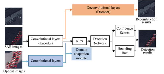
Inspired by the effectiveness of the auto-encoder and domain adaptation for semi-supervised learning, in this paper, we present an improved faster R-CNN with a decoding module and a domain-adaptation module (FDDA) for semi-supervised SAR target detection. In detail, we first incorporate a decoding module into the baseline faster R-CNN to build a semi-supervised detection framework, which contains a deep convolution auto-encoder branch that performs to recover the original input data from the latent feature. Thus, the unlabeled SAR images can participate in the training process, and more information about the SAR images can be explored by the decoding module, which is helpful to extract the features with strong representative capacity, and further, leads to better detection performance. The auto-encoder [22] is an unsupervised way of effectively exploring the representative features based on the data, but it is independent of the detection task. Furthermore, we aim to utilize the unlabeled SAR images to improve the discriminability of features for detection. Therefore, a domain-adaptation module is introduced by utilizing the ORS images with abundant labels to guide the learning of the features of SAR images. More specifically, our method adopts the maximum mean discrepancy (MMD) to learn the transferable features between the two domains, and then the discriminability of features of SAR images is improved with the label supervision of ORS images, which is beneficial to SAR target detection. Finally, the detection loss, reconstruction, and domain adaptation constraints are jointly optimized to train the FDDA, devoting attention to its promising SAR target detection performance with limited labeled SAR images.

With the proposed method, the SAR target detection task can be achieved with much less label cost, which greatly solves the problem of limited labeled SAR images. The principal contributions of this paper are listed as follows: (1) In the SAR target detection field, a semi-supervised detection network is constructed based on the auto-encoder framework. By reconstructing large-scale unlabeled SAR images, more information about the targets can be used to learn the representative features, which is beneficial to target detection. (2) The domain-adaptation idea is applied to realize the semi-supervised learning by introducing the ORS images with abundant labels. With the domain adaptation, the unlabeled SAR images participate in the training process to learn the discriminative features of SAR images, which further promotes the detection performance in the case of limited labels.

The remainder of this paper is organized as follows. In Section 3, some preliminaries covering faster R-CNN and MMD are provided. Section 3 presents the introduction to the proposed target detection method. In Section 4, we then show some experimental results and analyses of the SAR image datasets. Finally, the conclusion of this paper is shown in Section 5.

2. Preliminaries

This section introduces some related preliminaries, covering faster R-CNN and maximum mean discrepancy (MMD), which are helpful to understand the proposed model.

2.1. Faster R-CNN

As a two-stage detector, faster R-CNN is composed of the following three parts: (1) the base network; (2) the region-proposal network (RPN); (3) the region-of-interest (ROI) head. The base network projects the input image onto the latent space to obtain a feature map, which is then fed to the RPN. By the means of a low-dimensional convolution layer, the RPN is implemented by scanning each point on the learned feature map, and then multiple proposals are predicted for each point on the feature map. The proposals are operated with ROI pooling to obtain the feature vectors with the same size. After that, two nonlinear layers of full connection (FC) are adopted to predict the location and class of the obtained proposals [23]. Figure 1 presents the overall architecture of traditional faster R-CNN.

The total loss of faster R-CNN consists of the loss of the RPN branch and the loss of the ROI branch, which is expressed as:

$$L_{supervised}=L_{rpn}+L_{roi}$$

(1)

Moreover, the loss function of PRN $L_{rpn}$ is defined as:

$$L_{rpn}=\frac{1}{N_{cls}}{\displaystyle \sum _i{L}_{cls}\left(p_i,p_i^{*}\right)}+\lambda \frac{1}{N_{reg}}{\displaystyle \sum _i{p}_i^{*}{L}_{reg}\left(t_i,t_i^{*}\right)}$$

(2)

where $N_{cls}$ denotes the number of anchors in a minibatch, $N_{reg}$ represents the number of anchor locations, $L_{cls}$ and $L_{reg}$ denote the classification loss and regression loss, respectively, and $\lambda$ is the weight that makes the two loss terms roughly equally balanced, in practice, $\lambda =10$. Moreover, the log loss of two classes (target and background) can be further written as:

$$L_{cls}\left(p_i,p_i^{*}\right)=-\log \left[p_i^{*}{p}_i+(1-p_i^{*})(1-p_i)\right]$$

(3)

where $p_i^{*}$ and $p_i$ represent the ground-truth and the predicted probability of the $i\mathrm{th}$ anchor. The regression loss can be written as:

$$L_{reg}\left(t_i,t_i^{*}\right)=R\left(t_i-t_i^{*}\right)$$

(4)

where $t_i=\left\{t_x,t_y,t_w,t_h\right\}$ is a vector indicating the predicted shift, and $t_i^{*}$ represents the true box coordinate. $R$ denotes the smooth L1 loss, and is defined as:

$$smoot{h}_{L_1}\left(x\right)=\{\begin{array}{l}0.5x^2\hspace{1em}\hspace{1em}\hspace{1em} if\left|x\right|<1\\ \left|x\right|-0.5\hspace{1em}\hspace{1em}otherwise\end{array}$$

(5)

In addition, the loss of the ROI head is expressed as:

$$L_{roi}=\frac{1}{N_{cls}^{roi}}{\displaystyle \sum _i{L}_{cls}\left(p,u\right)}+\lambda \frac{1}{N_{reg}^{roi}}{\displaystyle \sum _{i}u{L}_{reg}\left(t^u,v\right)}$$

(6)

where $N_{cls}^{roi}$ and $N_{cls}^{roi}$ denote the number of predicted targets and locations in a minibatch; $p$ and $u$ represent the predicted probability and the ground-truth of class, and $L_{cls}\left(p,u\right)$ denotes the cross entropy loss of multiple classes if the number of classes is larger than 2; $t^u$ and $v$ denote the predicted locations of and the ground-truth of the bounding boxes. Although the original paper [23] adopts the four-step method of alternating training to train faster R-CNN, most recent achievements directly utilize the end-to-end methods of approximate joint training, which converge much faster.

2.2. Maximum Mean Discrepancy (MMD)

The basic statistical test criterion of maximum mean discrepancy (MMD) is as follows: based on the samples generated by two distributions, $p$ and $q$, MMD first obtains the means of the samples mapped by a function $f$ from the two distributions, and then the mean discrepancy between the mapped samples from the two distributions can be obtained. As an effective non-parametric criterion, the MMD can be used to measure the distribution discrepancy for the samples from two different datasets.

Recently, the MMD constraint has been applied in domain adaptation. Usually, the domain adaptation aims to transfer the abundant knowledge of the source domain to the target domain. However, there is great discrepancy between different domains. The MMD can be utilized to measure the distribution discrepancy between the target domain and the source domain. Here, let ${\mathcal{D}}_t={\left\{x_i^t\right\}}_{i=1}^{N_t}$ denote the dataset from the target domain with $N_t$ SAR images, and ${\mathcal{D}}_s={\left\{x_i^s\right\}}_{i=1}^{N_s}$ represent the dataset from the source domain with $N_s$ ORS images. $x_i^t$ and $x_i^s$ are matrices, and they are the real (magnitude) pixels of the images. ${\mathcal{D}}_t={\left\{x_i^t\right\}}_{i=1}^{N_t}$ and ${\mathcal{D}}_s={\left\{x_i^s\right\}}_{i=1}^{N_s}$ are two datasets drawn from IID distributions $p$ and $q$, respectively. For the data from the two domains, we cannot specify the distributions $p$ and $q$ for the datasets ${\mathcal{D}}_t$ and ${\mathcal{D}}_s$, but we can know that the data in ${\mathcal{D}}_t$ have different statistical characteristics from the data in ${\mathcal{D}}_s$. The MMD criterion can be utilized to measure the distribution discrepancy for the data from the two different distributions without knowing the specific form for distributions $p$ and $q$. In MMD, if there exists a mapping function $f$, the mapping of the data from the target domain is similar to that of the source domain. In detail, the distribution discrepancy of the data with different distributions can be calculated with MMD as:

$$L_{MMD}={\Vert \frac{1}{N_s}{\displaystyle \sum _{i=1}^{N_s}f\left(x_i^s\right)}-\frac{1}{N_t}{\displaystyle \sum _{i=1}^{N_t}f\left(x_i^t\right)}\Vert }_2^2$$

(7)

where ${\Vert \cdot \Vert }_2$ denotes the L2-norm; $x_i^s$ and $x_i^t$ represent the samples from the two distributions $p$ and $q$, respectively. In general, the mapping function $f$ in MMD, being a kernel function, has a specific expression, and it is often chosen as the Gaussian kernel function, since the Gaussian kernel can map the data into infinite-dimensional space, which is more expressive. Thus, Equation (7) can be further expanded as:

$$L_{MMD}=\frac{1}{{\left(N_s\right)}^2}{\displaystyle \sum _{i=1}^{N_s}k\left(x_i^s,x_i^s\right)}-\frac{1}{N_s{N}_t}{\displaystyle \sum _{i=1}^{N_s}k\left(x_i^s,x_i^t\right)}+\frac{1}{{\left(N_t\right)}^2}{\displaystyle \sum _{i=1}^{N_t}k\left(x_i^t,x_i^t\right)}$$

(8)

where $k\left(\cdot ,\cdot \right)$ is set as the Gaussian kernel function $k\left(x_i^s,x_i^t\right)=e^{-{\Vert x_i^s-x_i^t\Vert }^2/\gamma }$, with $\gamma$ being the kernel parameter.

In this paper, the MMD is utilized to measure the distribution discrepancy between the features of SAR and the optical remote sensing data. The MMD can be written as:

$$L_{MMD}=\frac{1}{{\left(N_s\right)}^2}{\displaystyle \sum _{i=1}^{N_s}k\left(z_i^s,z_i^s\right)}-\frac{1}{N_s{N}_t}{\displaystyle \sum _{i=1}^{N_s}k\left(z_i^s,z_i^t\right)}+\frac{1}{{\left(N_t\right)}^2}{\displaystyle \sum _{i=1}^{N_t}k\left(z_i^t,z_i^t\right)}$$

(9)

where $z_i^t,z_i^s$ denotes the features of the $i\mathrm{th}$ SAR and optical remote sensing images that are obtained via the feature-extraction networks. By minimizing the $L_{MMD}$, our network is optimized to extract the features $z_i^t,z_i^s$ that have the minimum distribution discrepancy after being mapped to the RKHS via the Gaussian kernel function. Therefore, in our method, MMD performs to help learn the transferable features between the SAR and optical remote sensing data. A more detailed description of how the MMD is utilized in our proposed method can be found in Section 3.1.2.

3. The Proposed Method

When lacking large-scale labeled training data, the existing SAR target detection methods will be faced with the severe problem of performance degradation. To address the issue, this paper constructs a semi-supervised method based on faster R-CNN. We first introduce a decoding module into faster R-CNN to build a convolution auto-encoder structure that can excavate more information from many unlabeled SAR images, and then learn the representative features for target detection. In addition, we notice that the ORS images can be labeled more easily; thus, the abundantly labeled ORS images can be collected to learn the discriminative features for target detection. In our method, we utilize a domain-adaptation module to transfer the abundant information of the labeled ORS images to the SAR images. Thus, the ORS images are taken as the supervisior of the feature-extraction of the SAR images, which improves the SAR target detection performance with limited training labels. We, ultimately, build the improved faster R-CNN with a decoding module and a domain-adaptation module (FDDA). In this section, a detailed introduction to the FDDA will be presented.

3.1. Model Structure

Let ${\mathcal{D}}_s={\{(x_i^s,y_i^s)\}}_{i=1}^{N_s}$ represent the source domain dataset (ORS image dataset) with $N_s$ denoting the number of ORS images, and $x_i^s$ represent the $i\mathrm{th}$ ($i\in \left\{1,\cdots ,N_s\right\}$) optical remote sensing image that is a matrix and that is the real (magnitude) pixels of the images. The label $y_i^s$ denotes the location and class label of targets in the $i\mathrm{th}$ image $x_i^s$ and is a set of vectors. More specifically, assuming that there are $K$ targets in the image $x_i^s$, the label $y_i^s$ represents ${\left\{t_x^k,t_y^k,t_w^k,t_h^k,l^k\right\}}_{k=1}^K$, where $t_x^k,t_y^k$ denotes the center coordinate of the bounding box for the $k\mathrm{th}$ target, $t_w^k,t_h^k$ denotes its length and width, $l^k$ denotes the class number of the $k\mathrm{th}$ target, and $t_x^k,t_y^k,t_w^k,t_h^k,l^k$ are real scalar numbers. Let ${\mathcal{D}}_t={\left\{x_i^t\right\}}_{i=1}^{N_t}$ denote the target domain dataset (SAR image dataset) with $N_t$ denoting the number of SAR images, and $x_i^t$ represent the $i\mathrm{th}$ ($i\in \left\{1,\cdots ,N_t\right\}$) SAR image that is a matrix, and that is also the real (magnitude) pixels of the images. The target domain dataset $D_t=D_l\cup D_u$ contains the labeled data ${\mathcal{D}}_l={\{(x_i^l,y_i^l)\}}_{i=1}^{N_l}$ with $N_l$ samples, and the unlabeled data ${\mathcal{D}}_u={\left\{x_i^u\right\}}_{i=1}^{N_u}$ with $N_u$ samples. In the semi-supervised adaptation, the target domain has only a small number of labeled examples, i.e., $N_l\ll N_u$.

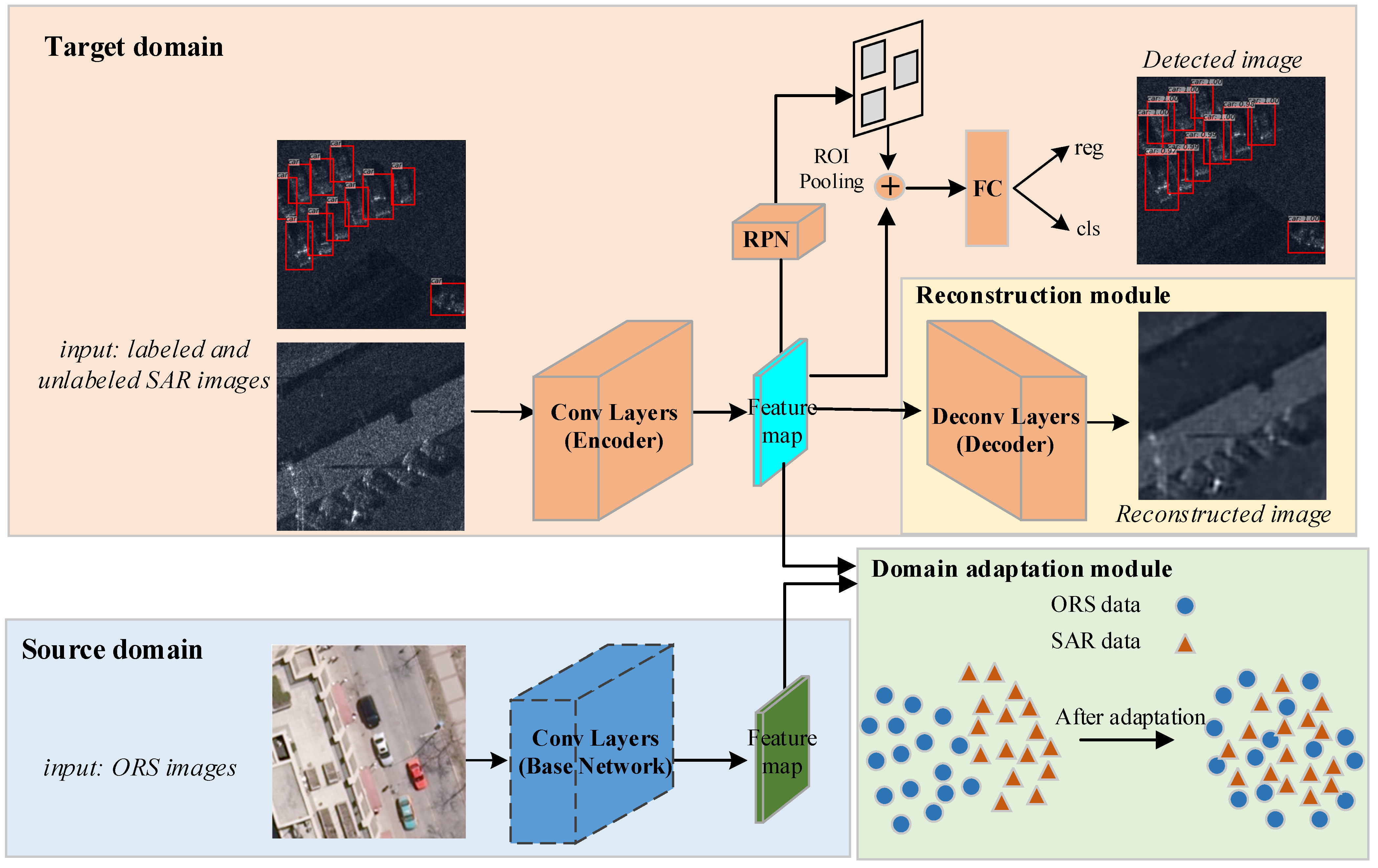
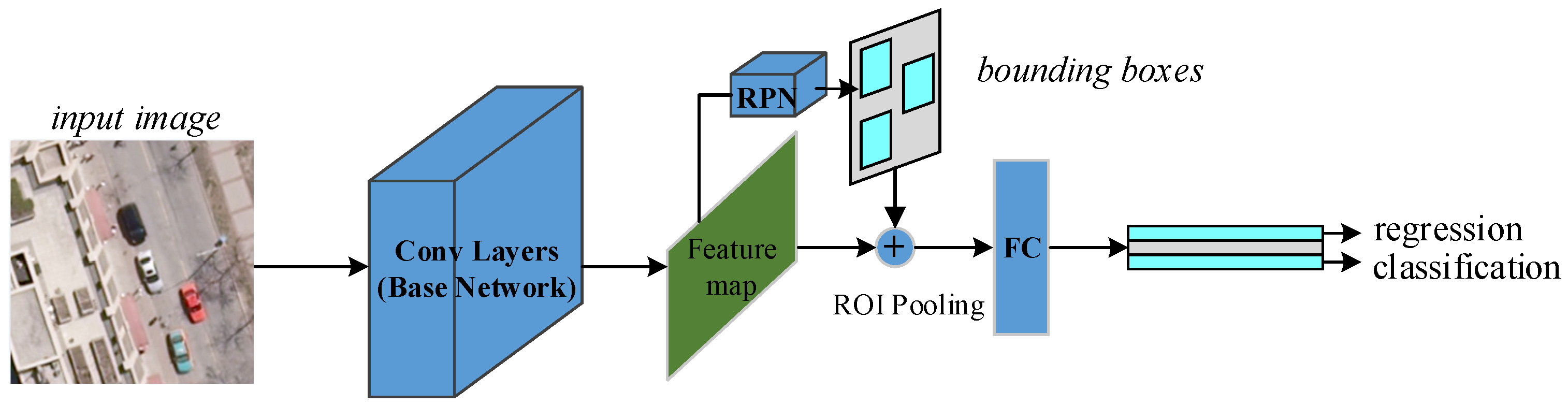
Based on faster R-CNN, a decoding module and a domain-adaptation module are introduced to develop our method. For the intuitive illustration, Figure 2 displays the whole architecture of our model. As we can see from Figure 2, there are two base networks: one is the base network (encoder) for the data from the target domain, which adopts the truncated VGG16 network with five convolution blocks consisting of thirteen convolution layers and four maxpooling layers in all; the other is the source base network that also adopts the truncated VGG16 network, and it has the fixed network parameters that are pre-trained with the labeled data from the source domain. The decoding module (decoder) has thirteen deconvolution layers and four unmaxpooling layers. In detail, the architecture of the encoder and the decoder is shown in

Table 1. Overall architecture of the encoder and decoder.

Encoder					Decoder
Layer	Size of Filter	Input/Output Channel	Stride	Feature Dimensions	Layer	Size of Filter	Input/Output Channel	Stride	Feature Dimensions
Conv1_1	3 × 3	3/64	1	512 × 512 × 64	Unconv1_1	3 × 3	64/3	1	512 × 512 × 3
Conv1_2	3 × 3	64/64	1	512 × 512 × 64	Unconv1_2	3 × 3	64/64	1	512 × 512 × 64
Pooling1	2 × 2	64/64	2	256 × 256 × 64	Unpooling1	2 × 2	64/64	2	256 × 256 × 64
Conv2_1	3 × 3	64/128	1	256 × 256 × 128	Unconv2_1	3 × 3	128/64	1	256 × 256 × 64
Conv2_2	3 × 3	128/128	1	256 × 256 × 128	Unconv2_2	3 × 3	128/128	1	256 × 256 × 128
Pooling2	2 × 2	128/128	2	128 × 128 × 128	Unpooling2	2 × 2	128/128	2	128 × 128 × 128
Conv3_1	3 × 3	128/256	1	128 × 128 × 256	Unconv3_1	3 × 3	256/128	1	128 × 128 × 128
Conv3_2	3 × 3	256/256	1	128 × 128 × 256	Unconv3_2	3 × 3	256/256	1	128 × 128 × 256
Conv3_3	3 × 3	256/256	1	128 × 128 × 256	Unconv3_3	3 × 3	256/256	1	128 × 128 × 256
Pooling3	2 × 2	256/256	2	64 × 64 × 256	Unpooling3	2 × 2	256/256	2	64 × 64 × 256
Conv4_1	3 × 3	256/512	1	64 × 64 × 512	Unconv4_1	3 × 3	512/256	1	64 × 64 × 256
Conv4_2	3 × 3	512/512	1	64 × 64 × 512	Unconv4_2	3 × 3	512/512	1	64 × 64 × 512
Conv4_3	3 × 3	512/512	1	64 × 64 × 512	Unconv4_3	3 × 3	512/512	1	64 × 64 × 512
Pooling4	2 × 2	512/512	2	32 × 32 × 512	Unpooling4	2 × 2	512/512	2	32 × 32 × 512
Conv5_1	3 × 3	512/512	1	32 × 32 × 512	Unconv5_1	3 × 3	512/512	1	32 × 32 × 512
Conv5_2	3 × 3	512/512	1	32 × 32 × 512	Unconv5_2	3 × 3	512/512	1	32 × 32 × 512
Conv5_3	3 × 3	512/512	1	32 × 32 × 512	Unconv5_3	3 × 3	512/512	1	32 × 32 × 512

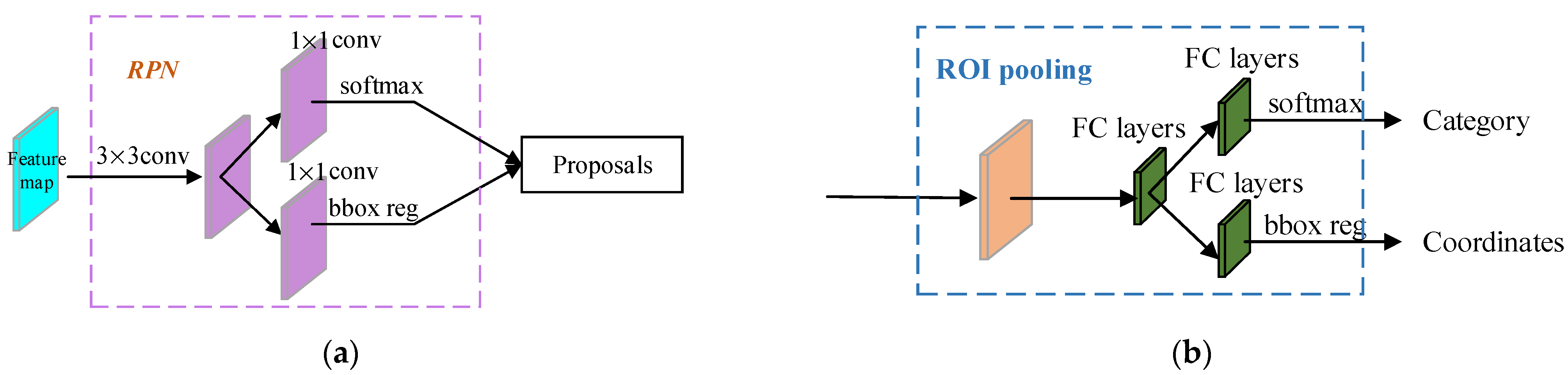
. Moreover, the RPN and ROI head networks are constructed with the same architectures as those in the original faster R-CNN [23], which are sketched in Figure 3a,b, respectively. In addition, the decoding module recovers the input sample to help learn the representative features, and the domain-adaptation module utilizes the labeled ORS images to make the features of the SAR images appear close to the discriminative features of the ORS images.

3.1.1. Decoding Module

For the large-scale unlabeled SAR images that contain abundant information on the SAR data, the proposed FDDA aims to use the unlabeled SAR images to help the model learn to make up for the lack of labels. To take advantage of the abundant unlabeled SAR images, a decoding module is first introduced to form a semi-supervised detection framework, which is inspired by the deep-convolution auto-encoder being an unsupervised model for feature extraction. The decoding module reconstructs all the labeled and unlabeled target domain data, which can exploit more information of the SAR images to learn the representative features for detection.

Since the base network (encoder) of the target domain adopts the truncated VGG16 network with five convolution blocks that are composed of thirteen convolution layers and four maxpooling layers, the decoding module (decoder) has, symmetrically, thirteen deconvolution layers and four unmaxpooling layers. In detail, the features extracted from the conv5_3 layer of the encoder are fed to the unconv5_3 layer. In the end, the output of decoder has the same size as that of the input image, with a size of $512\times 512$.

Therefore, our model extracts the features of the data from the target domain via the encoder, and the features are then fed to the decoder to reconstruct the input data. The reconstruction loss for the target domain data is written as:

$$L_{rec}=\frac{1}{N_t}{\displaystyle \sum _{i=1}^{N_t}{\Vert x_i^t-{\widehat{x}}_i^t\Vert }_2^2}$$

(10)

where ${\widehat{x}}_i^t$ is the reconstructed image of the $i\mathrm{th}$ input image $x_i^t$ from the target domain.

The proposed method contains a deep-convolutional auto-encoder architecture [12,22], which consists of the base network (encoder) and the decoding module (decoder). By reconstructing all the labeled and unlabeled SAR data, the large-scale unlabeled SAR images can be utilized to learn the representative features, which is beneficial to target detection.

3.1.2. Domain-Adaptation Module

With abundant labels, the source domain data can learn the discriminative features that are beneficial to detection. However, the target domain cannot achieve satisfactory performance with limited labels. Here, the challenge is how to utilize the source domain to help the task in the target domain. In our FDDA, we adopt the MMD constraint in our domain-adaptation module, which aims to reduce the domain discrepancy and learn the transferable features between the two related domains.

We note that there is some semantic similarity in the high-layer feature expression of the ORS images and SAR images, and thus the distributions over the high-level features can be utilized as a bridge to connect the two related domains. Specifically, to effectively reduce the domain shift, as some papers have also done [24], we use the maximum mean discrepancy (MMD):

$$L_{MMD}=\frac{1}{{\left(N_s\right)}^2}{\displaystyle \sum _{i=1}^{N_s}k\left(z_i^s,z_i^s\right)}-\frac{1}{N_s{N}_t}{\displaystyle \sum _{i=1}^{N_s}k\left(z_i^s,z_i^t\right)}+\frac{1}{{\left(N_t\right)}^2}{\displaystyle \sum _{i=1}^{N_t}k\left(z_i^t,z_i^t\right)}$$

(11)

where $z_{s_i}$ and $z_{t_i}$ are the feature maps corresponding to the inputs $x_i^s$ and $x_i^t$, and $k\left(\cdot ,\cdot \right)$ is the Gaussian kernel function $k\left(x_i^s,x_i^t\right)=e^{-{\Vert x_i^s-x_i^t\Vert }^2/\gamma }$. The input images from the two sources are both resized as $512\times 512$ and then fed to the feature extractor. Moreover, the input images of the two sources are both normalized before being inputted into the feature extractors, and thus the measurements of them are the same. Since the feature maps $Z_s$ and $Z_t$ are both the output of the conv5_3 layer in the source and target base networks, the ranges of them are the same.

In detail, the feature map $Z_s$ of the source domain data can be directly obtained via feed-forward propagation of the trained base network, which is fixed in the framework. However, the feature map $Z_t$ of the target domain data is learned with the target base network. With the MMD constraint, the features of the data from the target domain are approximated to those of the source domain. Due to the strong discriminability ability for the features of the source domain data, our method is capable of learning transferrable features that can depict the characteristics of the target domain well, using only a little labeled data. Thus, the ORS images perform as a supervisor to help improve the discriminability of the features of SAR images.

Note that the features of the data from the source domain have strong discriminative and representative ability. Our method is capable of learning transferrable features that also depict the target domain well with limited labeled data. Therefore, with the MMD-based adaptation criterion, our method can make use of the ORS images to promote target detection performance in the case of limited labeled SAR images.

3.2. Overall Objective and Optimization

As described in Section 3.1, the proposed method contains domain-adaptation and decoding modules, which, respectively, aim to borrow the information of the labeled source domain data and the large-scale unlabeled target domain data. The total objective of the constructed FDDA is expressed as:

$$L=L_{supervised}+\alpha L_{MMD}+\beta L_{rec}$$

(12)

where $L_{MMD}$ represents the adaptation loss in Equation (4), and $L_{rec}$ denotes the reconstruction loss in Equation (6); $\alpha$ and $\beta$ are the trade-off parameters that balance the interaction of the adaptation and reconstruction components, and $L_{supervised}$ is the supervised detection loss, which is the same as the loss of the traditional faster R-CNN,

$$L_{supervised}=L_{rpn}+L_{roi}$$

(13)

with $L_{rpn}$ and $L_{roi}$ denoting the RPN loss and ROI loss in the detection module for target domain data, respectively. The specific expressions of $L_{rpn}$ and $L_{roi}$ are the same as Equations (2) and (6).

To sum up, to train the FDDA, we first pre-train the faster R-CNN with ORS data to obtain the learned base network with the parameter ${\theta }_s$. Then, our goal is to minimize Equation (7) to obtain the optimized parameters of the base network for the SAR data with the parameter ${\theta }_t$, the RPN with the parameter ${\theta }_{RPN}$, the ROI fead with the parameter ${\theta }_{ROI}$, and the decoder with the parameter ${\theta }_d$. Here, we adopt the Adam optimizer [25] to optimize the objection function shown in Equation (7), which consists of the supervised detection loss, reconstruction loss, and domain-adaptation loss. Therefore, the decoder can take advantage of the unlabeled SAR data to improve the expression ability of the learned features, which further contributes to the superior detection performance. Moreover, the transferable features between two related domains can be learned by our method, and the learned features are salient, benefiting from the deep CNN and the adaptation constraint. During the test phase, one can remove the reconstruction and domain-adaptation modules, and simply use the faster R-CNN architecture with learned parameters ${\theta }_t$, ${\theta }_{RPN}$, and ${\theta }_{ROI}$ to obtain the detection results via feed-forward propagation.

4. Experimental Results and Analysis

To evaluate the detection performance of our method, this section presents some experimental results. The description of the measured datasets and some experimental settings are firstly introduced. Then, some results, based on two domain adaptation scenarios, are shown.

4.1. Description of the Datasets and Experimental Settings

In the following, some experiments are conducted based on two SAR image datasets and one ORS image dataset. The SAR image datasets include the miniSAR dataset [26] and the FARADSAR dataset [27], and the ORS images come from the Toronto dataset [28].

The miniSAR and FARADSAR datasets were, respectively, acquired by U.S. Sandia National Laboratories in 2005 and 2015, and the resolution of SAR images in the two datasets is 0.1 m × 0.1 m. The miniSAR dataset contains nine images, and the sizes of them are 1638 × 2510 pixels; seven images were selected as the training dataset and the rest were used for the test. The FARADSAR dataset contains 106 images with sizes ranging from 1300 × 580 to 1700 × 1850 pixels, where 78 images were used as the training data and the remaining 28 images were taken as the test data. In the Toronto dataset, the ORS images cover the city of Toronto, in which the ORS images have a spatial resolution of 0.15 m and a color depth of 24 bits per pixel (RGB). There is a large image in the Toronto dataset, with a size of 11,500 × 7500 pixels, and it is segmented into several subareas, in which 13 and 10 subareas are, respectively, taken as the training and test datasets.

In

Table 2. The parameters of the miniSAR, FARADSAR, and Toronto datasets.

System Characteristics	miniSAR	FARADSAR	Toronto
Incidence angle	61–64	56–61	-
Location	Kirtland Air Force Base	The University of New Mexico	The city of Toronto, Canada
Scenes	Golf course, helicopter park, baseball field, etc.	Dense urban buildings	Dense urban buildings under sunny weather
Time	2005	2015	2016
Resolution	0.1 m × 0.1 m	0.1 m × 0.1 m	0.15 m × 0.15 m

, we list the parameters, including the incidence angles, location, scene, time, and resolution, for the above three datasets. As we can see from Table 2, the scenes of the three datasets are very complex. Moreover, as shown in the second column of Table 2, there exists a small variation of the incidence angle for the miniSAR dataset, i.e., only from 61 degrees to 64 degrees. Thus, in the experiments on the miniSAR dataset, the variation of the incidence angle has minor impacts on the geometry variation for the targets in the SAR images. 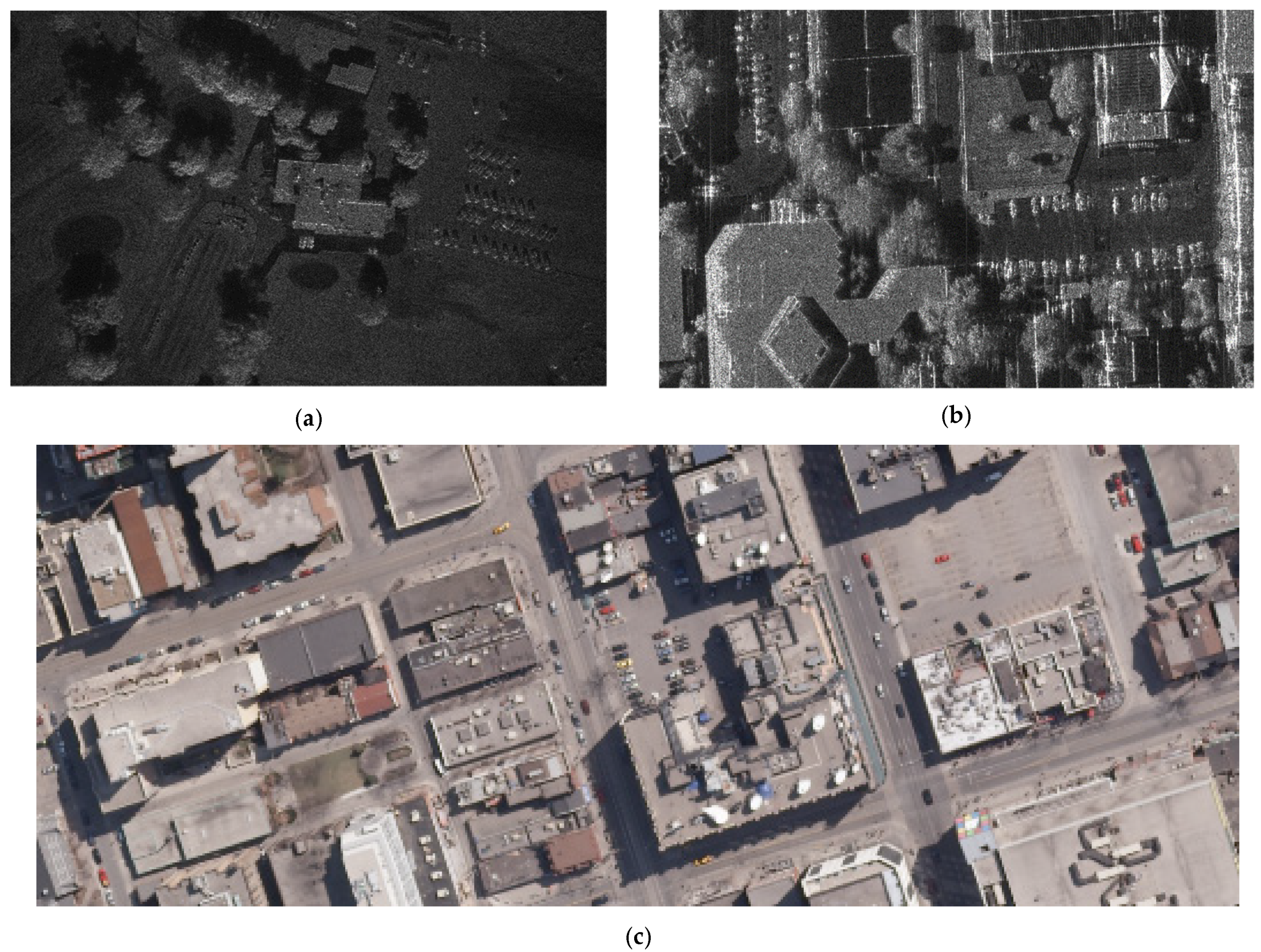Analogously, the third column of Table 2 shows that the incidence angles of the FARADSAR dataset also have a small variation range, only from 56 degrees to 61 degrees, illustrating the minor impacts on the SAR targets in the experiments with the FARADSAR dataset. In detail, we will show some image samples to provide a more intuitional illustration. In Figure 4, we present images samples for the two SAR datasets. Figure 4a shows a sample in the miniSAR dataset that covers the scene of Tijeras Arroyo Golf Course in the Kirtland Air Force Base with some of the targets (cars) locating on the road, close to the trees, under the buildings, and so on. Analogously, Figure 4b presents an image of the FARADSAR dataset, which is the scene of the Advisement and Enrichment Center at the University of New Mexico. Moreover, we present an image from the Toronto dataset in Figure 4c, which covers the complex city street scenes of the Toronto city. In the miniSAR and FARADSAR datasets, the SAR targets contain cars, buildings, trees, grasslands, concrete grounds, roads, vegetation, golf courses, baseball fields, helipads, and so on. Therefore, the number of all the SAR targets is about 10. Up to now, the miniSAR and FARADSAR datasets are the most complex SAR image datasets that we can find and that are publicly available. It makes sense to verify the effectiveness of our method on datasets with complex scenes.

In the above three datasets, the size of the images is too large to be directly used as the network input. Thus, we first crop the original images in the three datasets into many sub-images with sizes of 300 × 300, and then these sub-images can be used to train the network. Moreover, in our model, these sub-images need to be resized to 512 × 512 to input them into the base network. Analogously, the original test images are also cropped into some sub-images, with sizes of 300 × 300, by sliding the window repeatedly, and we set the sliding window repetition to 100 pixels. After detection for the test sub-images, these detected images are then restored to the big SAR images with the same size as those in the datasets. In the restoration process, we apply the non-maximum suppression (NMS) deduplication for the detection results in the sub-images to attain the final results.

For the miniSAR dataset, there are 110 training samples, and there are 330 training samples for the FARADSAR dataset. To validate the detection results of the semi-supervised detection network in the case of limited labels, in this paper, the percentage of labels in the training dataset is set to 30%. The 30% labeled training samples are randomly selected six times from all training samples, and the mean and variance over the six random experiments are taken as the final test result. Moreover, the established domain-adaptation scenarios include adaptations (1) from the Toronto dataset to the miniSAR dataset ($T\to M$), and (2) from the Toronto dataset to the FARADSAR dataset ($T\to F$). In our experiments, the original faster-RCNN is adopted as the baseline detection model.

In the objective function, the weights of the MMD and the reconstruction terms, i.e., $\alpha$ and $\beta$, are set to $0.1$ and $1$, respectively. The Adam algorithm is adopted for model optimization, and the learning rate is 5 × 10⁻⁵; the decay is set to 0.1 and the momentum is set to 0.5. Moreover, the Gaussian kernel parameter $\gamma$ is set to 0.5 in our method. Our method is implemented with Pytorch [29].

4.2. Evaluation Criteria

To comprehensively present the quantitative results of the different methods, we adopt several widely used criteria, including precision, recall, and F1-score. In the following, we present the formulas of these criteria as:

$$Precision=\frac{TP}{TP+FP}$$

(14)

$$Recall=\frac{TP}{FP+TN}$$

(15)

$$F1-score=\frac{2\times Precision\times Recall}{Precision+Recall}$$

(16)

where TP denotes the number of correctly detected targets, FP denotes the number of false alarms, and FN represents the number of missing alarms. The precision indicates the fraction of true positive results over all the detected results, and the recall shows the fraction of true positive results over ground-truths. The F1-score presents the harmonic mean between the precision and recall, and it is taken as the main referenced criterion for showing the detection performance.

4.3. Results on the MiniSAR Dataset

The experiments on the miniSAR dataset are conducted in this section, and the domain adaptation from the Toronto dataset to the miniSAR dataset ($T\to M$) is adopted in our method. Firstly, the source domain data, i.e., the Toronto dataset, is utilized for faster R-CNN training, which has gained superior detection performance on the test images of the Toronto dataset, with the F1-score being 0.9260. Therefore, the Toronto dataset contains abundant labeled training data that can be used to help SAR target detection.

4.3.1. Detection Performance Comparison with Other Methods

In this subsection, we evaluate the detection performance of our method on the miniSAR dataset, comparing it to some related methods.

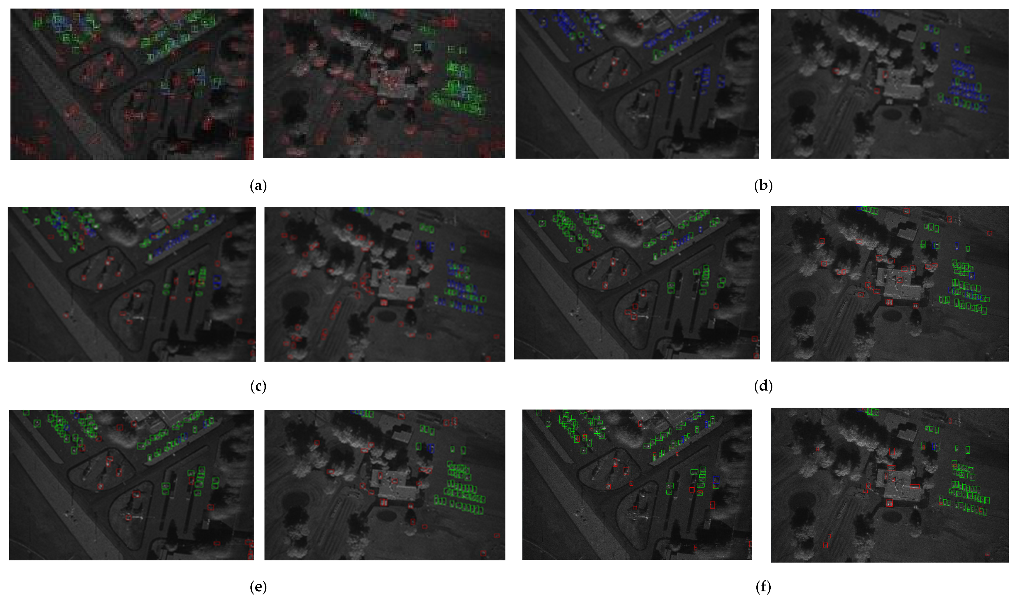
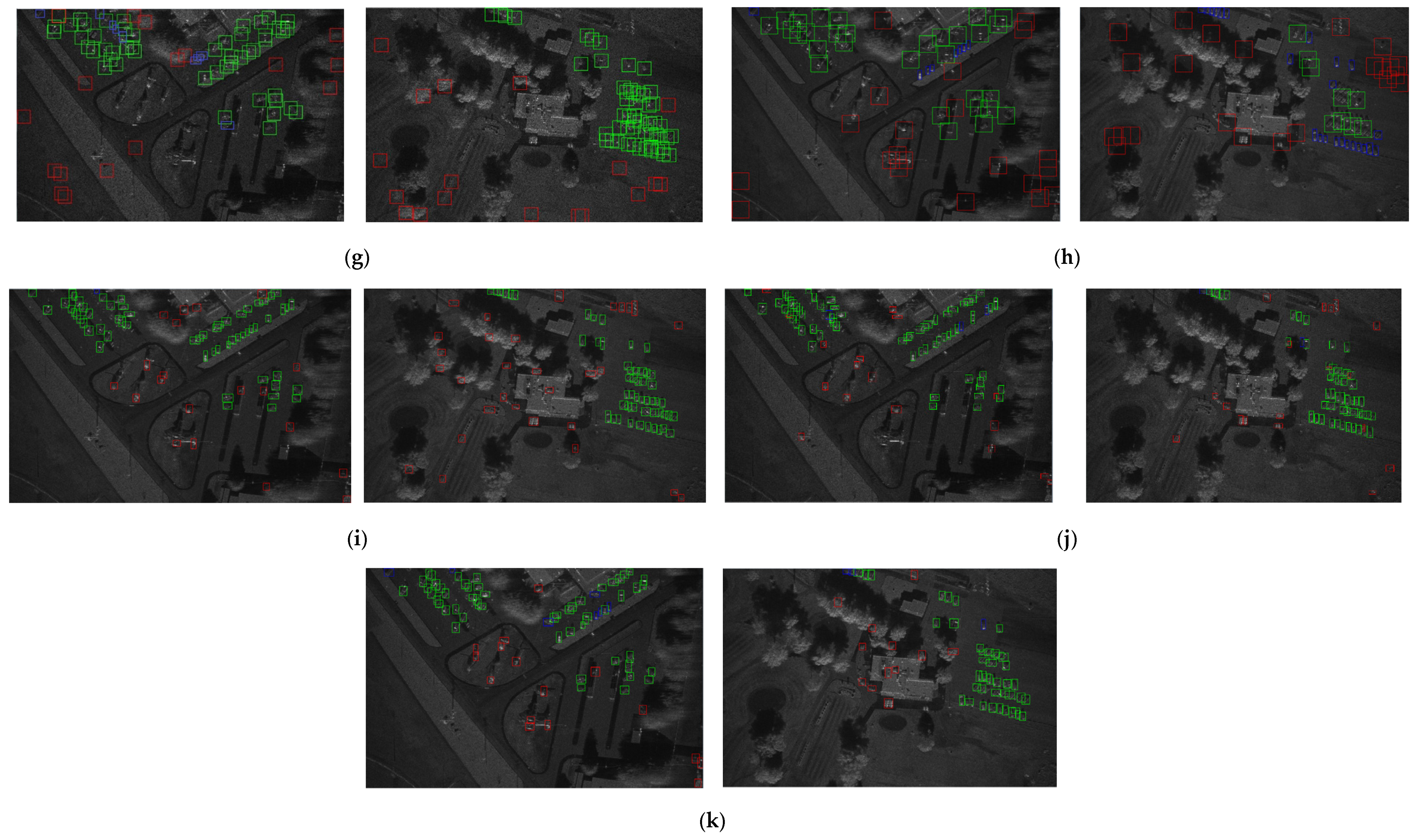
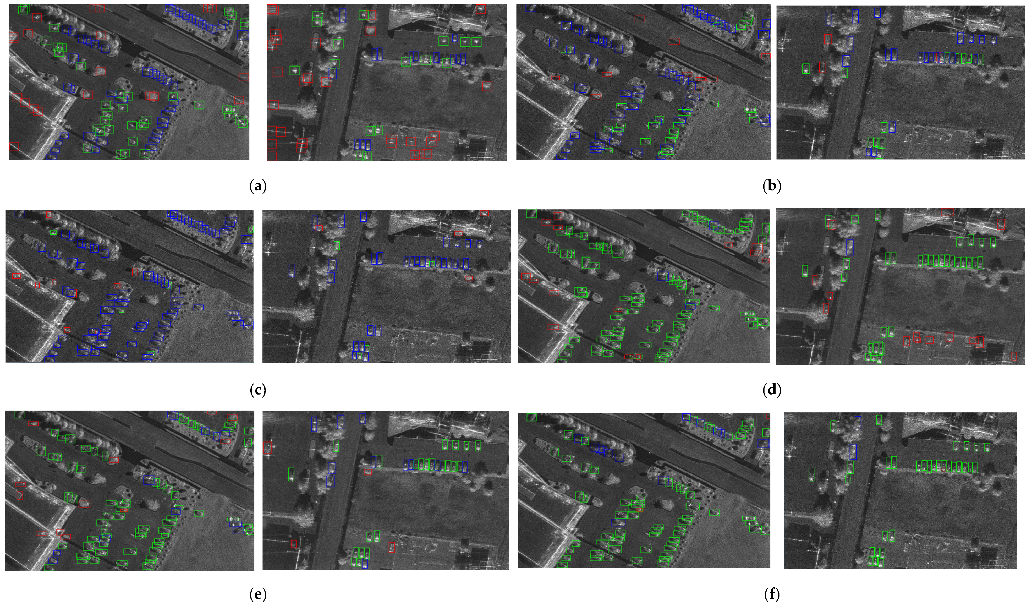
In Figure 5, we present the detection results of two test images obtained by the proposed method, as well as some comparisons. As we can see from Figure 5a, the detection results of the Gaussian-CFAR contain a lot of false alarms and some missing alarms; since the Gaussian-CFAR is an unsupervised method, the performance is restricted when the SAR scenes are complex. In addition, Figure 5b,c show the detection results of the DAF and HTCN, respectively, and there are lots of missing alarms and false alarms. Since the domain gap between the Toronto and miniSAR datasets is large, such unsupervised domain-adaptation methods, i.e., DAF and HTCN, cannot perform well. Figure 5d illustrates that the labels of the SAR images contribute to the better detection performance of faster R-CNN than unsupervised methods. Moreover, as shown in Figure 5e, the DAPN benefits from the multiple scales of feature-fusion and from the attention mechanism and thus performs better than faster R-CNN. Figure 5f displays the results of YOLOv5 [30], which performs well on the SAR data, since YOLOv5 benefits from the anchor-free, DropBlock, and label-smoothing mechanism. Figure 5g,h show the results of the Rosenberg’s method and the Zhang’s method, respectively, which both have a large number of false alarms. They are self-learning-based methods and tend to select the wrong clutter as the target, thereby causing lots of false alarms. In addition, Figure 5i presents the results of STAC. Comparing to the results of faster R-CNN, STAC can effectively reduce the missing alarms but brings more false alarms. Since the pseudo-labels for the unlabeled data may be not correct, STAC will regard the clutter as the target and lead to more false alarms. Moreover, in Figure 5j, the Soft Teacher [31] benefits from the data augmentation and a soft-teacher mechanism to improve the accuracy of the pseudo-labels, which has gained promising detection results. Comparing to the related methods, the results of our proposed FDDA shown in Figure 5k have much fewer missing and false alarms. With the domain adaptation from the Toronto images to the miniSAR images, the proposed method could learn much more representative features for detection, and the decoding module also helps learn the representative features of the SAR data, thus leading to a much better detection performance. Furthermore, as for two of the test images, the quantitative detection results of the proposed method and some comparisons are displayed in

Table 3. The detection methods of different methods on the miniSAR dataset.

$\mathit{T}\to \mathit{M}$	Supervision Mode	Domain Adaptation	Target Amounts	Missing Alarms	False Alarms	Precision	Recall	F1-Score
Gaussian-CFAR	Unsupervised	No	123	17	176	0.3868	0.8618	0.5339
DAF		Yes		100 ± 2	11 ± 3	0.6744 ± 0.0171	0.1890 ± 0.0195	0.2950 ± 0.0217
HTCN		Yes		79 ± 5	23 ± 4	0.6406 ± 0.0194	0.3577 ± 0.0221	0.4591 ± 0.0231
Faster R-CNN	Fully supervised	No		12 ± 5	41 ± 7	0.7097 ± 0.0256	0.9036 ± 0.0426	0.7939 ± 0.0102
DAPN		No		10 ± 2	39 ± 2	0.7334 ± 0.0072	0.9148 ± 0.0226	0.8180 ± 0.0085
YOLOv5		No		7 ± 2	40 ± 3	0.7402 ± 0.0183	0.9472 ± 0.0057	0.8310 ± 0.0138
Rosenberg’s method	Semi- supervised	No		11 ± 1	62 ± 4	0.6288 ± 0.0035	0.9126 ± 0.0108	0.7652 ± 0.0130
Zhang’s method		No		48 ± 20	28 ± 19	0.5631 ± 0.0162	0.6098 ± 0.1644	0.5622 ± 0.0189
STAC		No		1 ± 2	50 ± 6	0.6914 ± 0.0280	0.9919 ± 0.0115	0.8148 ± 0.0148
Soft Teacher		No		5 ± 2	35 ± 3	0.7667 ± 0.0111	0.9593 ± 0.0081	0.8523 ± 0.0067
Proposed FDDA		Yes		9 ± 2	27 ± 4	0.8169 ± 0.0221	0.9187 ± 0.0137	0.8592 ± 0.0048

. Note that the Gaussian-CFAR is directly applied to the test images, and there is no randomicity about the method. Thus, there is no mean and variance of results for the Gaussian-CFAR. Since the performance of CFAR algorithms depend on the detection threshold, the results of CFAR algorithms are made best by setting different thresholds. As we can see from Table 3, the proposed method has higher detection precision and recall, which leads to higher F1-scores. Thus, Table 3 also validates that our method obtains much better detection performance than the comparisons on the miniSAR dataset.

4.3.2. Model Analysis

• Ablation Study

In our method, the baseline model is faster R-CNN, and we incorporate the decoding and domain-adaptation modules to achieve superior semi-supervised SAR target detection performance. To analyze the effect of the two modules in the proposed method, the ablation study is conducted in the following, and

Table 4. Ablation results of our method on the miniSAR dataset.

$\mathit{T}\to \mathit{M}$	Components		Target Amounts	Missing Alarms	False Alarms	Precision	Recall	F1-Score
	MMD	Decoder
Faster R-CNN	✕	✕	123	12 ± 5	41 ± 7	0.7097 ± 0.0256	0.9036 ± 0.0426	0.7939 ± 0.0102
Ours	✕	✓		9 ± 2	34 ± 6	0.7660 ± 0.0289	0.9214 ± 0.0142	0.8362 ± 0.0162
	✓	✕		11 ± 5	36 ± 6	0.7508 ± 0.0223	0.9052 ± 0.0441	0.8198 ± 0.0088
	✓	✓		9 ± 2	27 ± 3	0.8169 ± 0.0221	0.9187 ± 0.0137	0.8592 ± 0.0048

shows the quantitative experimental results with 30% labeled training samples of the miniSAR dataset. As shown in Table 4, the decoding and domain-adaptation modules both devote attention to fewer missing and false alarms, and have higher precision, recall, and F1-scores. In the proposed method, the decoding module makes use of the unlabeled training samples to exploit much more useful information for detection, and the MMD constraint helps learn some features depicting the target domain data well. In this way, our method gains much better detection performance than the baseline model, confirming the positive effect of the decoding and domain adaptation modules in our method.

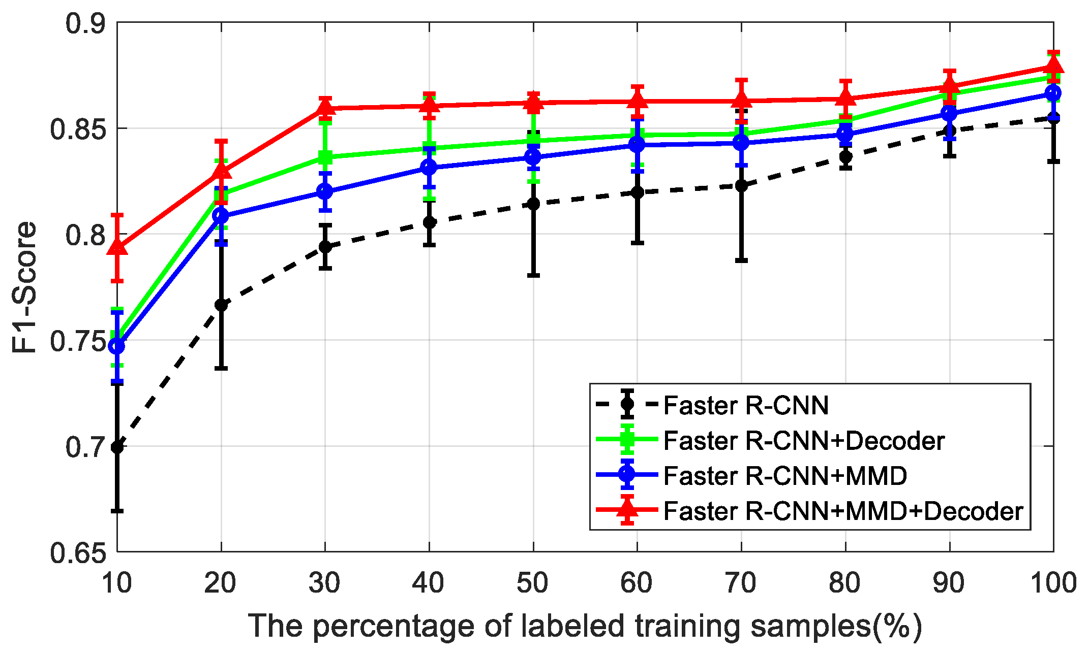
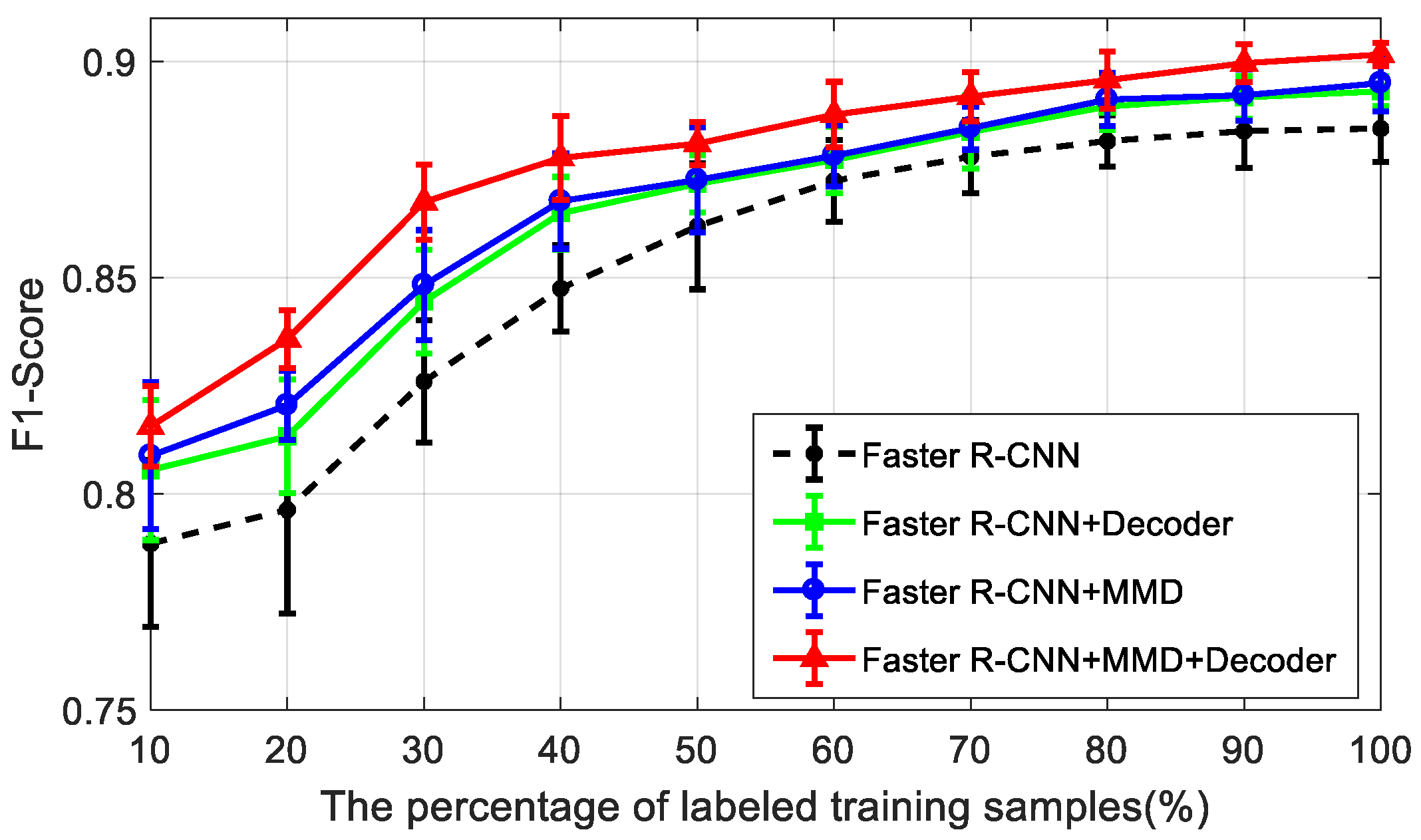
Furthermore, the ablation experimental results of the mean and variance of the F1-scores with different percentages of labeled training samples, from 10% to 100%, are presented in Figure 6. The faster R-CNN is the baseline model that is taught only with the labeled training samples. In Figure 6, with the increase of the labeled training samples, the F1-scores of all these methods gradually increase. Comparing to faster R-CNN, other models with a decoding module or a domain-adaptation module have shown better results with higher mean and lower variance of the F1-scores—especially our model, which features both modules. Particularly, if the percentage of the labeled training samples is smaller, the performance promotion of the decoding and domain-adaptation modules is more obvious. Therefore, our semi-supervised method takes advantages of the decoding and domain-adaptation modules to attain much better detection performance than the baseline faster R-CNN in the case of limited labeled SAR images.

• Reconstruction performance

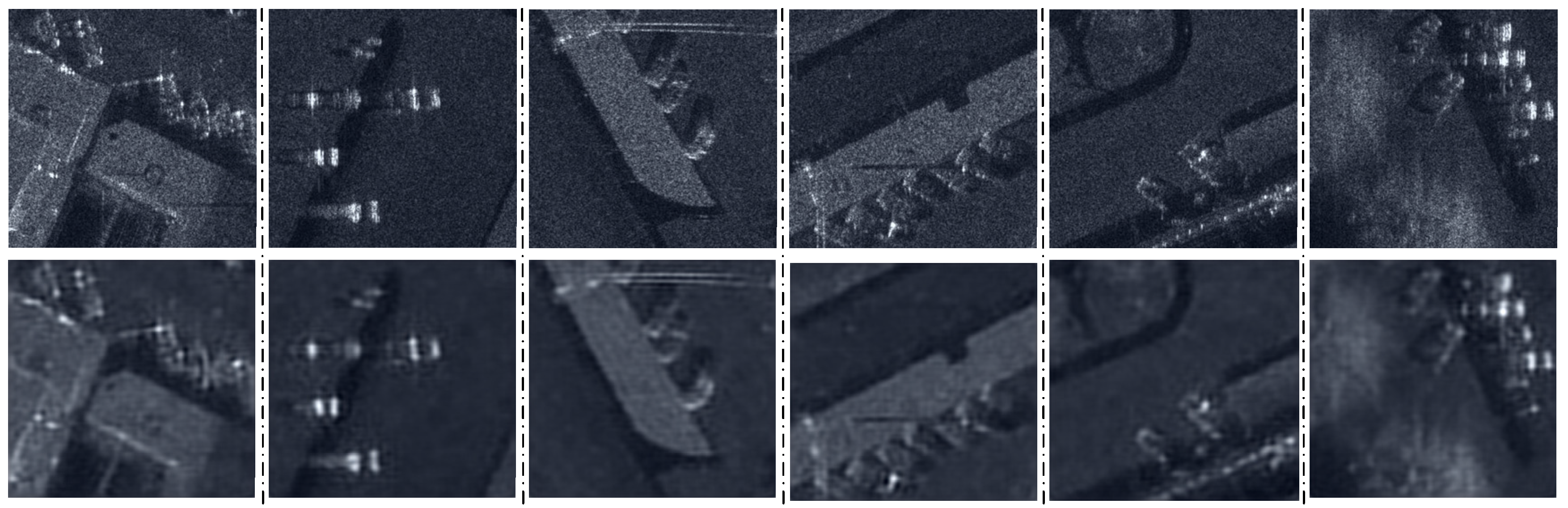
The proposed semi-supervised method is taught with the training images, in which only 30% of the data contain labels and the rest are unlabeled. For the unlabeled miniSAR images, they are recovered via the decoding module. To show the reconstruction effect of the decoding module, in Figure 7, we present the original and recovered samples. As we can see from Figure 7, comparing to the original miniSAR chips in the first row, the recovered samples in the second row retain the target (car) and background information, which shows that the convolutional autoencoder branch in our method performs well on recovering the original input samples. Thus, the proposed method can take advantage of the large-scale unlabeled SAR images for exploring more information of the miniSAR dataset, which is helpful for SAR target detection.

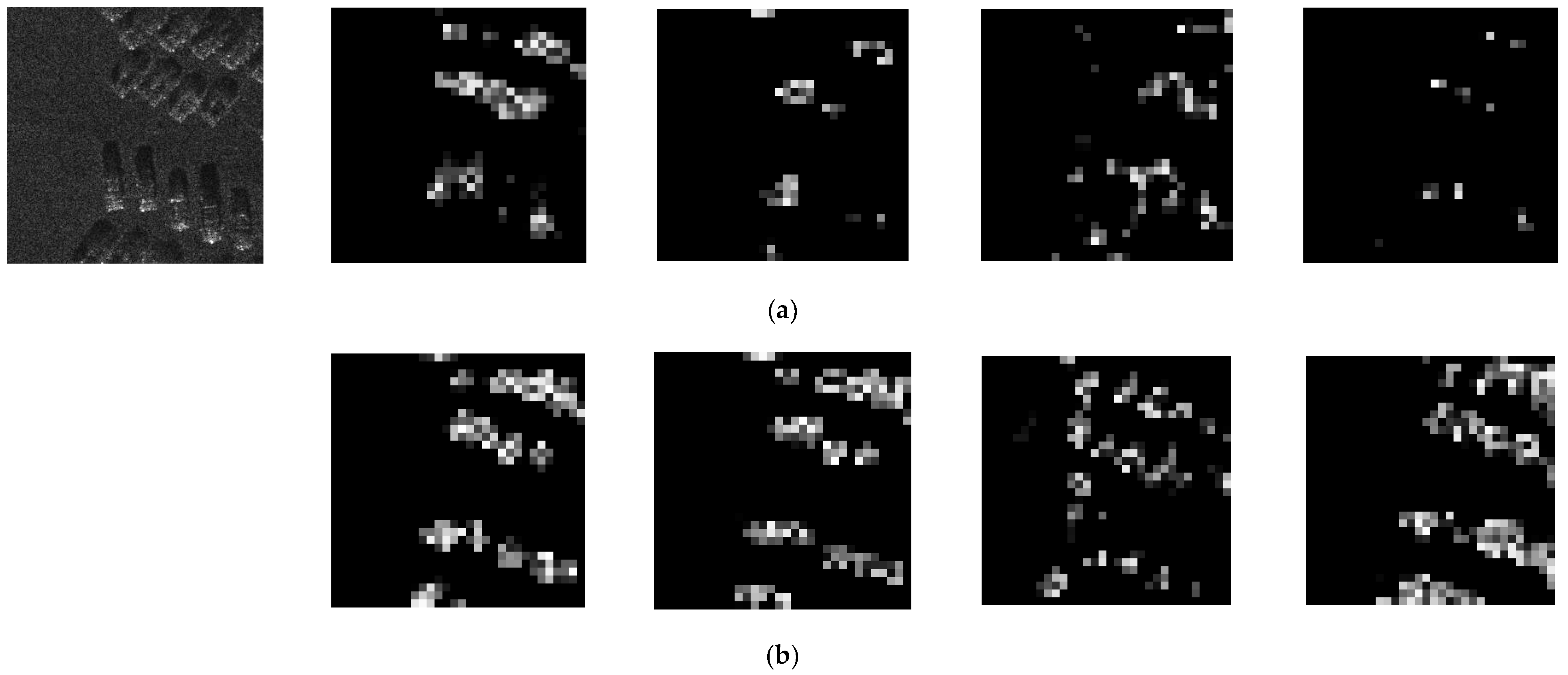
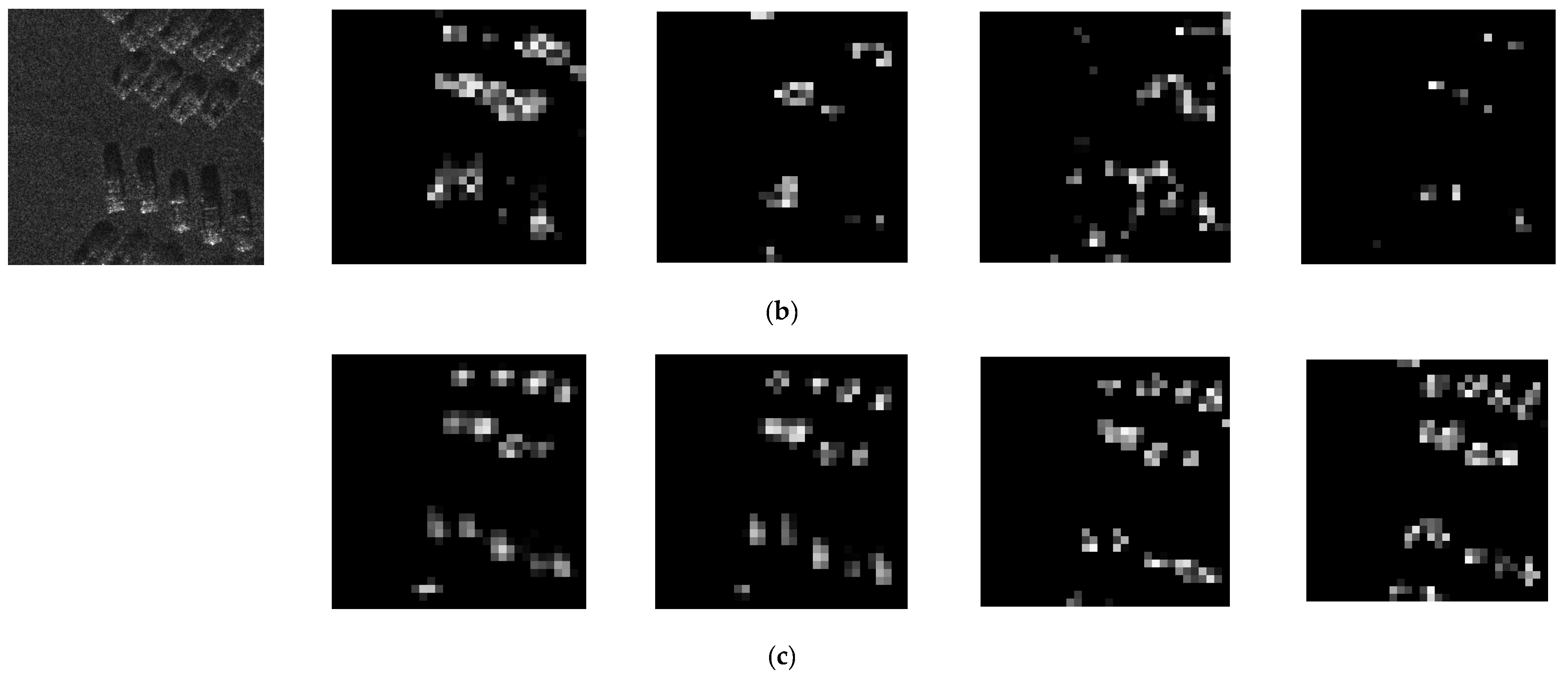
To illustrate the effect of the decoding module on the feature extraction, we compare the feature maps in the conv5_3 layer gained with the original faster R-CNN and the faster R-CNN with the decoder. Here, we take four feature maps from four channels as examples and show the results in Figure 8. The first image in Figure 8a presents an original test chip in the miniSAR dataset, and the other images in Figure 8a are its feature maps obtained by the original faster R-CNN, which are very fuzzy and omit some important information about the targets. Figure 8b shows the four corresponding feature maps via the faster R-CNN with the decoder, and almost all of the target information is covered in the feature maps. Since there are a small number of labeled training images, the feature maps obtained by the faster R-CNN have limited representative ability. By incorporating the decoding module into the faster R-CNN, the model can make use of a large number of unlabeled SAR images to exploit representative features to cover the target information, thus improving the expression capability of the feature maps for the targets in the SAR images.

• Domain adaptation performance

Though the ORS and SAR images capture different scenes, for the target of interest, such as the car, there is some semantic similarity in the high-layer feature expression. The well-learned features of the ORS images can be used to help the feature extraction of the SAR data via our adaptation method, and the features of the SAR data can be further utilized for target detection. In the following, we conduct some experiments to give a clear illustration of the interpretation of the transferred knowledge of the ORS images and show the intuitionistic effects on the SAR images.

To analyze the domain-adaptation effect with an intuitive visualization, the original features in the multidimensional space are mapped onto a two-dimensional space by the means of t-distribution stochastic neighbor embedding (t-SNE) [2]. In the following, we present the t-SNE visualization results for features of samples from the Toronto and miniSAR datasets. In the miniSAR dataset, the training chips have 110 samples, while the training chips in Toronto datasets have 2600 samples. Thus, 110 examples are randomly chosen from the Toronto dataset. The features of the SAR and ORS images are, respectively, extracted by the source and target base networks; then, the features are jointly projected onto a common two-dimensional space by the means of t-SNE. 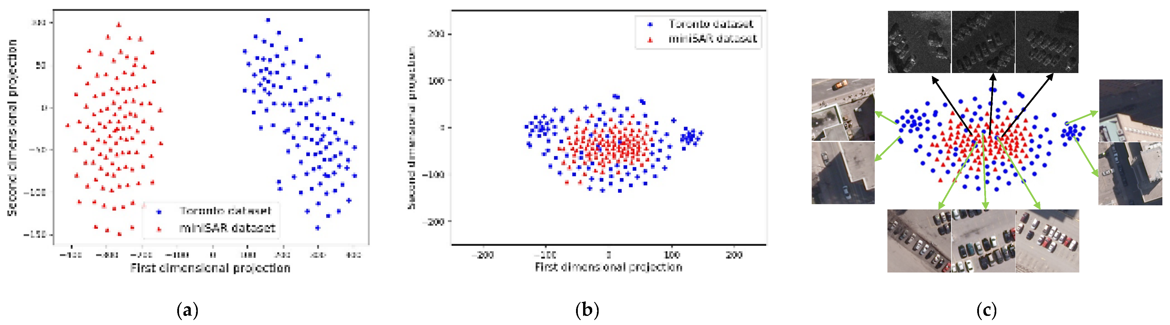In Figure 9, we present the projection results of the features, and Figure 9a,b present the feature distributions before and after adaptation, respectively. In detail, Figure 9a shows that the features between the SAR and ORS images have clear margins, which illustrates the great domain discrepancy between the features of the SAR and ORS image domains. Moreover, with the MMD adaptation, the features of the SAR and ORS images distribute closely to each other, showing that the feature distribution is aligned and that the domain shift is greatly reduced. Since there is great discrepancy between the ORS and SAR images, the adaptation constraint cannot totally mix the SAR and ORS images to be uniformly distributed. For a clear illustration, corresponding to the feature of Figure 9b, we show some image examples in Figure 9c, where the black line arrows and green line arrows indicate the miniSAR data and Toronto data, respectively. In Figure 9c, for the samples distributed in the center, the targets and backgrounds of the SAR images are similar to those of the ORS images. Nevertheless, as for the samples displayed in the left column and right column of Figure 9c, these ORS images are far away from the SAR data and have very different scenes from that of the SAR data, such as cars under shadows, close to buildings, and so on. To a certain degree, the MMD performs well on constraining the feature-distribution of the data from the two domains to be close to each other, but the great discrepancy makes it hard to be as well-proportioned as possible.

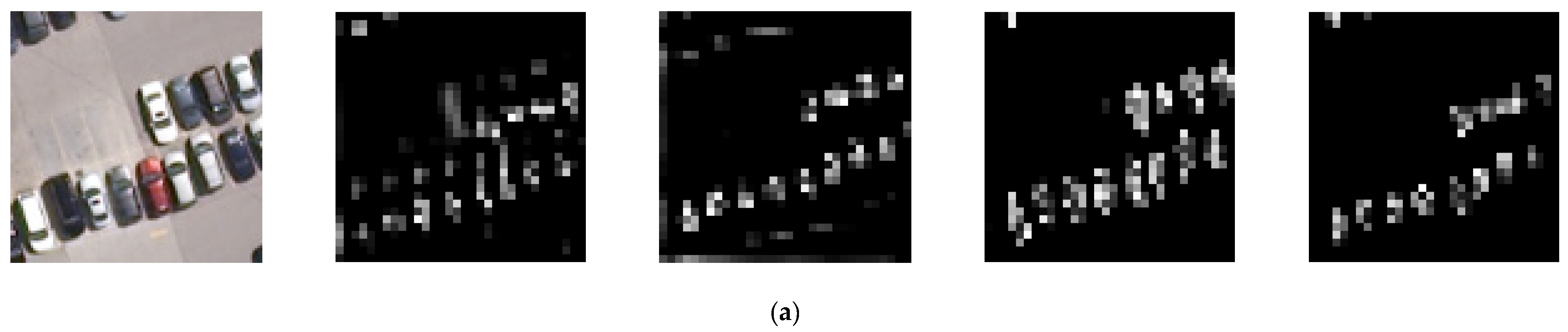
Furthermore, we conduct some experiments to show the effect of the ‘transferred knowledge’ of the ORS images to the feature maps of the SAR images. For clear illustration, we randomly choose an image chip of a test image in the Toronto dataset, which is displayed in Figure 10a. Correspondingly, the feature maps of four channels in the conv5_3 layer for the chip in the first column of Figure 10a are presented in the other four columns of Figure 10a. Since the ORS data has abundantly labeled training samples, the highlight area of the feature maps can precisely locate the targets, which further validates the superior performance of faster R-CNN for the ORS data. Analogously, the first image in Figure 10b shows the image chip of a test image in the miniSAR dataset, and the other columns of Figure 10b are the four feature maps obtained via the baseline faster R-CNN. Correspondingly, Figure 10c presents the four feature maps obtained via the faster R-CNN MMD adaptation. As we can see from Figure 10b, the feature maps are fairly fuzzy and nearly cannot precisely indicate the location of the targets, indicating a limited detection performance. Comparing to the results in Figure 10b, in Figure 10c, the results obtained via faster R-CNN with the MMD constraint perform much better with precise locations for the targets. Since the domain-adaptation module can transfer the abundant knowledge of the ORS images to help the feature-extraction of the SAR images, the discriminative features of the SAR images can be learned to depict the target characteristics precisely.

4.4. Results on the FARADSAR Dataset

We then show the detection results of our method on the FARADSAR dataset. Here, the domain adaptation scenario is from the Toronto dataset to the FARADSAR dataset ($T\to F$). In the following, we present the detection results on the FARADSAR dataset obtained by our method and some related methods.

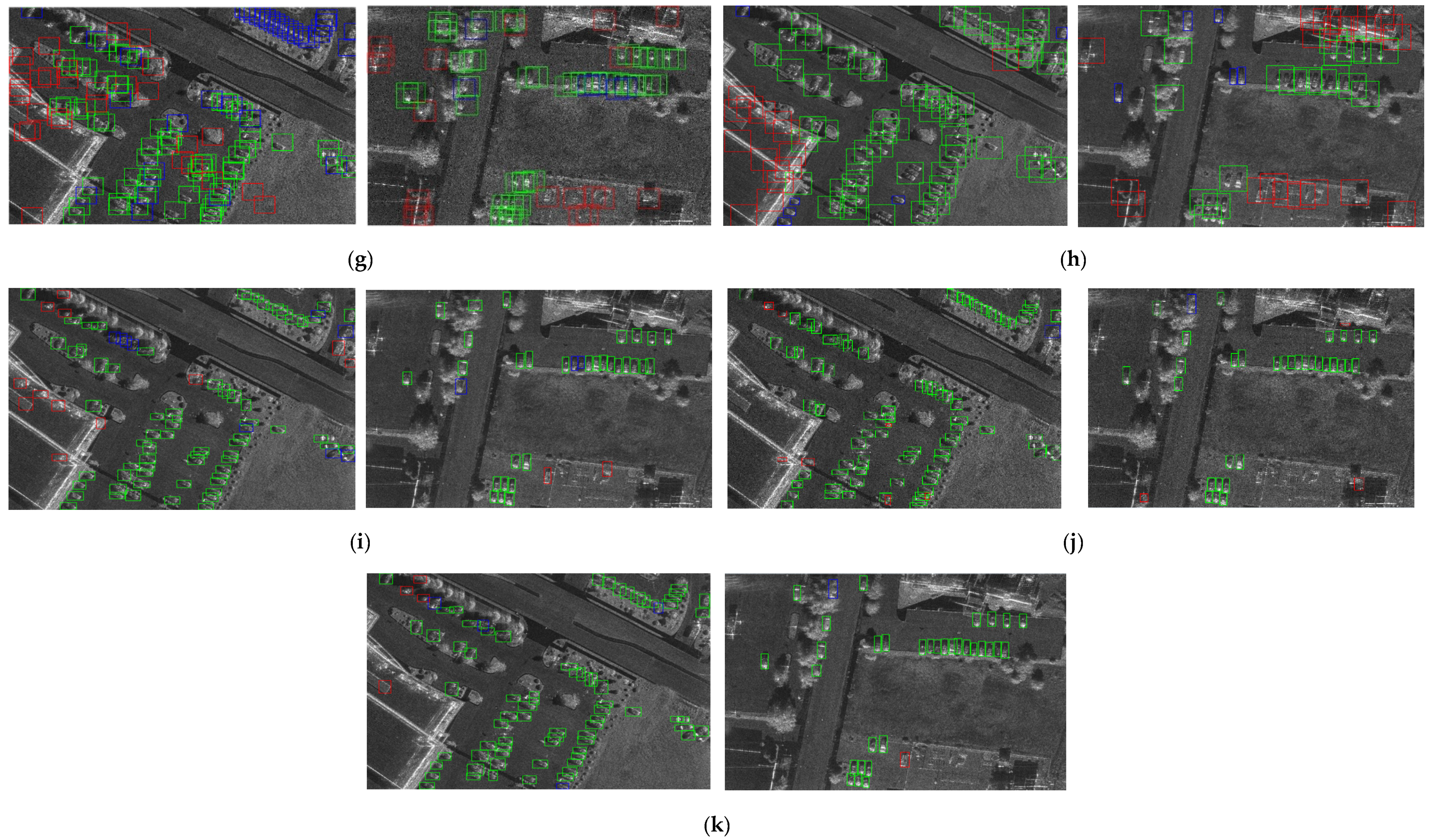
In Figure 11, we display the detection results of two test images from the FARADSAR dataset obtained by our method, as well as some comparisons. Due to the complex SAR scenes in the FARADSAR dataset, the detection results of the Gaussian-CFAR are restricted, with many false alarms and missing alarms. The unsupervised domain-adaptation methods, including DAF and HTCN, still cannot perform well on the FARADSAR images, for there are great domain shifts between the Toronto and FARADSAR images that cause a great performance degradation. In addition, the baseline faster R-CNN gains promising detection performance on the FARADSAR dataset, while YOLOv5 [30] achieves better results that benefit from the anchor-free, DropBlock, and label-smoothing mechanism. For the self-learning-based semi-supervised methods, i.e., Rosenberg’s method and Zhang’s method, the clutter in the SAR scenes of the FARADSAR dataset are easily regarded as the targets; thus, the results of the two methods have many false alarms. Moreover, STAC utilizes the pseudo-labels of the unlabeled images and the data-augmentation strategy to retrain the model, which achieves fewer missing alarms but more false alarms than faster R-CNN. The Soft Teacher [31] is still effective on the FARADSAR dataset, by means of a soft-teacher mechanism that produces accurate pseudo-labels for the unlabeled data. However, our method gains better results than the comparisons, with fewer missing and false alarms, since the decoding and adaptation modules can use the unlabeled images and the ORS images to promote detection results. Furthermore, for a clearer illustration, the quantitative detection results are illustrated in

Table 5. The target detection results of different methods on the FARADSAR dataset.

$\mathit{T}\to \mathit{M}$	Supervision Mode	Domain Adaptation	Target Amounts	Missing Alarms	False Alarms	Precision	Recall	F1-Score
Gaussian-CFAR	Unsupervised	No	691	368	823	0.2813	0.4671	0.3512
DAF		Yes		448 ± 12	119 ± 23	0.6405 ± 0.0166	0.3252 ± 0.0119	0.4315 ± 0.0157
HTCN		Yes		484 ± 18	243 ± 16	0.4228 ± 0.0142	0.2741 ± 0.0124	0.3304 ± 0.0214
Faster R-CNN	Fully supervised	No		54 ± 8	209 ± 39	0.7482 ± 0.0231	0.9219 ± 0.0145	0.8260 ± 0.0142
DAPN		No		89 ± 14	144 ± 19	0.8000 ± 0.0137	0.8509 ± 0.0191	0.8341 ± 0.0046
YOLOv5		No		89 ± 6	113 ± 11	0.8373 ± 0.0123	0.8712 ± 0.0082	0.8538 ± 0.0025
Rosenberg’s method	Semi- supervised	No		185 ± 12	325 ± 23	0.4506 ± 0.0067	0.7325 ± 0.0108	0.5580 ± 0.0059
Zhang’s method		No		142 ± 26	917 ± 35	0.3744 ± 0.0163	0.7945 ± 0.0208	0.5090 ± 0.0129
STAC		No		39 ± 6	220 ± 18	0.7477 ± 0.0146	0.9435 ± 0.0082	0.8343 ± 0.0088
Soft Teacher		No		50 ± 8	157 ± 6	0.8035 ± 0.0036	0.9276 ± 0.0112	0.8611 ± 0.0062
Proposed FDDA		Yes		49 ± 6	141 ± 12	0.8184 ± 0.0135	0.9291 ± 0.0088	0.8681 ± 0.0129

, from which the same conclusions as Figure 11 can be obtained. Thus, the results in Figure 11 and Table 5 both validate that our method outperforms the comparisons on the FARADSAR dataset.

To show the effectiveness of the proposed semi-supervised method in different cases of limited labels, we conduct the experiments with different percentages of labeled training samples on the FARADSAR dataset. The mean and variance results of the F1-scores with different percentages of labels, from 10% to 100%, are shown in Figure 12. As displayed in Figure 12, when the percentage of labels increases, the detection performance of different models gradually improves and becomes steady when the percentage of labels is large enough. Moreover, comparing to the baseline model (faster R-CNN), the decoding module (decoder) and domain-adaptation module in our method both have a positive impact on the detection results, with a higher mean and lower variance of the F1-score. Notably, when the percentage of labels is smaller, the performance improvement of the models with the decoder and domain-adaptation modules is more obvious. Therefore, the ablation study results on the FARADSAR dataset validate the effectiveness of the decoder and MMD for utilizing the large-scale unlabeled SAR images to promote the semi-supervised SAR target detection performance.

5. Conclusions

This paper focuses on the construction of an improved faster R-CNN for semi-supervised SAR target detection by taking advantages of a decoding module and a domain-adaptation module. Our method introduces the decoding module to explore more information of SAR images by reconstructing all labeled and unlabeled images, which is beneficial to learn the representative features for target detection. Moreover, by adopting the domain-adaptation module, our method can utilize the unlabeled SAR images to further promote the discriminability of the features with the assistance of labeled ORS images, and thus, the features can depict the targets precisely and are useful for target detection. Our method is an end-to-end framework that is learned by jointly optimizing the detection loss, reconstruction, and domain adaptation constraints. Experiments on two measured SAR image datasets illustrate that our method outperforms the original faster R-CNN with a clear margin under the condition of limited labeled SAR images, thus confirming the effectiveness of our method for semi-supervised SAR target detection.