Radio Frequency Interference Mitigation for Synthetic Aperture Radar Based on the Time-Frequency Constraint Joint Low-Rank and Sparsity Properties

Abstract

Synthetic aperture radar (SAR) is susceptible to radio frequency interference (RFI), which becomes especially commonplace in the increasingly complex electromagnetic environments. RFI severely detracts from SAR imaging quality, which hinders image interpretation. Therefore, some RFI mitigation algorithms have been introduced based on the partial features of RFI, but the RFI reconstruction models in these algorithms are rough and can be improved further. This paper proposes two algorithms for accurately modeling the structural properties of RFI and target echo signal (TES). Firstly, an RFI mitigation algorithm joining the low-rank characteristic and dual-sparsity property (LRDS) is proposed. In this algorithm, RFI is treated as a low-rank and sparse matrix, and the sparse matrix assumption is made for TES in the time–frequency (TF) domain. Compared with the traditional low-rank and sparse models, it can achieve better RFI mitigation performance with less signal loss and accelerated algorithm convergence. Secondly, the other RFI mitigation algorithm, named as TFC-LRS, is proposed to further reduce the signal loss. The TF constraint concept, in lieu of the special sparsity, is introduced in this algorithm to describe the structural distribution of RFI because of its aggregation characteristic in the TF spectrogram. Finally, the effectiveness, superiority, and robustness of the proposed algorithms are verified by RFI mitigation experiments on the simulated and measured SAR datasets.

1. Introduction

In the last few decades, a more complex electromagnetic environment has been formed due to the increasing number of electromagnetic devices, leading to more mutual influence among electromagnetic signals [1,2]. The signals from other electromagnetic devices detracting from the target echo signal (TES) are defined as radio frequency interference (RFI), which can be divided into narrowband interference (NBI) and wideband interference (WBI) by the band ratio of interference to signal (usually set as 1%) [3]. Synthetic aperture radar (SAR) has a wide application in various fields, such as remote sensing, reconnaissance, surveillance, and situational awareness. However, it is particularly susceptible to RFI due to the large bandwidth of the transmitted signal [4,5]. Generally, RFI has a stronger power than TES, and its presence can significantly reduce the signal-to-noise ratio (SNR) of the SAR echo, and even lead to receiver saturation. Meanwhile, RFI generates inaccuracies in the estimation of critical Doppler features, such as the centroid and modulation rates, resulting in blurry SAR images [6,7,8]. Therefore, substantial efforts should be dedicated to the research of RFI detection and mitigation for preserving the precious SAR data.

1.1. Previous Work of RFI Detection

Because of the time-varying property of RFI, it is rarely presented in every snapshot of SAR data. Thus, RFI detection plays the important role of providing a priori information for RFI mitigation approaches to avoid the signal loss of RFI-free echo. In recent years, a series of interference detection methods have been proposed based on the divergences of amplitude or statistical distribution between RFI-free and RFI-contaminated echoes [9,10,11,12,13]. However, the existing interference detection methods are mostly designed for NBI in the time or frequency domain [9,10,11], so their performance for WBI will be significantly worse due to the coupled features with TES. In addition, another strategy was introduced to transform the WBI detection into several NBI detection problems of instantaneous spectrums [12]; this strategy does not utilize the intrinsic property of WBI directly and may be inefficient for practical implementation. Therefore, there is an urgent need to investigate more robust RFI (including NBI and WBI) detection methods to effectively provide a priori information for RFI mitigation procedures.

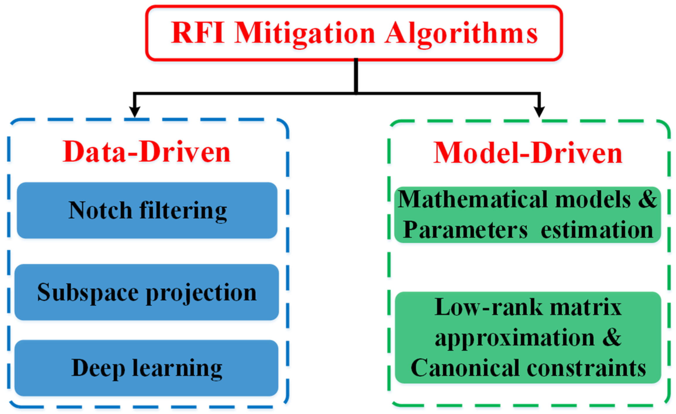
1.2. Previous Work on RFI Mitigation

RFI mitigation plays an increasingly important role in SAR systems, as it can effectively alleviate the impact of RFI on SAR image quality and improve the precision of SAR image interpretation. Furthermore, some RFI mitigation algorithms have been exploited in the SAR platforms, such as Sentinel, to promote the ability of information acquisition. Over the past few decades, there has been an intensive development of RFI mitigation algorithms, which can be summarized into two categories: data-driven algorithms and model-driven algorithms. These are depicted visually in Figure 1.

(1)

Data-Driven RFI Mitigation Algorithms

Data-driven RFI mitigation algorithms typically explore the difference between the TES and the RFI, and design a reasonable filter to eliminate the RFI in the time, frequency, or time–frequency (TF) domain. These methodologies mainly include notch filtering [14,15,16,17], subspace projection [9,10,12,18,19], and deep learning [13,20]. Notch filtering is simple and easily implemented but has a potential signal loss problem, which may reduce the quality of SAR imaging. The subspace projection strategy is performed via the statistical characteristics with less signal loss. For example, Zhou et al. utilized the energy difference between NBI and TES to form an NBI mitigation algorithm based on Eigen-subspace projection [9]. However, the performance of subspace projection algorithms may be compromised by RFI if its statistical characteristics vary greatly over time. For the RFI mitigation algorithms based on deep learning [13,20,21], the outcome is restricted by the quantity and quality of available training samples.

(2)

Model-Driven RFI Mitigation Algorithms

Unlike the data-driven algorithms, model-driven RFI mitigation algorithms generally seek to develop mathematical representations of RFI, and they apply model analysis for detecting and eliminating RFI. One typical strategy of this category utilizes multi-parameter mathematical models to characterize RFI and estimates the model parameters through the observed data to reconstruct RFI [22,23,24,25]. For example, Guo et al. made use of the statistical distribution of RFI and TES and reconstructed the RFI based on the maximum a posteriori estimation. However, the performance of these methods depends heavily on the completeness and accuracy of the mathematical model. Moreover, the process of multi-parameter estimation requires extensive computational resources.

In view of the difficulty of exact estimation in multi-parameter mathematical models, another strategy of the model-driven RFI mitigation algorithms is introduced by virtue of low-rank matrix approximation and canonical constraints. This strategy utilizes the hypothesis of the low-rank and sparse properties for different components in the SAR data [26,27,28,29,30,31,32,33,34,35], and is realized by the different ordering norms in some representation domains. It significantly reduces the difficulty and complexity of parameter estimation compared with the multi-parameter mathematical model. In light of the sparse property of RFI in the frequency domain, Nguyen et al. introduced sparse recovery algorithms to reconstruct RFI [26]. In addition, inspired by the low-rank characteristic for RFI and the sparsity property for TES, the robust principal component analysis method was exploited to separate the RFI and TES [11,29,30,31,32,33]. For example, Su et al. combined the low-rank characteristics of NBI in the TF domain with the sparse hypothesis of the TES, and achieved NBI suppression based on the go decomposition (GoDec) algorithm [11]. This strategy of model-driven RFI mitigation algorithms is based on the structural characterization of RFI and TES, and its performance heavily depends on the model’s accuracy.

1.3. Related Problems

As discussed above, the data-driven RFI mitigation algorithms may have the problems of signal loss and instability, and the deep learning strategy lacks interpretability compared to the other RFI mitigation approaches. Therefore, more attention has been paid to model-driven RFI mitigation algorithms. However, the existing model-driven RFI mitigation algorithms may suffer from the inaccuracy of the RFI reconstruction model, which only utilizes the partial characteristics of RFI and TES [29,30,31,32,33]. Additionally, they may be limited by the slow convergence speed, resulting in unsuitability for practical implementation. Thus, the objective of this study is to exploit the novel model-driven RFI mitigation algorithms to improve the accuracy of the RFI reconstruction model and accelerate the convergence speed of the alternative iteration.

1.4. Contributions

In this paper, a novel RFI detection algorithm based on TF skewness is proposed at first. It utilizes a statistical difference between the RFI-free SAR echo and the RFI-contaminated echo, namely that the RFI-free SAR echo follows a Gaussian-like distribution while the RFI-contaminated echo deviates significantly from a Gaussian distribution. Then, the RFI detection can be modeled as a binary hypothesis and achieved adaptively with the help of the Neyman–Pearson criterion. Based on the structural analysis of spectrograms, the first new model combining the low-rank and double sparse (LRDS) properties is proposed to improve the model accuracy and degrade the signal recovery error. The LRDS algorithm introduces both the low-rank and sparse property for an RFI matrix as restricted constraints in the RFI reconstruction model, under the sparse assumption for TES in the TF domain. Meanwhile, the alternative direction iteration strategy is exploited to optimize the complex multivariable reconstruction model. It can obtain a better RFI mitigation performance and converge faster due to the more accurate RFI mitigation model. However, the sparsity constrains the overall structural characteristic of the RFI matrix and needs an appropriate sparsity parameter, which is always tuned manually. Hence, the other TF constraint, the joint low-rank and sparsity (TFC-LRS) algorithm, is proposed to ameliorate this deficiency. The TF constraint concept is introduced to update the sparse representation in virtue of the aggregation property of RFI in the TF domain. As a result, there is no need to manually tune the sparsity parameter of RFI, which is replaced by the TF constraint matrix that is determined adaptively by the Neyman–Pearson criterion. Finally, the well-focused SAR image is obtained by incorporating conventional SAR imaging methods for the recovered SAR data. Meanwhile, RFI mitigation experiments on both simulated and measured datasets verify the effectiveness, superiority, and robustness of the proposed algorithms.

According to the above discussion, the main contributions of this paper can be summarized as follows:

(1)

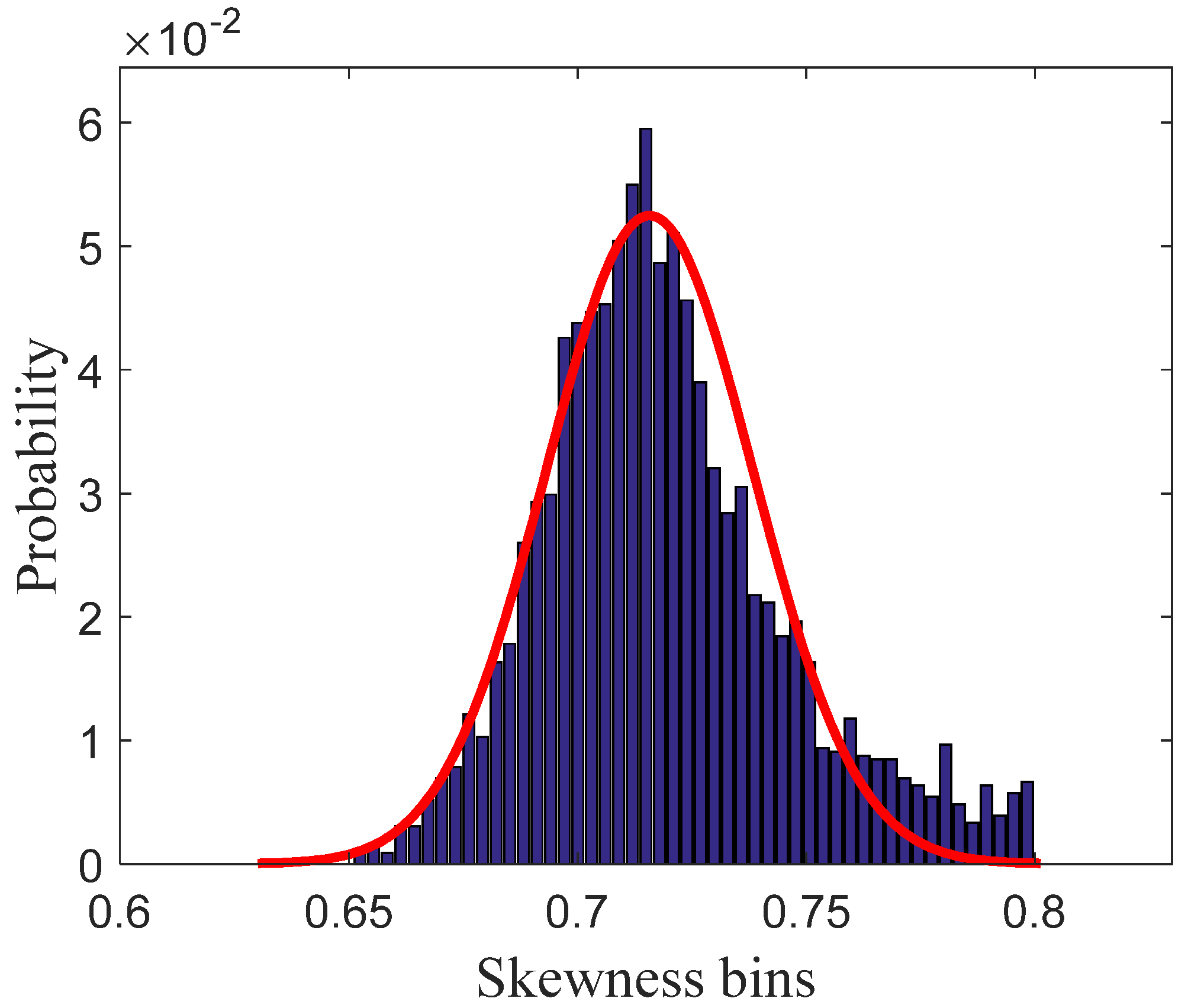
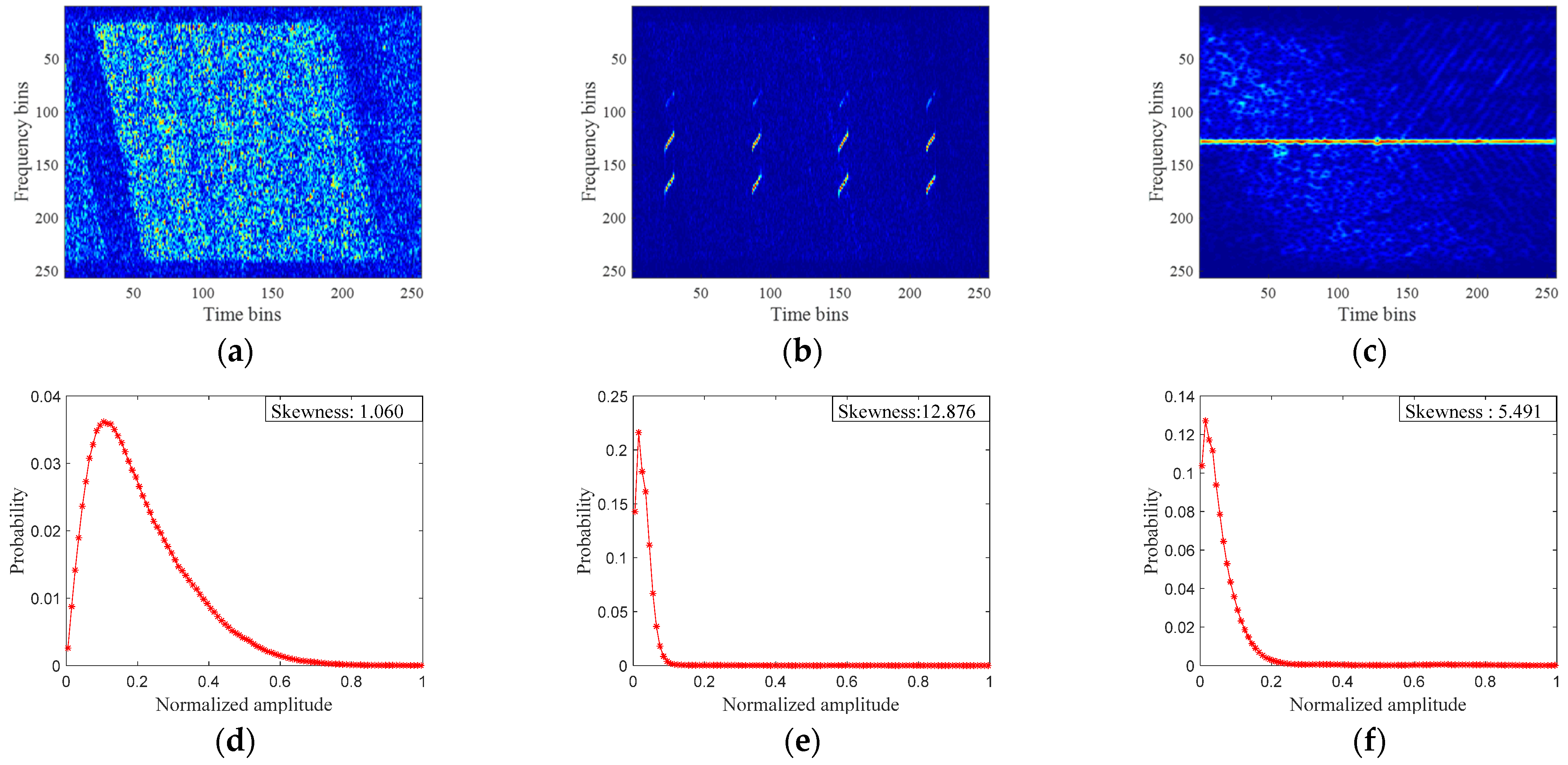
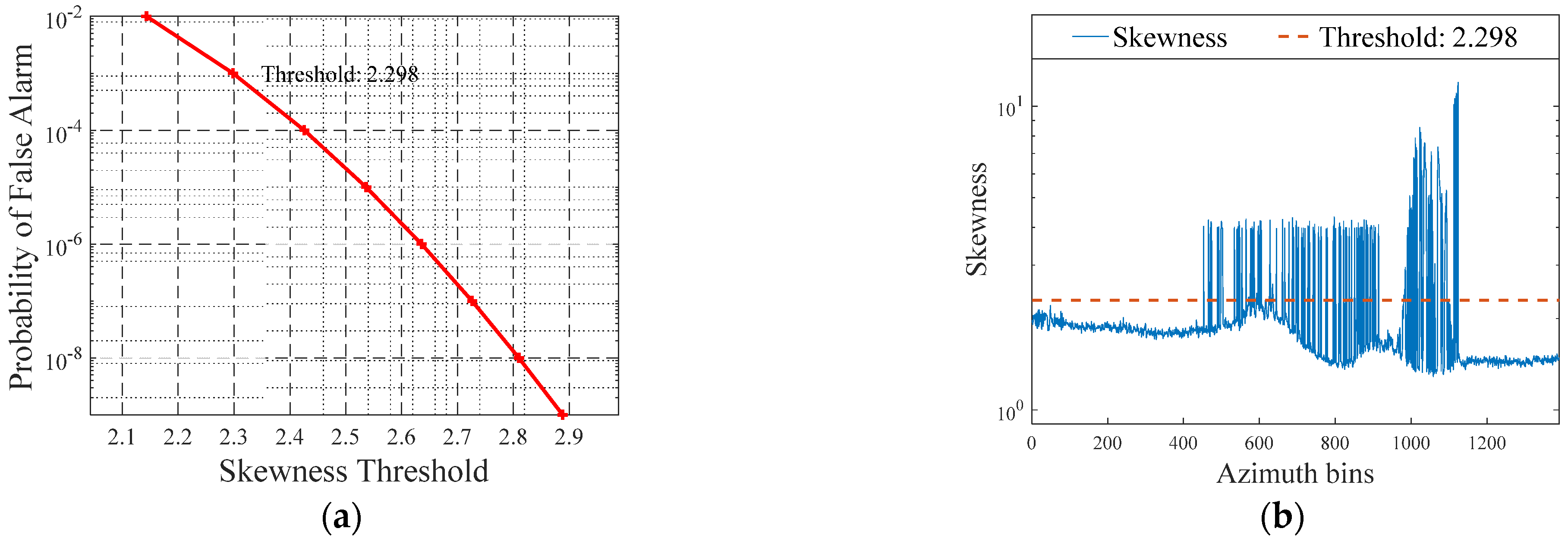
An adaptive RFI detection method based on TF skewness is proposed. Aiming to solving the poor robustness of the existing RFI detection methods, this paper introduces TF skewness to measure the non-Gaussianity of the echo in the TF domain. It also achieves adaptive statistical detection of RFI with the Neyman–Pearson criterion, which is suitable for detecting both NBI and WBI.

(2)

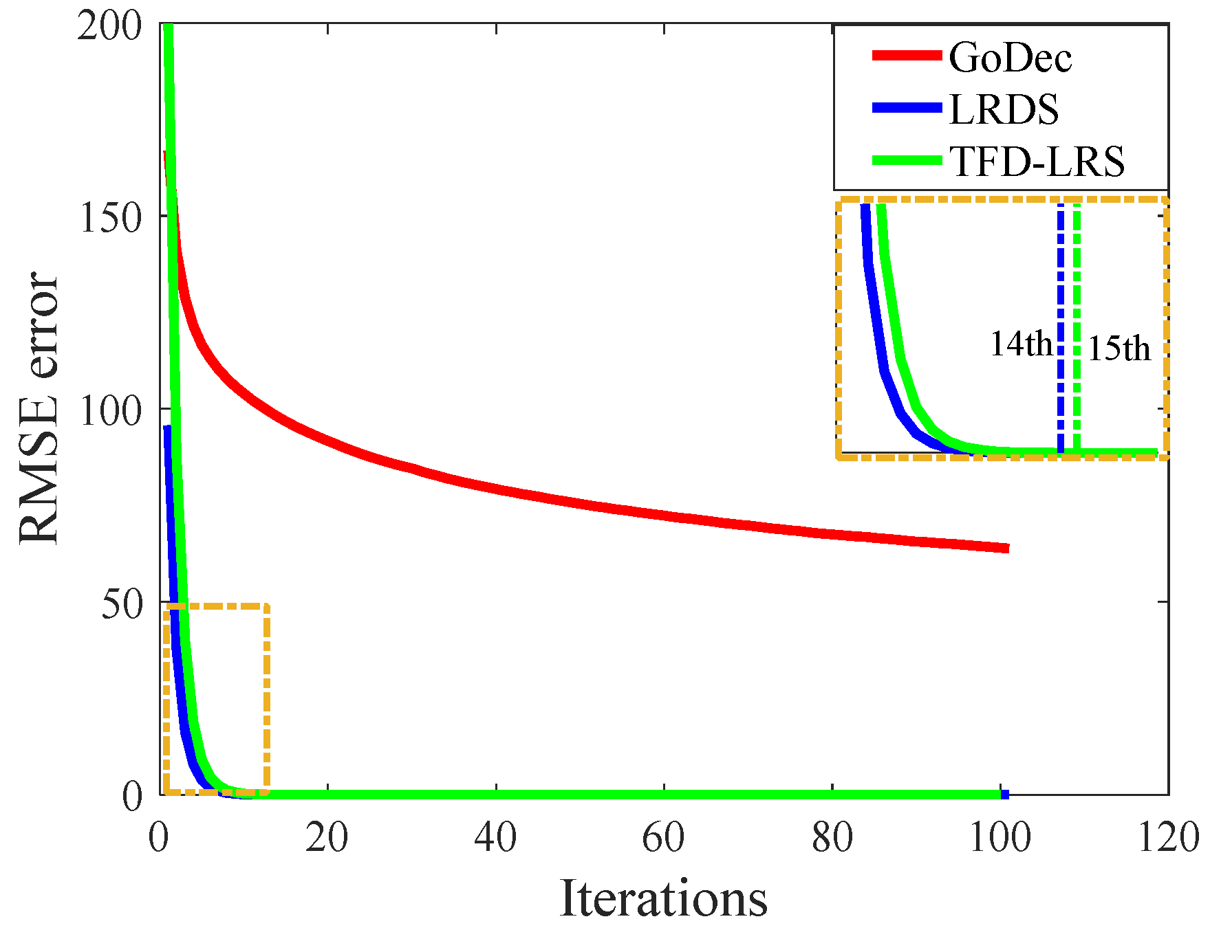
The LRDS algorithm is proposed to improve the accuracy of the RFI mitigation model and accelerate its convergence speed. Based on the TF analysis of the measured data, this paper introduces the low-rank and sparsity characteristics for RFI. Meanwhile, a more accurate RFI reconstruction model is proposed, which restrains the sparsity and low-rank property of RFI and the sparsity of TES simultaneously. The LRDS algorithm promotes the accuracy of the RFI reconstruction model with less signal recovery error and significantly reduces the iteration number to find the optimal solution.

(3)

The TFC-LRS algorithm is formulated to specify the sparsity of RFI. By virtue of the aggregation property of RFI in the TF domain, the TF constraint concept is introduced to replace the sparsity of RFI. Compared with LRDS, TFC-LRS improves the model accuracy of RFI reconstruction and reduces the signal loss further without slowing down the convergence speed.

The remainder of this paper is organized as follows. Section 2 presents the flowchart of the proposed RFI mitigation algorithms incorporating the SAR imaging procedure. In addition, it explains the statistical detection of RFI in the TF spectrograms via skewness and establishes the RFI reconstruction model based on the TF structural analysis. In Section 3, it formulates the LRDS and TFC-LRS algorithms to minimize the reconstruction error iteratively. Then, Section 4 offers the computational complexity analysis of the proposed algorithms and presents quantitative evaluation metrics. Meanwhile, RFI mitigation experiments conducted on simulated and measured SAR datasets are demonstrated in Section 5. At last, the discussion and conclusion are presented in Section 6 and Section 7, respectively.

Notations and abbreviations: Throughout this paper, the matrices are denoted by boldface capital letters, e.g., $A$, vectors are denoted by boldface lowercase letters, e.g., $a$, and scalars are denoted by the lowercase letters and the Greek characters, e.g., $a$ and $\alpha$. Additionally, there are some abbreviations to simplify the academic terminology, which are listed in

Table 1. Comparison table of abbreviations.

Abbr.	Full Name	Abbr.	Full Name
SAR	Synthetic aperture radar	TES	Target echo signal
RFI	Radio frequency interference	TF	Time–frequency
GoDec	Go decomposition	WBI	Wideband interference
LRDS	Low-rank and double sparsity	NBI	Narrowband interference
TFC-LRS	TF constraint joint low-rank and sparsity	SNR	Signal-to-noise ratio
STFT	Short-time Fourier transform	SVT	Singular value threshold
SVD	Singular value decomposition	BRP	Bilateral random projection
MDL	Minimum description length	SDR	Signal distortion ratio
SSIM	Structural similarity index measure	MNR	Multiplicative noise ratio
ISNF	Instantaneous-spectrum notch filtering	ESP	Eigenspace projection

.

2. Algorithm Model Formulation

In this section, the framework of the RFI mitigation scheme in this paper is first demonstrated. Then, the RFI statistical detection method based on TF skewness is presented and the structural properties of different components in SAR echo are analyzed. Meanwhile, the RFI reconstruction model is derived, providing theoretical foundations for the following discussions.

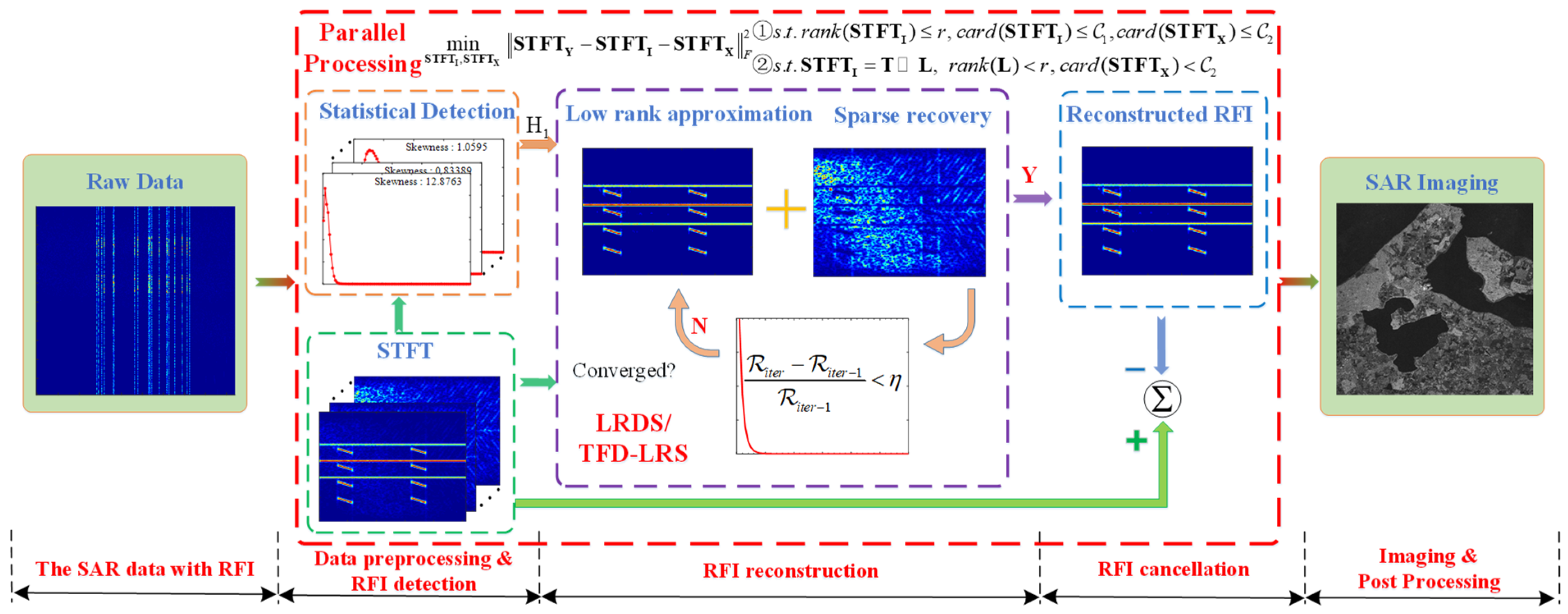
2.1. Flowchart of the Proposed Algorithms

The flowchart of the proposed algorithms is illustrated in Figure 2, which is applied in parallel for SAR data along the azimuth dimension. Firstly, the original SAR data are converted into the TF spectrograms by means of short-time Fourier transform (STFT). Furthermore, the RFI-contaminated SAR echo is detected adaptively based on a statistical difference, which is measured by TF skewness. Then, the different signal components are extracted iteratively until the RFI mitigation algorithm’s convergence from the RFI-corrupted SAR echo. Finally, the TES is recovered by interference cancellation, and the well-focused SAR image can be obtained incorporated with the state-of-the-art SAR imaging algorithm.

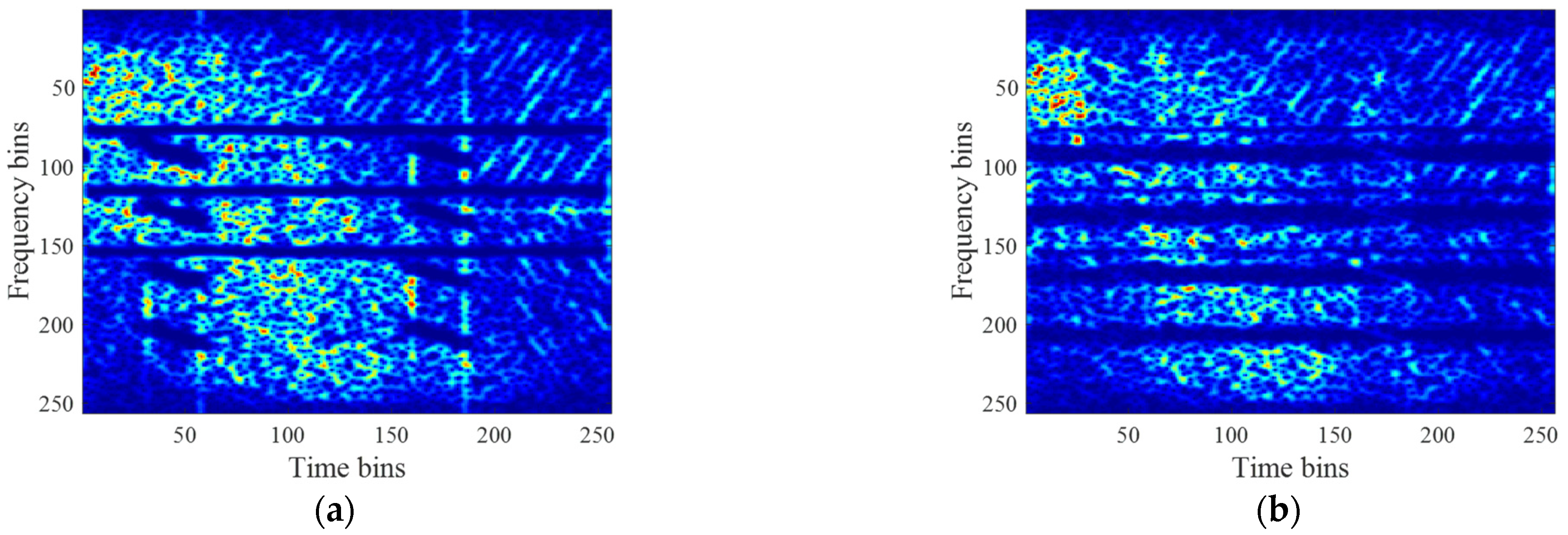
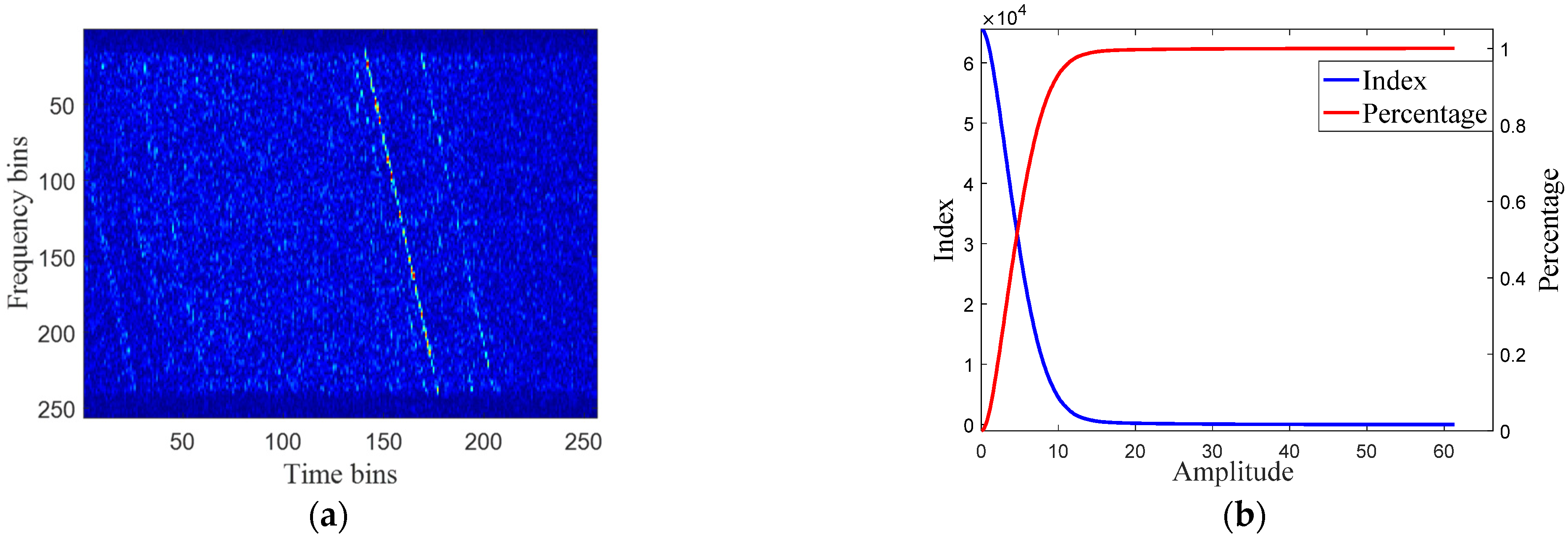
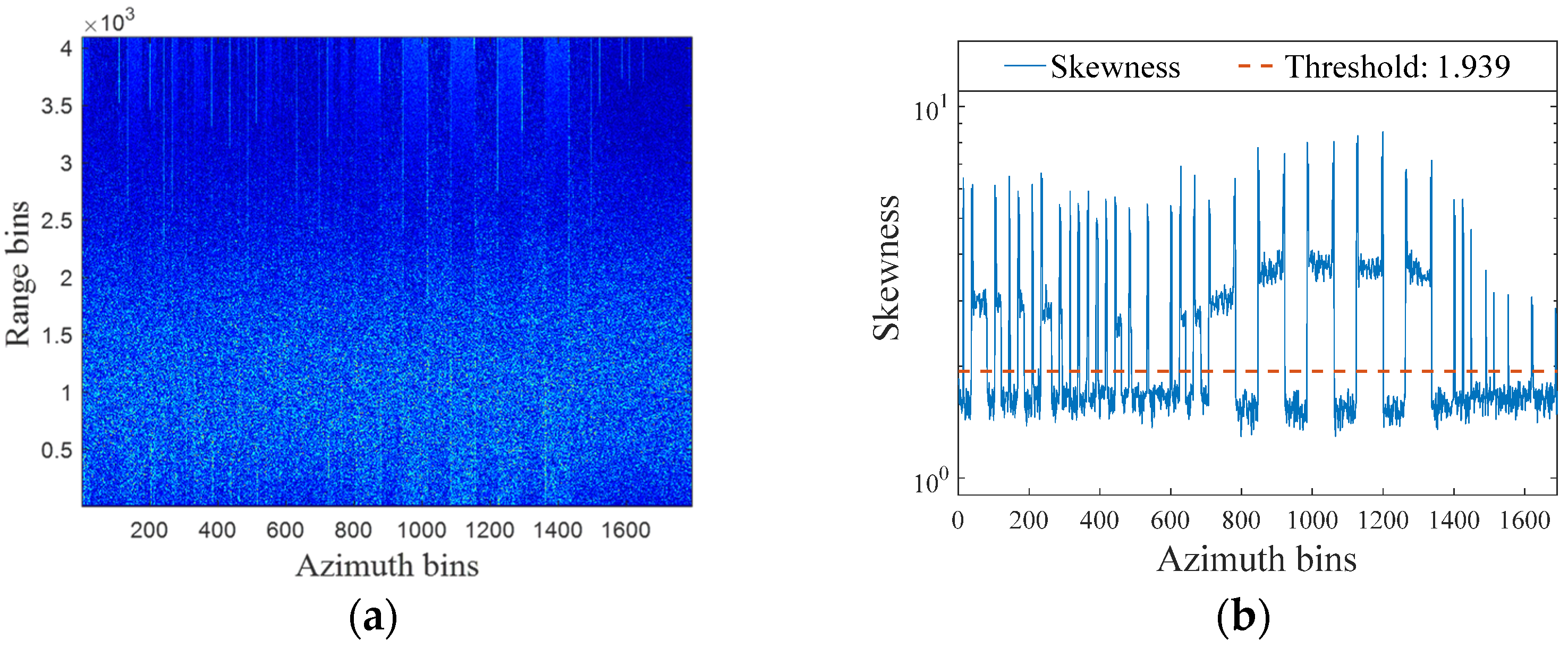
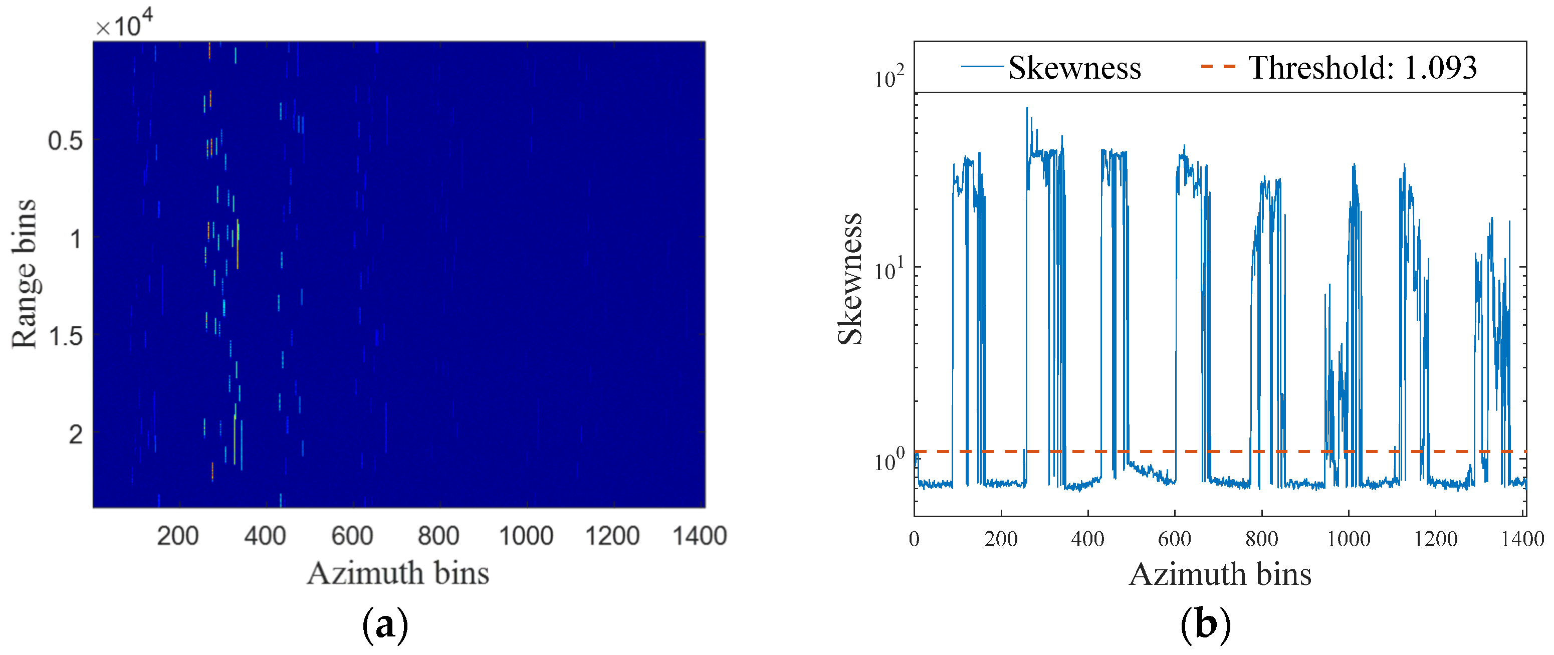
2.2. RFI Formulation and Detection

A SAR echo signal $Y\left(t,\widehat{t}\right)$ can be characterized as a mixture of the useful TES $X\left(t,\widehat{t}\right)$, RFI $I\left(t,\widehat{t}\right)$, and additive noise $N\left(t,\widehat{t}\right)$, which can be expressed as [32]

$$Y\left(t,\widehat{t}\right)=X\left(t,\widehat{t}\right)+I\left(t,\widehat{t}\right)+N\left(t,\widehat{t}\right)$$

(1)

where $\left(t,\widehat{t}\right)$ denotes the $t$th range sample of the $\widehat{t}$th snapshot, and $I\left(t,\widehat{t}\right)$ includes the NBI and WBI.

Generally, NBI is concentrated within a limited number of frequency bins, and it can be modeled as a summation of series monochromatic components with time-varying envelopes [36]. The mathematical representation can be expressed as

$$I_{NB}\left(t,\widehat{t}\right)={\displaystyle \sum _{k=1}^K{A}_k\left(t,\widehat{t}\right)\cdot }\exp \left(2\pi f_{k}t+{\varphi }_k\right)$$

(2)

where $A_k$, $f_k$ and ${\varphi }_k$ denote the complex envelope, frequency and initial phase of the $k$th jamming component, respectively. As for WBI, there are two major forms, i.e., chirp-modulated WBI and sinusoidal-modulated WBI [37,38]. The chirp-modulated WBI is characterized as

$$I_{CM}\left(t,\widehat{t}\right)={\displaystyle \sum _{k=1}^K{A}_k\left(t,\widehat{t}\right)\exp \left\{j\left(2\pi f_{k}t+\pi {\gamma }_k{t}^2\right)\right\}}$$

(3)

where $A_k$, $f_k$ and ${\gamma }_k$ are the amplitude, frequency and chirp rate of the $k$th component. Moreover, the sinusoidal-modulated WBI can be expressed as

$$I_{SM}\left(t,\widehat{t}\right)={\displaystyle \sum _{k=1}^K{A}_k\left(t,\widehat{t}\right)\exp \left\{j{\beta }_k\sin \left(2\pi f_{k}t+{\varphi }_k\right)\right\}}$$

(4)

where $A_k$, ${\beta }_k$, $f_k$, and ${\varphi }_k$ are the amplitude, modulation factor, frequency, and initial phase of the $k$th component. In measured data, the WBI signatures can always be considered as the combination of these two special forms.

Due to the large synthetic aperture time of SAR and the time-varying property of interference, RFI may not be present in all snapshots. Therefore, it is of great significance to identify whether RFI exists in a single echo, avoiding the unnecessary signal loss and extra cost of the computational resources. However, the existing RFI detection methods are mainly appropriate for the simple and isolated NBI, and may fail in the increasingly complex electromagnetic environment. Therefore, this paper develops an RFI detection method that is robust for both NBI and WBI.

The essence of RFI detection is to extract and quantify the maximum characteristic difference between RFI and TES. It must be able to analyze the universal feature of NBI and WBI, meaning that considering only the time or frequency domain will be insufficient. Therefore, the STFT is utilized to combine the time and spectra features of SAR echo in the two-dimensional TF domain.

Figure 3a–c show the TF spectrograms of RFI-free and RFI-contaminated SAR echoes, respectively. It is clear that there are bright areas in Figure 3b,c corresponding to RFI with stronger amplitude. Further, the statistical analyses presented in Figure 3d–f show that the statistical fitting curve without RFI is gentler, whereas it has a sharper peak and longer tail with RFI. Generally, under the complex Gaussian distribution assumption of RFI-free SAR echo, the real and imaginary parts of its TF spectrogram obey the Gaussian distribution. Therefore, the spectrogram amplitude obeys the Rayleigh distribution, which is Gaussian-like. Owing to the presence of RFI, the histograms deviate from the Gaussian distribution and concentrate in the low amplitude region, leading to a sharp left peak and a fatter right tail. Therefore, there is the theoretical condition that this non-Gaussianity can be utilized to perform RFI detection.

In the non-stationary signal field, the skewness defined as the third-order moment is one of the simplest statistical metrics to measure the deviation from a Gaussian distribution [39]. The skewness $S$ of the SAR echo spectrogram $STF{T}_Y\in {ℂ}^{M\times N}$ can be expressed as

$$S=E\left\{{\left(\frac{\left(\Vert STF{T}_Y\Vert -\mu \right)}{\sigma }\right)}^3\right\}=\frac{\frac{1}{MN}{\displaystyle \sum _m^M{\displaystyle \sum _n^N{\left(\Vert STF{T}_{Y_{mn}}\Vert -\mu \right)}^3}}}{{\left(\frac{1}{MN}{\displaystyle \sum _m^M{\displaystyle \sum _n^N{\left(\Vert STF{T}_{Y_{mn}}\Vert -\mu \right)}^2}}\right)}^{3/2}}$$

(5)

where $E\left\{\cdot \right\}$ denotes the expectation operator, $\mu$ and ${\sigma }^2$ represent the mean and variance of $STF{T}_Y$, and the term with subscript ${(\cdot )}_{mn}$ is a matrix element in the $m$th row and $n$th column. The skewness value ranges among $\left(-\infty ,+\infty \right)$. It is straightforward to show that the skewness of a pure Gaussian distribution is zero, but it deviates from zero when non-Gaussian signal sources are presented, as shown in Figure 3. A distribution with positive skewness would have a more acute peak on the left and a fatter tail on the right than the Gaussian distribution, whereas a distribution with negative skewness would have a peak on the right and a tail on the left. The stronger amplitude of RFI components indicates a positive skewness for the distribution of RFI-corrupted SAR echo. The skewness value of the RFI-free snapshot shown in Figure 3d is 1.06, whereas the RFI-corrupted pulses shown in Figure 3e,f are equal to 12.867 and 5.491, respectively. This supports the conclusion that there is an apparent statistical difference between the RFI and TES.

Therefore, the RFI detection is transformed into the skewness value judgement in the TF domain, which is a binary classification problem. The key issue in solving this problem is to determine an appropriate detection threshold, $\xi$, which is of great significance for the missing detection and the false alarm in RFI detection. It is demonstrated as follows:

$$\{\begin{array}{cc}\mathcal{S}<\xi ,\hfill & \Rightarrow {\mathrm{H}}_0:Without RFI\hfill \\ \mathcal{S}\ge \xi ,\hfill & \Rightarrow {\mathrm{H}}_1:With RFI\hfill \end{array}$$

(6)

The threshold value is critical to the accuracy of RFI detection. Hence, a comprehensive consideration of RFI missing detection and false alarm is required to obtain the best detection performance, ensuring that the false alarm rate satisfies the tolerance range. Thus, the Neyman–Pearson criterion is exploited to adaptively select the optimal threshold $\xi$, which can be expressed as [40]

$$\begin{array}{ccc}\xi =\arg \max P_D\hfill & s.t.& \hfill P_F\le \alpha \end{array}$$

(7)

where $P_D$, $P_F$ and $\alpha$ denote the probability of detection, the false alarm rate and the expected false alarm level. $P_F$ is no greater than ${10}^{-3}$, and is usually set within the range $\left[{10}^{-3},{10}^{-8}\right]$. According to the constraint of false alarm, $\alpha$ can be calculated as

$$\alpha =P_F={\displaystyle {\int }_{\xi }^{\infty }{p}_{\mathcal{S}|{\mathrm{H}}_0}\left(v\right)dv}$$

(8)

where $p_{\mathcal{S}|{\mathrm{H}}_0}\left(v\right)$ is the statistical distribution of skewness without RFI.

To analyze the mathematical representation of $p_{\mathcal{S}|{\mathrm{H}}_0}\left(v\right)$, the no-RFI SAR dataset was established first to fit the statistical distribution. This dataset was recorded by the Sentinel-1 satellite on 3 June 2021, and was not disturbed by RFI. Figure 4 shows the histograms and statistical fitting curve of skewness calculated from the no-RFI SAR dataset, which declares that the skewness $\mathcal{S}$ tends to a Gaussian distribution asymptotically. Therefore, the optimal threshold of skewness based on the Neyman–Pearson criterion is

$$\xi ={\mu }_{\mathcal{S}}+\sqrt{2{\sigma }_{\mathcal{S}}^2}{\mathrm{erf}}^{-1}\left(1-2\alpha \right)$$

(9)

where ${\mu }_{\mathcal{S}}$ and ${\sigma }_{\mathcal{S}}$ are the mean and variance of skewness, and ${\mathrm{erf}}^{-1}$ is the inverse error function. According to (6) and (9), the accurate detection of RFI-contaminated pulses in SAR data can be achieved. The representation of a single snapshot corrupted with RFI can be simplified as

$$y\left(t\right)=x\left(t\right)+i\left(t\right)+n\left(t\right)$$

(10)

2.3. The RFI Reconstruction Model

The linear reversibility of the STFT ensures that this transformation does not affect the linear superposition characteristics of the SAR echo [41]. Therefore, according to (10), the TF matrix of the SAR echo can be expressed as

$$STF{T}_Y=STF{T}_X+STF{T}_I+STF{T}_N$$

(11)

Our goal is to reconstruct the RFI and TES from the observed echo in the TF domain, and the noise can be treated as the reconstruction error based on the error modeling theory

$$\underset{STF{T}_I,STF{T}_X }{\min }f\left(STF{T}_Y,STF{T}_I,STF{T}_X\right)$$

(12)

Generally, there is an assumption of complex Gaussian distribution for the noise component in an SAR echo, and the optimization function in (12) is specified with the Frobenius norm,

$$\underset{STF{T}_I,STF{T}_X }{\min }{\Vert STF{T}_Y-STF{T}_I-STF{T}_X\Vert }_F^2$$

(13)

where ${\Vert ·\Vert }_F^2$ is the symbol of the Frobenius norm.

The error reconstruction model in (13) is under the assumption of Gaussian noise. However, it lacks the feature descriptions of RFI and TES, and is an incomplete RFI reconstruction model. To refine the model, the characteristic constraints of RFI and TES should be added based on the TF analysis.

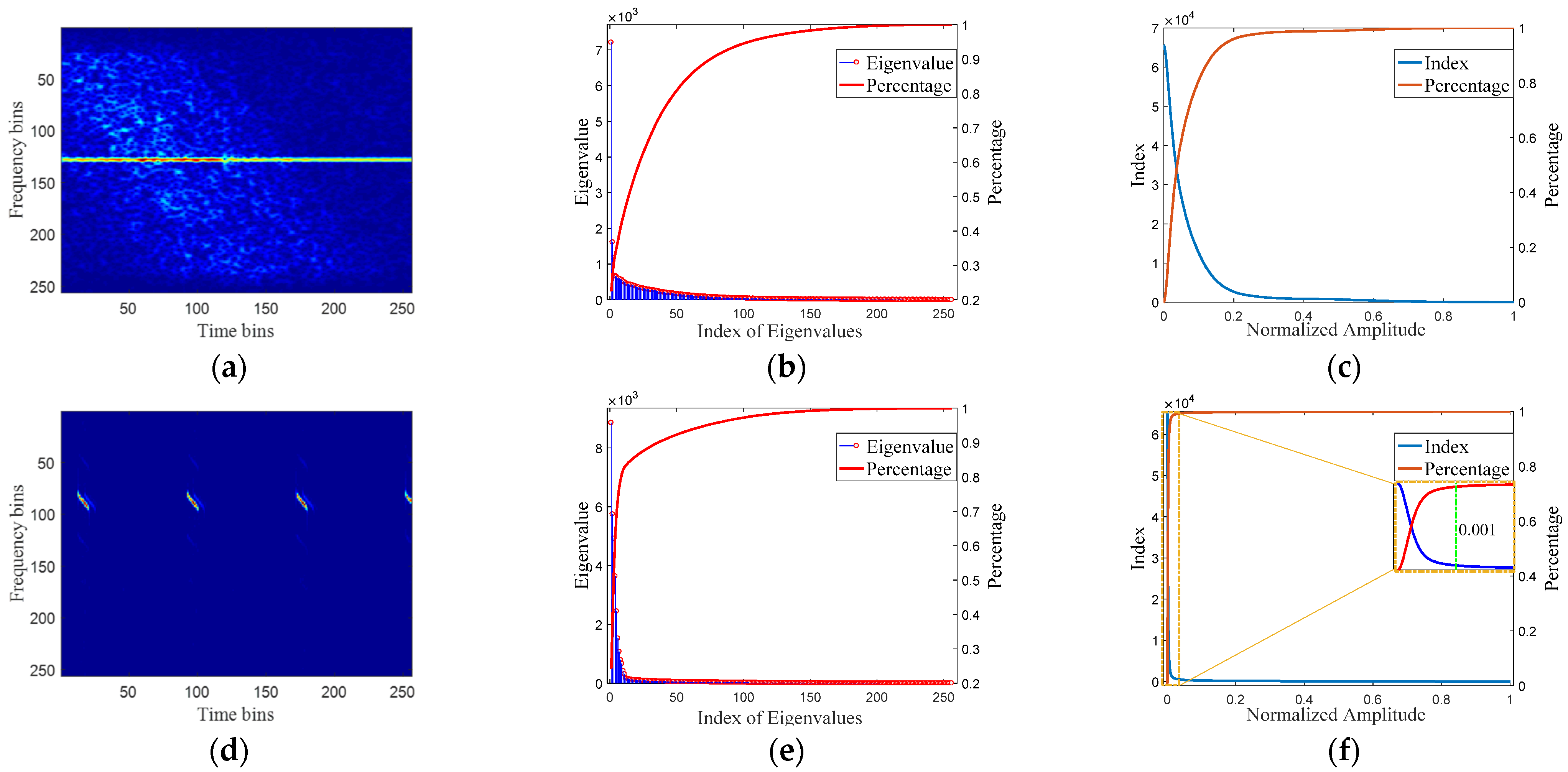
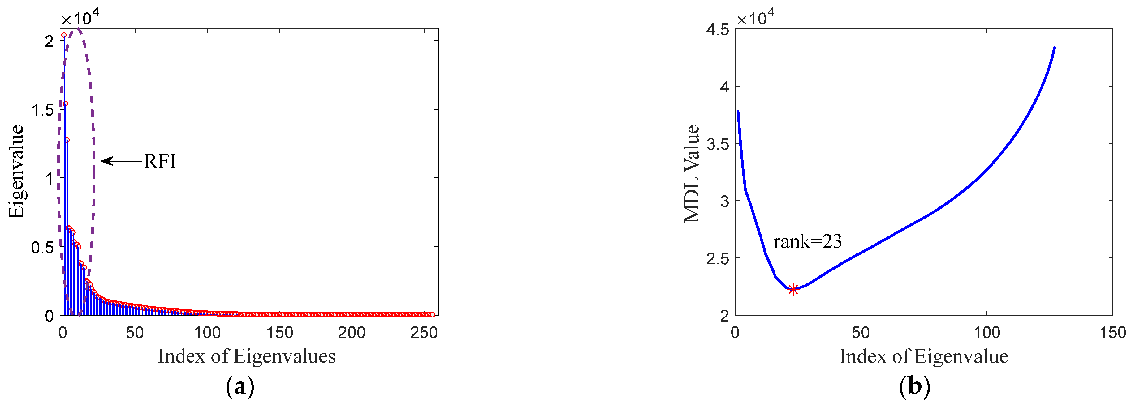
2.3.1. The Low-Rank and Sparsity Properties of RFI

There are two TF spectrograms of measured SAR echoes contaminated with NBI (Figure 5a) and WBI (Figure 5d). The bright areas in these spectrograms correspond to the RFI and only occupy a small proportion of the TF bins. This clearly indicates that RFI should possess a low-rank and sparse characteristic in the TF spectrogram. To further verify the low-rank structural feature, eigenvalue decomposition was performed on Figure 5a,d, and the corresponding results are shown in Figure 5b,e, respectively. The eigenvalues reflect the energies of different components in the SAR echo, as well as the structural redundancy of the matrix. The figures show that very few large eigenvalues are related with RFI in the spectrograms, which further demonstrates the low-rank characteristic of RFI. Meanwhile, amplitude analysis was applied to Figure 5a,d, and the results are presented in Figure 5c,f. Clearly, the number of TF bins with larger amplitudes corresponding to RFI is much lower than the total number of TF units. Figure 5c,f declare that the RFI component in the TF domain exhibits the sparse property.

Therefore, the RFI component in the TF domain can be considered as a low-rank and sparse matrix, and the constraints of RFI can be tuned in the RFI reconstruction model

$$\begin{array}{l}\underset{STF{T}_I,STF{T}_X }{\min }{\Vert STF{T}_Y-STF{T}_I-STF{T}_X\Vert }_F^2\\ s.t.rank(STF{T}_I)<r,card(STF{T}_I)<{\mathcal{C}}_1\end{array}$$

(14)

where $rank(\cdot )$ and $card(\cdot )$ denote the operators used for calculating rank and cardinality, and $r$ and ${\mathcal{C}}_1$ are the rank and sparsity of $STF{T}_I$.

2.3.2. The Sparsity of TES

As discussed above, the RFI reconstruction model, (13), was tuned with the constraint of RFI in (14). To pursue a more accurate RFI reconstruction model, the property of TES should be restricted in (14) based on TF analysis. Although the TES is noise-like compared with the strong RFI, its amplitude is stronger than the noise. Figure 6a presents the amplitude analysis result of SAR echo without RFI, and it shows that the TES only occupies several TF units, whereas noise is present throughout the TF spectrogram. Meanwhile, the percentage of TES units is less than 20% in Figure 6b, which further supports the sparsity of TES in the TF spectrogram.

Because the spectrogram of TES is a sparse matrix, the RFI reconstruction model can be optimized as

$$\begin{array}{l}\underset{STF{T}_I,STF{T}_X }{\min }{\Vert STF{T}_Y-STF{T}_I-STF{T}_X\Vert }_F^2\\ s.t.rank(STF{T}_I)\le r,card(STF{T}_I)\le {\mathcal{C}}_1\\ card(STF{T}_X)\le {\mathcal{C}}_2\end{array}$$

(15)

where ${\mathcal{C}}_2$ is the sparsity of TES.

So far, the more accurate RFI reconstruction model has been established, and the solution will be discussed in the following section.

3. Theory and Methodology

In this section, two iterative optimization algorithms are proposed to solve the RFI reconstruction model based on the low-rank and sparse property of the components in the SAR echo. The first algorithm utilizes the LRDS property to reconstruct RFI. It works well for RFI mitigation but with a few unnecessary signal losses. Moreover, the TFC-LRS algorithm introduces the concept of TF constraint instead of sparsity for RFI, and establishes a more accurate RFI reconstruction model.

3.1. LRDS Algorithm

The RFI reconstruction model in (15) is a multivariate optimization problem under several constraints, which is difficult to solve directly due to the coupled characteristics. Naturally, the alternative iteration strategy is exploited to optimize the model parameters. As for the reconstruction model in (15), it can be divided into three sub-problems according to the constraints: the low-rank matrix approximation and the sparse reconstruction for RFI and TES. Thereby, the multivariate optimization problem is iteratively transformed into global optimizations for sub-problems. The sub-problems can be expressed as

$$\begin{array}{l}{L}^{\left(l+1\right)}=\arg \underset{L}{\min }{\Vert STF{T}_Y-L^{(l)}-STF{T}_X^{(l)}\Vert }_F^2\\ s.t. \mathrm{rank} \left(L^{(l)}\right)\le r\end{array}$$

(16a)

$$\begin{array}{l}STF{T}_I^{(l+1)}=\arg \underset{STF{T}_I}{\min }{\Vert L^{\left(l+1\right)}-STF{T}_I^{(l)}\Vert }_F^2\\ s.t. card\left(STF{T}_I^{(l)}\right)\le {\mathcal{C}}_1\end{array}$$

(16b)

$$\begin{array}{l}STF{T}_X^{(l+1)}=\arg \underset{STF{T}_S}{\min }{\Vert STF{T}_Y-STF{T}_I^{(l+1)}-STF{T}_X^{(l)}\Vert }_F^2\\ s.t. card\left(STF{T}_X^{(l)}\right)\le {\mathcal{C}}_2 \end{array}$$

(16c)

where $L$ is the auxiliary variable representing the result of low-rank approximation, and the superscript ${(·)}^l$ denotes the $l$th iteration.

The low-rank approximation sub-problem in (16a) can be solved by the singular value threshold (SVT) algorithm, which utilizes the selection of larger singular values to perform low-rank approximation based on the relationship between rank and singular value. It can be characterized mathematically as

$$L_I^{(l+1)}=SVT\left(STF{T}_Y-STF{T}_X^{(l)}\right)=U{\mathcal{P}}_{{\mathcal{H}}_0}(\Lambda )V$$

(17)

where $U$, $\Lambda$, and $V$ correspond to the left projection matrix, singular value matrix and right projection matrix, respectively, and $STF{T}_Y-STF{T}_X^{(l)}=U\Lambda V$. Meanwhile, ${\mathcal{H}}_0:\left|{\Lambda }_{mn\in {\mathcal{H}}_0}\right|\ge \left|{\Lambda }_{mn\in {\overline{\mathcal{H}}}_0}\right|,\left|{\mathcal{H}}_0\right|\le r$, and ${\mathcal{P}}_{{\mathcal{H}}_0}(\Lambda )$ denotes the hard threshold mapping for extraction of the first larger singular values.

However, there is a high computation burden for singular value decomposition (SVD), which is the main step of SVT and requires $\min \left(M{N}^2,M^{2}N\right)$ flops per iteration. It is impractical to implement SVD when the scale of the processing matrix is too large. However, a large scale TF matrix is typically generated to ensure the time and frequency resolution.

In order to reduce the computational burden and accelerate the iteration convergence, the bilateral random projection algorithm (BRP) is introduced to replace the SVT to extract the low-rank component. First, the left random projection matrix $B_2\in {ℂ}^{M\times r}$ and the right random projection matrix $B_1\in {ℂ}^{N\times r}$ for the dense matrix $Z^{(l)}=STF{T}_Y-STF{T}_X^{(l)}\in {ℂ}^{M\times N}$ are defined with the rank $r$. By utilizing the auxiliary variables $D_1=Z^{(l)}{B}_1$ and $D_2={\left(Z^{(l)}\right)}^H{B}_2$, the fast rank-$r$ approximation of $Z^{(l)}$ is

$$L^{\left(l+1\right)}=D_1{\left(B_2^H{D}_1\right)}^{-1}{D}_2^H$$

(18)

To prevent the slow decay of the singular values, a power scheme is introduced to improve the efficiency of BRP, which is performed for the matrix $\tilde{Z}={\left(Z^{(l)}{Z}^{(l)}{}^{{}^H}\right)}^q{Z}^{(l)}$ instead of $Z^{(l)}$. Based on BRP, the fast rank-$r$ approximation of $\tilde{Z}$ is

$$\tilde{L}=D_1{\left(B_2^H{D}_1\right)}^{-1}{D}_2^H$$

(19)

where $B_2=D_1=\tilde{L}{B}_1$ and $B_1=D_2={\tilde{L}}^H{B}_2$ are utilized to update the random projection matrix. In order to obtain the rank $r$ approximation of $Z^{(l)}$, the QR decomposition is calculated as $D_1=Q_1{R}_1,D_2=Q_2{R}_2$. Thus, the fast rank-$r$ approximation of $Z^{(l)}$ is

$$L^{\left(l+1\right)}={\left(\tilde{L}\right)}^{\frac{1}{2q+1}}=Q_1{\left[R_1{\left(B_2^H{D}_1\right)}^{-1}{R}_2^H\right]}^{\frac{1}{2q+1}}{Q}_2^H$$

(20)

As for the sparse reconstruction sub-problem, the hard threshold mapping is also utilized to update the TES in traditional methods, which can be characterized as

$$STF{T}_X^{(l+1)}={\mathcal{P}}_{{\mathcal{H}}_1}\left(STF{T}_Y-STF{T}_I^{(l)}\right)$$

(21)

where ${\mathcal{H}}_1:\left|{\left(STF{T}_Y-STF{T}_I^{(l)}\right)}_{mn\in {\mathcal{H}}_1}\right|\ge \left|{\left(STF{T}_Y-STF{T}_I^{(l)}\right)}_{mn\in {\overline{\mathcal{H}}}_1}\right|,\left|{\overline{\mathcal{H}}}_1\right|\le {\mathcal{C}}_2$, and ${\mathcal{P}}_{{\mathcal{H}}_1}(\cdot )$ denotes the mapping function to reserve the ${\mathcal{C}}_2$ largest values. However, for complex matrices, the hard threshold mapping method would cause some reconstruction errors and make the algorithm converge slowly. Therefore, the soft threshold mapping method is introduced to solve sparse reconstruction sub-problems in this paper.

As for the sparse reconstruction of RFI in (16b), the solution of applying the revised soft threshold mapping is

$$STF{T}_I^{(l+1)}={\mathcal{P}}_{{\Omega }_1}\left(L^{\left(l+1\right)}\right)$$

(22)

where ${\mathcal{P}}_{{\Omega }_1}(·)$ denotes the entry-wise soft threshold mapping, specifically expressed as

$${\mathcal{P}}_{{\Omega }_1}\left(E_{mn}\right)={\mathcal{P}}_{H_1}\left(E_{mn}\right)-\mathrm{sign}\left(E_{mn}\right)\cdot {\left|sort\left(E\right)\right|}_{{\mathcal{C}}_1+1}$$

(23)

Here, ${\mathcal{P}}_H(·)$ denotes the hard threshold mapping of matrix elements, $\mathrm{sign}\left(a\right)=a/\left|a\right|$, ${\left|sort(·)\right|}_{{\mathcal{C}}_1+1}$ extracts the $\left({\mathcal{C}}_1+1\right)$th largest value in descending order, and $E$ denotes an arbitrary matrix.

Similarly, the sparse recovery of TES is expressed as

$$STF{T}_X^{(l+1)}={\mathcal{P}}_{{\Omega }_2}\left(STF{T}_Y-STF{T}_I^{(l+1)}\right)$$

(24)

where ${\mathcal{P}}_{{\Omega }_2}\left(E_{mn}\right)={\mathcal{P}}_{{\mathcal{H}}_2}\left(E_{mn}\right)-\mathrm{sign}\left(E_{mn}\right)\cdot {\left|sort\left(E\right)\right|}_{{\mathcal{C}}_2+1}$.

Therefore, the optimization problem of (16) can be solved iteratively by (20), (22), and (24). It can provide an accurate reconstruction result of RFI and TES until convergence. The LRDS algorithm is summarized in Algorithm 1, and the detailed performance will be presented in the following subsection.

Algorithm 1. The Proposed LRDS Algorithm

Input: $STF{T}_Y$, $r$, ${\mathcal{C}}_1$, ${\mathcal{C}}_2$, $q$

Initialization: $L^{\left(0\right)}$, $STF{T}_I^{(0)}$, $STF{T}_X^{(0)}$, $l=0$

While ${\Vert STF{T}_Y-STF{T}_I^l-STF{T}_X^l\Vert }_F^2/{\Vert STF{T}_Y\Vert }_F^2>\eta$ do

Low rank approximation: $L^{\left(l+1\right)}=Q_1{\left[R_1{\left(A_2^H{Y}_1\right)}^{-1}{R}_2^H\right]}^{1/\left(2q+1\right)}{Q}_2^H$;

RFI reconstruction: $STF{T}_I^{(l+1)}={\mathcal{P}}_{{\Omega }_1}\left(L^{\left(l+1\right)}\right)$;

TES recovery: $STF{T}_X^{(l+1)}={\mathcal{P}}_{{\Omega }_2}\left(STF{T}_Y-STF{T}_I^{(l+1)}\right)$;

$l=l+1$

End while.

Output: $STF{T}_I=STF{T}_I^{(l)}$, $STF{T}_X=STF{T}_X^{(l)}$

3.2. TFC-LRS Algorithm

The TF sparsity of RFI describes the structural property in the whole TF spectrogram, and LRDS establishes a more accurate RFI reconstruction model combined with the low-rank and sparse properties. However, the particularity of the RFI structural distribution makes it possible to improve the accuracy of the RFI reconstruction model further. As shown in Figure 5, the RFI is aggregated in the TF spectrogram due to the continuous modulation in the time and frequency domains, resulting in a special sparse structure. Therefore, the TF constraint concept is introduced to restrict the location of RFI during the alternative iteration.

Inspired by the adaptive statistical detection of RFI based on TF skewness, the TF constraint matrix can be obtained through a binary detection, and the optimal threshold $\lambda$ is calculated as

$$\lambda =\arg \max {P^{\prime }}_D\begin{array}{cc}s.t.& {P^{\prime }}_F\le {\alpha }^{\prime }\end{array}$$

(25)

where ${P^{\prime }}_D$ and ${P^{\prime }}_F$ are the probability of detection and false alarm, and ${\alpha }^{\prime }={P^{\prime }}_F={\displaystyle {\int }_{\lambda }^{\infty }{p}_y\left(v\right)dv}$ is the maximum false alarm probability level. As discussed above, the probability distribution function $p_y\left(v\right)$ is the Rayleigh distribution for the amplitude in the TF matrix without RFI. Therefore, the optimal threshold is

$$\lambda =S_{Ray}^{-1}\left({\alpha }^{\prime }\right)=\sqrt{-{\delta }_y\ln \left({\alpha }^{\prime }\right)}$$

(26)

where $S_{Ray}^{-1}(·)$ is the inverse survivor function of the Rayleigh distribution and ${\delta }_y$ is the parameter of $p_y\left(v\right)$. According to (26), the TF constraint matrix can be obtained easily, as follows:

$$T_{mn}=\max \left\{\mathrm{sign}\left(\left|STF{T}_{Y_{mn}}\right|-\lambda \right),0\right\}$$

(27)

Based on the TF constraint matrix $T$, the reconstruction model can be updated as

$$\begin{array}{l}\underset{STF{T}_I,STF{T}_X }{\min }{\Vert STF{T}_Y-STF{T}_I-STF{T}_X\Vert }_F^2\\ s.t.STF{T}_I=T\odot L,rank(L)<r\\ card(STF{T}_X)<{\mathcal{C}}_2\end{array}$$

(28)

where $L$ is the low-rank approximation of RFI. Specifically, the optimization problem shown in (28) can be decomposed into two sub-problems, namely RFI reconstruction and TES recovery, which are updated alternatively:

$$\begin{array}{l}STF{T}_I^{(l+1)}=\arg \underset{STF{T}_I}{\min }{\Vert STF{T}_Y-STF{T}_I^{(l)}-STF{T}_X^{(l)}\Vert }_F^2\\ \hfill s.t.STF{T}_I^{(t)}=T\odot L^{\left(l\right)},rank(L^{\left(l\right)})<r\end{array}$$

(29a)

$$\begin{array}{l}STF{T}_X^{(l+1)}=\arg \underset{STF{T}_X}{\min }{\Vert STF{T}_Y-STF{T}_I^{(l+1)}-STF{T}_X^{(l)}\Vert }_F^2\\ \hfill s.t.card(STF{T}_X)<{\mathcal{C}}_2\hfill \end{array}$$

(29b)

Referring to (20), the solution of the RFI reconstruction sub-problem in (29a) is

$$STF{T}_I^{(l+1)}=T\odot \left\{Q_1{\left[R_1{\left(B_2^H{D}_1\right)}^{-1}{R}_2^H\right]}^{1/\left(2q+1\right)}{Q}_2^H\right\}$$

(30)

Referring to (24), the solution of the TES sparse recovery sub-problem in (29b) is

$$\begin{array}{c}STF{T}_X^{(l+1)}=P_{H_2}\left[{\left(STF{T}_{N^{\prime }}\right)}_{mn}\right]-\mathrm{sign}\left[{\left(STF{T}_{N^{\prime }}\right)}_{mn}\right]\cdot {\left|sort\left(STF{T}_{N^{\prime }}\right)\right|}_{{\mathcal{C}}_2+1}\\ STF{T}_{N^{\prime }}=STF{T}_Y-STF{T}_I^{(l+1)}\end{array}$$

(31)

The reconstruction model, (29), can be solved by iteratively optimizing (30) and (31). At last, the TFC-LRS algorithm is summarized in Algorithm 2, and a detailed analysis will be presented in the following subsection.

3.3. Analysis of the Prior Parameters

The proposed LRDS and TFC-LRS algorithms iteratively optimize the RFI reconstruction model, joining the sparsity and low-rank properties while extracting the RFI and TES alternatively. Meanwhile, the well-focused SAR image will be obtained from the recovered TES via the state-of-the-art SAR imaging algorithm. However, there would be some unavoidable errors for different components’ reconstruction. Therefore, the RFI cancellation strategy is introduced to reduce the system error, and it is expressed as follows:

$$\hat{x}\left(t\right)=ISTFT\left[STF{T}_Y-STF{T_I}^{\ast }\right]$$

(32)

where $ISTFT(·)$ denotes the inverse short-time Fourier transform, and $STF{T_I}^{\ast }$ denotes the reconstructed RFI matrix until iteration convergence. At last, the complete RFI mitigation procedure is presented, and the RFI-free data can be obtained in parallel with the detection algorithm proposed in this paper.

Algorithm 2. The Proposed TFC-LRS Algorithm

Input: $STF{T}_Y$, $r$, ${\mathcal{C}}_2$, $q$

Initialization: $STF{T}_I^{(0)}$, $STF{T}_X^{(0)}$, $T$, $l=0$

While ${\Vert STF{T}_Y-STF{T}_I^l-STF{T}_X^l\Vert }_F^2/{\Vert STF{T}_Y\Vert }_F^2>\eta$ do

RFI reconstruction: $STF{T}_I^{(l+1)}=T\odot \left\{Q_1{\left[R_1{\left(B_2^H{D}_1\right)}^{-1}{R}_2^H\right]}^{1/\left(2q+1\right)}{Q}_2^H\right\}$;

TES recovery: $STF{T}_X^{(l+1)}={\mathcal{P}}_{{\Omega }_2}\left(STF{T}_Y-STF{T}_I^{(l+1)}\right)$;

$l=l+1$;

End while.

Output $STF{T}_I=STF{T}_I^{(l)}$, $STF{T}_X=STF{T}_X^{(l)}$

It should be noted that the above mitigation algorithms need the prior parameters, matrix rank, and cardinality of the RFI and TES components. These are the same as the parameters in the other model-driven algorithms, which significantly influence the performance of RFI mitigation. As for the rank of RFI, the minimum description length (MDL) criterion is utilized to estimate the value based on the SVD [42].

Applying SVD yields the singular value sequence $s=\left[s_1,s_2,\cdots ,s_r,\cdots ,s_R\right]$ of the TES matrix, where $s_1\ge s_2\ge \cdots \ge s_R$ and $R=\min \left\{M,N\right\}$. The calculation of $r$ is represented as follows:

$$r^{\ast }=\underset{r}{\min } MDL\left(r\right)\mathrm{s}.\mathrm{t}.r=0,1,2,\cdots ,R-1$$

(33)

Here, the following definitions are applied:

$$\begin{array}{c}MDL\left(r\right)=2R\left(R-r\right)\phi \left(r\right)+\frac{1}{2}r\left(2R-r\right)\log \left(2R\right)\\ \phi \left(r\right)=\log \left({\displaystyle \sum _{i=r+1}^R{s}_i}\right)-\log (R-1)-\frac{1}{R-r}{\displaystyle \sum _{i=r+1}^R\log s_i}\end{array}$$

(34)

Once all the singular values are utilized during the procedure, the estimated result of the MDL criterion would deviate from the true value because of the minima in the singular value sequence. The very small singular values have smaller energy contributions but larger normalization factors, which brings about the estimation error. To avoid this, the singular values, which participate in the estimation with large contributions, are filtered via

$$R=index\left\{\max \left(s<\eta \right)\right\}-1$$

(35)

where $s<\eta$ denotes the partial singular value sequence smaller than $\eta$, and $index\left\{\max (·)\right\}$ represents the subscript of the maximum in the sequence. It is noteworthy that $\eta$ is usually reset in the range $\left({10}^{-3},{10}^{-1}\right)$. Thereby, the rank of the RFI matrix would be estimated accurately.

The rank in the RFI reconstruction model is easy to understand and estimate, but its cardinality is difficult to determine. In actual implementation, there are almost enough units in the TF matrix that have a magnitude exceeding ${10}^4$. Hence, there is some robustness for cardinality, which declares the sparsity of different components in SAR echo, and it is unnecessary to tune it exactly. Thus, the sparsity coefficient $\epsilon \in \left(0,1\right)$ is introduced to satisfy $card\left(A\right)=\epsilon \cdot numel\left(A\right)$, where $numel\left(A\right)$ denotes the total number of elements in the TF matrix. Generally, $\epsilon$ can be tuned manually from the range $\left(0.05,0.5\right)$ at the level of ${10}^{-2}$.

4. Performance Analysis and Evaluation

4.1. Computational Complexity

For the LRDS algorithm, one low-rank matrix approximation and two sparse recoveries are needed per iteration. Specifically, the low-rank approximation part needs the BRP procedure, QR decomposition, and low-rank matrix computation, which requires $2\left(2q+1\right)MNr$, $r^2\left(M+n\right)$ and $2\left(N{r}^2+MNr+r^3\right)$ flops for a dense matrix with a power scheme $q$ and rank $r$, respectively. Therefore, the computational complexity of low rank matrix approximation is $o\left(r^2\left(2N+M+4r\right)+\left(4q+4\right)MNr\right)$. Meanwhile, $o\left(2MN\right)$ flops are required for the sparse recoveries of $STF{T}_I$ and $STF{T}_S$, which means that two soft threshold mapping procedures are needed. Hence, the LRDS algorithm requires $o\left(r^2\left(2N+M+4r\right)+\left(4q+4\right)MNr+2MN\right)$ flops per iteration.

Furthermore, based on the similar analysis of LRDS, it is easy to know that the GoDec algorithm requires $o\left(r^2\left(2N+M+4r\right)+\left(4q+4\right)MNr+MN\right)$ flops for one iteration. As for TFC-LRS, it needs one low-rank matrix approximation and one sparse recovery for each iteration. The low-rank matrix approximation includes the BRP procedure, QR decomposition, low-rank matrix computation, and the TF constraint procedure, which need $o\left(r^2\left(2N+M+4r\right)+\left(4q+4\right)MNr+MN\right)$ flops per iteration. Combined with $o\left(MN\right)$ flops for the sparse recovery of TES, the computational complexity of TFC-LRS is $o\left(r^2\left(2N+M+4r\right)+\left(4q+4\right)MNr+2MN\right)$ flops for one iteration.

Table 2. Computational complexity of GoDec, LRDS, and TFC-LRS per iteration.

Algorithm	Computational Complexity
GoDec	$o\left(r^2\left(2N+M+4r\right)+\left(4q+4\right)MNr+MN\right)$
LRDS	$o\left(r^2\left(2N+M+4r\right)+\left(4q+4\right)MNr+2MN\right)$
TFC-LRS	$o\left(r^2\left(2N+M+4r\right)+\left(4q+4\right)MNr+2MN\right)$

shows the computational complexity of GoDec, LRDS, and TFC-LRS per iteration. Not taking performance into account, it seems that GoDec is the most efficient algorithm. However, the total computational complexity does not only depend on the computational complexity per iteration, as the iteration number also plays an important role. It is noteworthy that there is just a small gap among the computational complexity of GoDec, LRDS, and TFC-LRS. Therefore, the efficiency hinges more on the convergence speed and a further analysis of time consumption will be conducted in the following section.

4.2. Evaluation Metrics

To evaluate the effectiveness of the proposed algorithms, the performance should be analyzed both qualitatively and quantitatively. Qualitative evaluation is conducted by visually comparing the characteristics of recovered echo signals in the different domains. Quantitative evaluation is conducted by applying various evaluation metrics, which include the signal distortion ratio (SDR) [9], the structural similarity index measure (SSIM) [43], and the multiplicative noise ratio (MNR) [44].

The SDR is utilized to evaluate the distortion degree of the recovered TES after RFI mitigation,

$$\mathrm{SDR}=10{\log }_{10}\left({\displaystyle \sum {\left|x_0-x\right|}^2}/{\displaystyle \sum {\left|x_0\right|}^2}\right)$$

(36)

where $x_0$ represents the original RFI-free echo. Here, the SDR decreases as the echo distortion decreases.

The SDR analyzes the effect of RFI suppression in terms of signal energy, but it lacks detailed evaluation. Therefore, SSIM is introduced to measure the difference between the recovered TES and the original TES. Its mathematical definition is

$$\mathrm{SSIM}\left(\left|x\right|,\left|x_0\right|\right)=\frac{\left(2{\mu }_{\left|x\right|}{\mu }_{\left|x_0\right|}+C_1\right)\left(2{\sigma }_{\left|x\right|\left|x_0\right|}+C_2\right)}{\left({\mu }_{\left|x\right|}^2+{\mu }_{\left|x_0\right|}^2+C_1\right)\left({\sigma }_{\left|x\right|}^2+{\sigma }_{\left|x_0\right|}^2+C_1\right)}$$

(37)

where $\left|x\right|$ and $\left|x_0\right|$ are the TF spectrograms of recovered TES and original TES, ${\mu }_{|·|}$ and ${\sigma }_{|·|}^2$ denote the mean and variance of matrix, ${\sigma }_{\left|x\right|\left|x_0\right|}$ represents the covariance. $C_1={\left(0.01\times I\right)}^2$ and $C_2={\left(0.03\times I\right)}^2$ are the constant factors, and $I$ is the variation range of the amplitude in the TF matrix. The SSIM metric ranges from −1 to 1. Here, a larger SSIM is deemed to represent the less SAR image loss.

However, the above metrics are only applicable when the original TES is known. Accordingly, these evaluation metrics can only be employed typically on the simulated SAR data. Therefore, MNR is exploited to evaluate the SAR imaging quality for measured SAR data. MNR represents the intensity ratio between the weak regions and the bright regions in a SAR image, and is defined as follows:

$$\mathrm{MNR}=10{\log }_{10}\left(\frac{G}{J}{\displaystyle \sum _{j=1}^J{\left|F_j^1\right|}^2}/{\displaystyle \sum _{g=1}^G{\left|F_g^2\right|}^2}\right)$$

(38)

where $J$ and $F_j^1$ represent the number and the gray level values of pixels in a weak region, while $G$ and $F_k^2$ represent these factors for a bright region. Accordingly, the contrast of a SAR image increases with decreasing MNR.

5. Experimental Results

In this section, in order to verify the effectiveness and robustness of the proposed algorithms, RFI mitigation experiments on the simulated and measured SAR datasets are detailed. Meanwhile, the performances of LRDS and TFC-LRS are compared with those obtained by instantaneous-spectrum notch filtering (ISNF) [12], Eigenspace projection (ESP) [19], and GoDec [33].

The experiments depicted in this section contained four kinds of data, including the simulated single snapshot, the measured SAR scene data with simulated RFI, the NBI-corrupted measured SAR data, and the WBI-corrupted measured SAR data. The simulated single snapshot was generated by applying RFI with an interference-to-signal ratio of −10 dB to a measured SAR echo signal collected without interference by an X-band airborne SAR. The measured SAR scene data with simulated RFI were synthesized as the simulated snapshot, and the difference is that the RFI-free SAR scene data were recorded by the Sentinel-1 satellite of the European Space Agency at C band around the Roskilde gulf in northern Germany on 24 April 2020. The NBI-corrupted SAR data were recorded by the airborne SAR at the X band, and illuminated a rural area with farmlands and village buildings. Furthermore, the acquisition of the WBI-contaminated SAR dataset was also undertaken with the C-band Sentinel-1A satellite in southern United Arab Emirates on 3rd June 2021. The above SAR data involves two SAR platforms, whose parameters are listed in

Table 3. Parameters of the airborne SAR system.

Carrier Frequency	X Band	The Pulse Repetition Frequency	$1000 \mathbf{Hz}$
Bandwidth	$180 \mathrm{MHz}$	Velocity	$100 \mathrm{m}/\mathrm{s}$
The pulse width	$10 \mathsf{\mu }\mathrm{s}$	Resolution (Range × Azimuth)	$1 \mathrm{m}\times 1 \mathrm{m}$

and

Table 4. Parameters of the spaceborne SAR system.

Carrier Frequency	C Band	The Pulse Repetition Frequency	$1717.129 \mathbf{Hz}$
Bandwidth	$56.59 \mathrm{MHz}$	Velocity	$7.598 \mathrm{km}/\mathrm{s}$
The pulse width	$52.406 \mathsf{\mu }\mathrm{s}$	Resolution (Range × Azimuth)	$5 \mathrm{m}\times 20 \mathrm{m}$

.

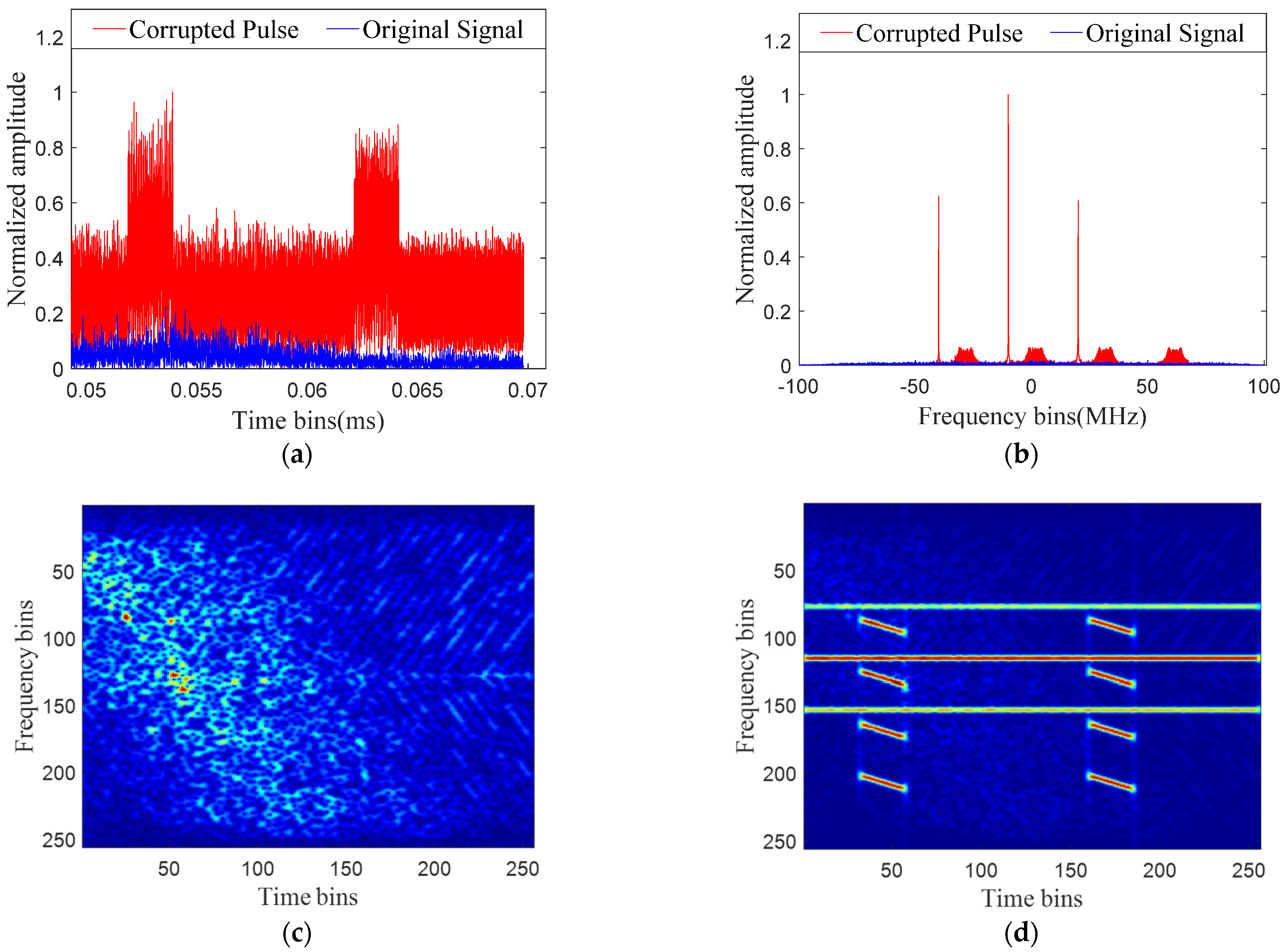
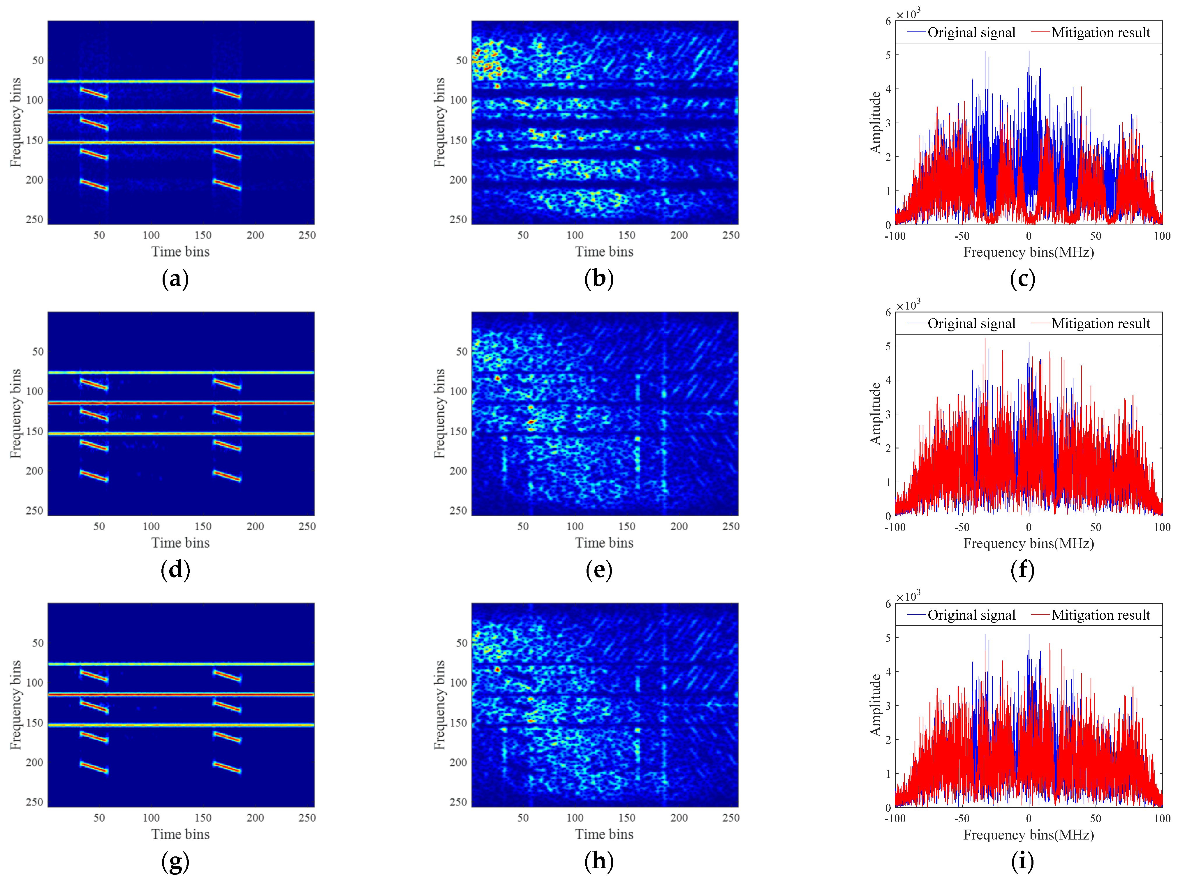
5.1. RFI Mitigation Results of the Simulated Single Snapshot

Firstly, a one-dimensional measured signal with simulated RFI was generated to prove the effectiveness and superiority of the proposed algorithms. Figure 7a,b shows the representation of the SAR echo with and without RFI in the time and frequency domains, respectively. It demonstrates that the envelopes are drastically changed due to the presence of RFI. Figure 7c,d presents the spectrograms of the RFI-free and RFI-contaminated SAR echoes, respectively, in which the characteristics of TES are completely suppressed. Then, different algorithms were utilized to recover the TES.

As discussed above, some parameters including rank and sparsity should be preset before applying the proposed algorithms. The eigenvalue sequence in Figure 8a was obtained by performing eigenvalue decomposition on the spectrogram matrix shown in Figure 7d. As is well known, the eigenvalues reflect the intensities of signal energies and relate to the matrix rank directly. So, the minor large eigenvalues in Figure 8a indicate the low-rank property of RFI. Combined with (33), the rank of the RFI matrix is 23 through the MDL criteria. As for cardinality, ${\epsilon }_1=0.12$ and ${\epsilon }_2=0.4$ are adopted empirically.

To mitigate the RFI in Figure 8, the iterative algorithms were first applied, and the results are shown in Figure 9. Figure 9a,d,g shows the spectrograms of the reconstructed RFI after applying the GoDec, LRDS, and TFC-LRS, respectively. It is clear that LRDS and TFC-LRS have more accurate RFI reconstruction results, whereas GoDec has partially useful signals remaining around the reconstructed RFI. Meanwhile, the RFI reconstructed results shown in Figure 9g show fewer signal residuals than those in Figure 9d, representing the best RFI reconstruction accuracy among these three algorithms.

The recovered TESs after applying the mentioned iterative RFI mitigation algorithms are presented in Figure 9b,e,h, respectively. There are distinct gaps shown in Figure 9b, indicating greater signal loss after applying GoDec. However, as shown in Figure 9e,h, there were no obvious vacant areas and the TES overlapped by the RFI were effectively recovered after applying LRDS and TFC-LRS. Furthermore, Figure 9c,f,i present the spectrum comparison results of the original TES and the recovered TES after applying GoDec, LRDS, and TFC-LRS, respectively. By utilizing LRDS and TFC-LRS, the recovered TES was more similar to the original TES. The divergence between the original TES and the recovered TES obtained by using the GoDec was the largest, and it was smallest after applying TFC-LRS. The comparison in Figure 8 validates the conclusion that the proposed algorithms have better performance due to the more accurate RFI reconstruction model.

Meanwhile, the execution efficiency was analyzed, and the convergence curves of GoDec, LRDS, and TFC-LRS are shown in Figure 10. The convergence curves depict the RFI reconstruction error trend for different RFI mitigation algorithms along the iteration times. The RFI reconstruction error was measured by the root mean square error (RMSE). Obviously, LRDS and TFC-LRS converged after the 14th and 15th iteration, respectively, and the convergence speed was faster than the GoDec. In fact, there was no sign of convergence for GoDec until the maximum iteration number was reached. As discussed above, GoDec has slightly less computational complexity per iteration compared with the proposed algorithms. Therefore, the apparently fewer iterations indicated lower whole computational complexity, which was tested by the time consumption, as shown in

Table 5. Performance comparison of RFI mitigation algorithms for a simulated snapshot.

	Metric	SDR (dB)	SSIM	Time (ms)
Method
ISNF		−5.09	0.75	49.02
ESP		−3.74	0.56	43.74
GoDec		−3.56	0.54	416.63
LRDS		−6.72 1	0.843	144.08
TFD-LRS		−7.10	0.844	194.17
Improvement (%) 2		32.02/79.68/88.76 39.49/89.84/99.44	12.40/50.54/56.11 12.53/50.71/56.30	-/-/65.42 -/-/53.40

¹ The best and the second best results in each metric are highlighted in bold and italics, respectively. ² The two rows denote the improvements of the LRDS and TFC-LRS compared ISNF, ESP, and GoDec, respectively.

.

In pursuit of a more thorough evaluation, non-iterative RFI mitigation algorithms including the ISNF and ESP were applied to compare the performance, and their RFI mitigation results are shown in Figure 11a,b, respectively. It is clear that the RFI was mitigated and the characteristics of TES were recovered to varying degrees. However, there were distinct gaps around the RFI location of the spectrogram after applying ISNF and ESP. This indicates that the RFI mitigation results of the ISNF and ESP had large signal loss. After the visual comparisons shown in Figure 9 and Figure 11 were conducted, it became clear that LRDS and TFC-LRS can achieve better RFI mitigation performances.

In addition to the visual comparison, the quantitative SDR, SSIM, and time consumption metrics obtained by applying the five different RFI mitigation algorithms considered are listed in Table 5. The best and second best values in each metric are highlighted in bold and italics, respectively. The two lines in the improvement row correspond to the percentage increases in the LRDS and TFC-LRS, and the three terms in each row correspond to comparisons with ISNF, ESP, and GoDec, respectively. It is obvious that the proposed RFI mitigation algorithms have the lowest and second lowest SDR, indicating less signal distortion. In addition, they have the best and second best performance in the SSIM metric, which indicates greater consistency with the original TES. It can be concluded that the proposed algorithms exhibit superior performance. As for the time consumption, the proposed algorithms have less expenses than GoDec but more than the non-iterative algorithms including ISNF and ESP. Compared with GoDec, the percentage decreases in time consumption for LRDS and TFC-LRS exceed 65% and 53%, respectively.

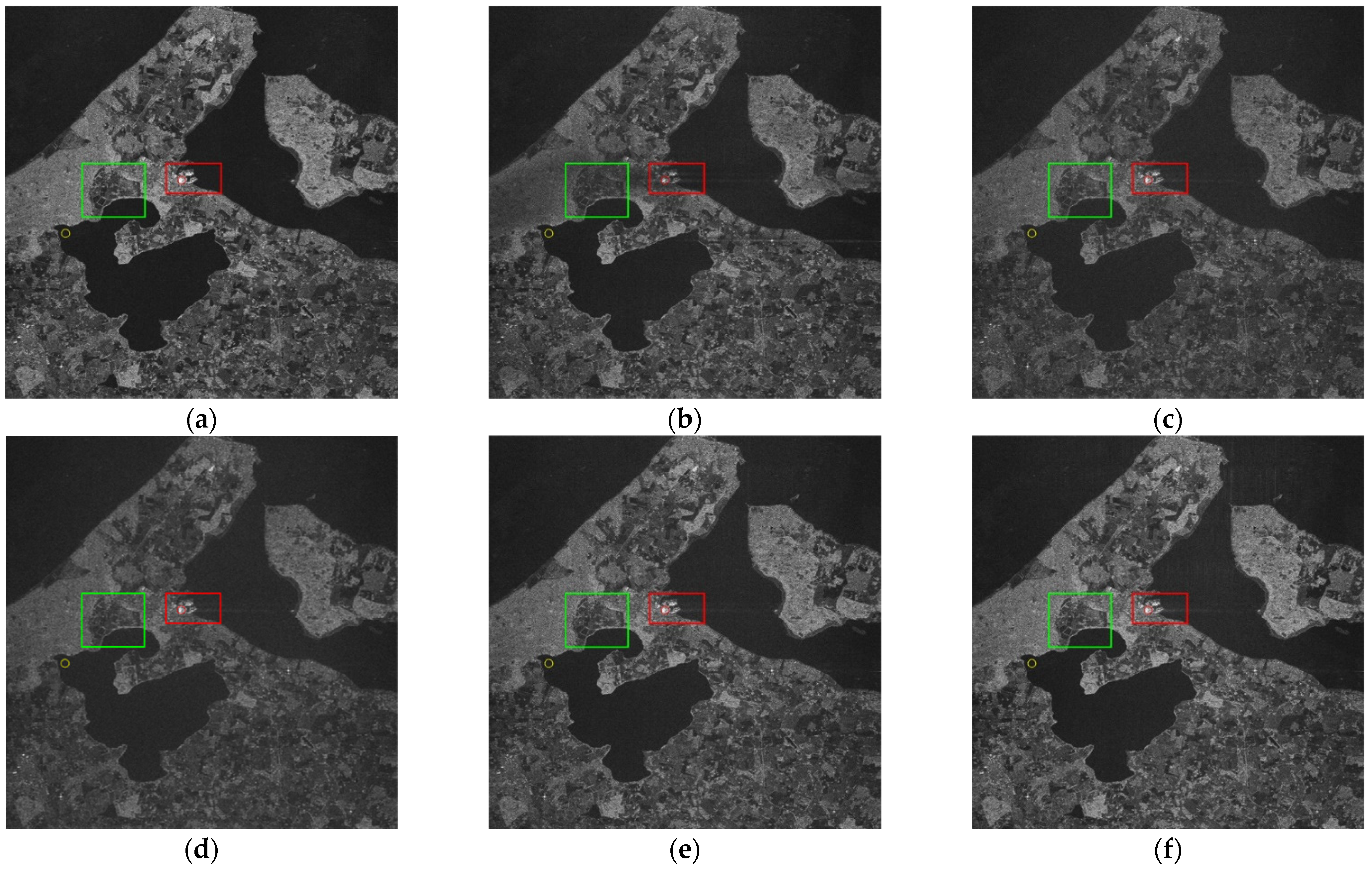
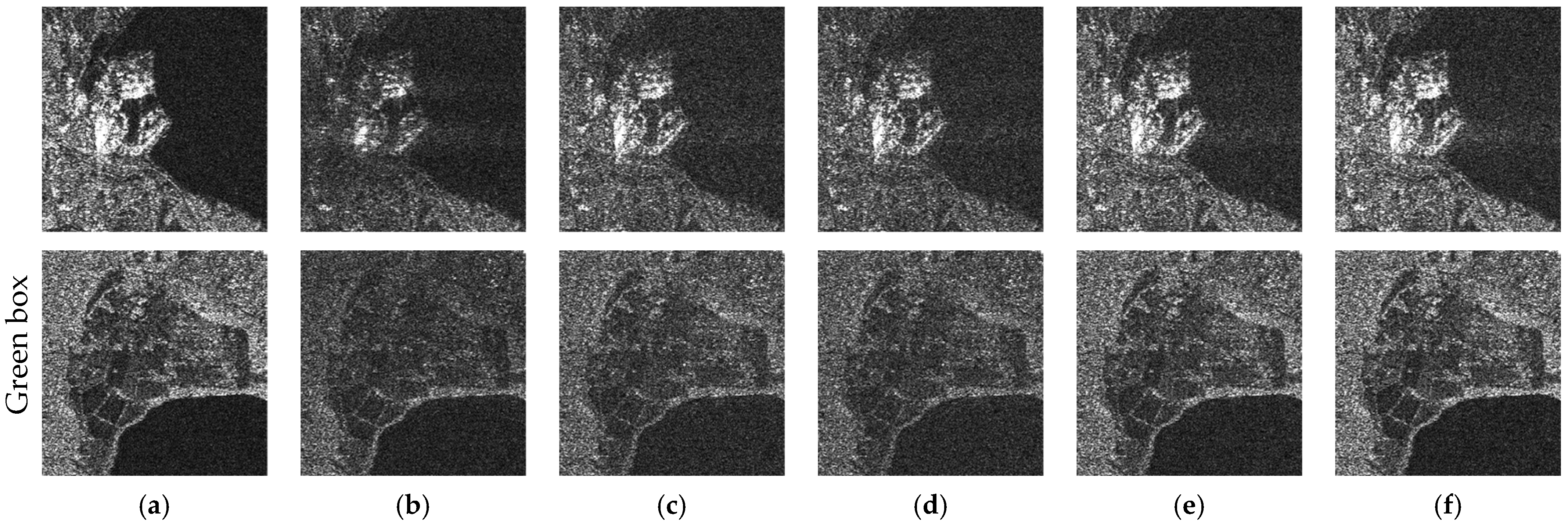
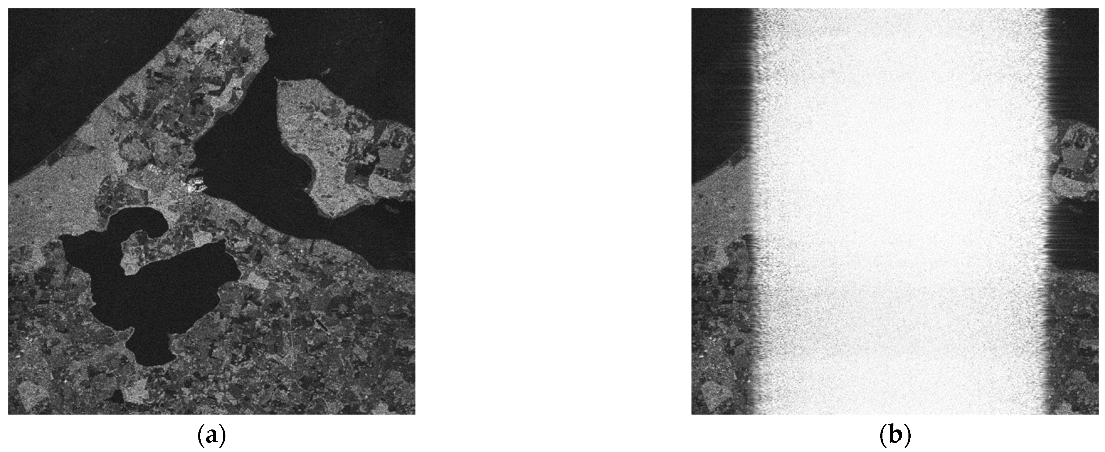
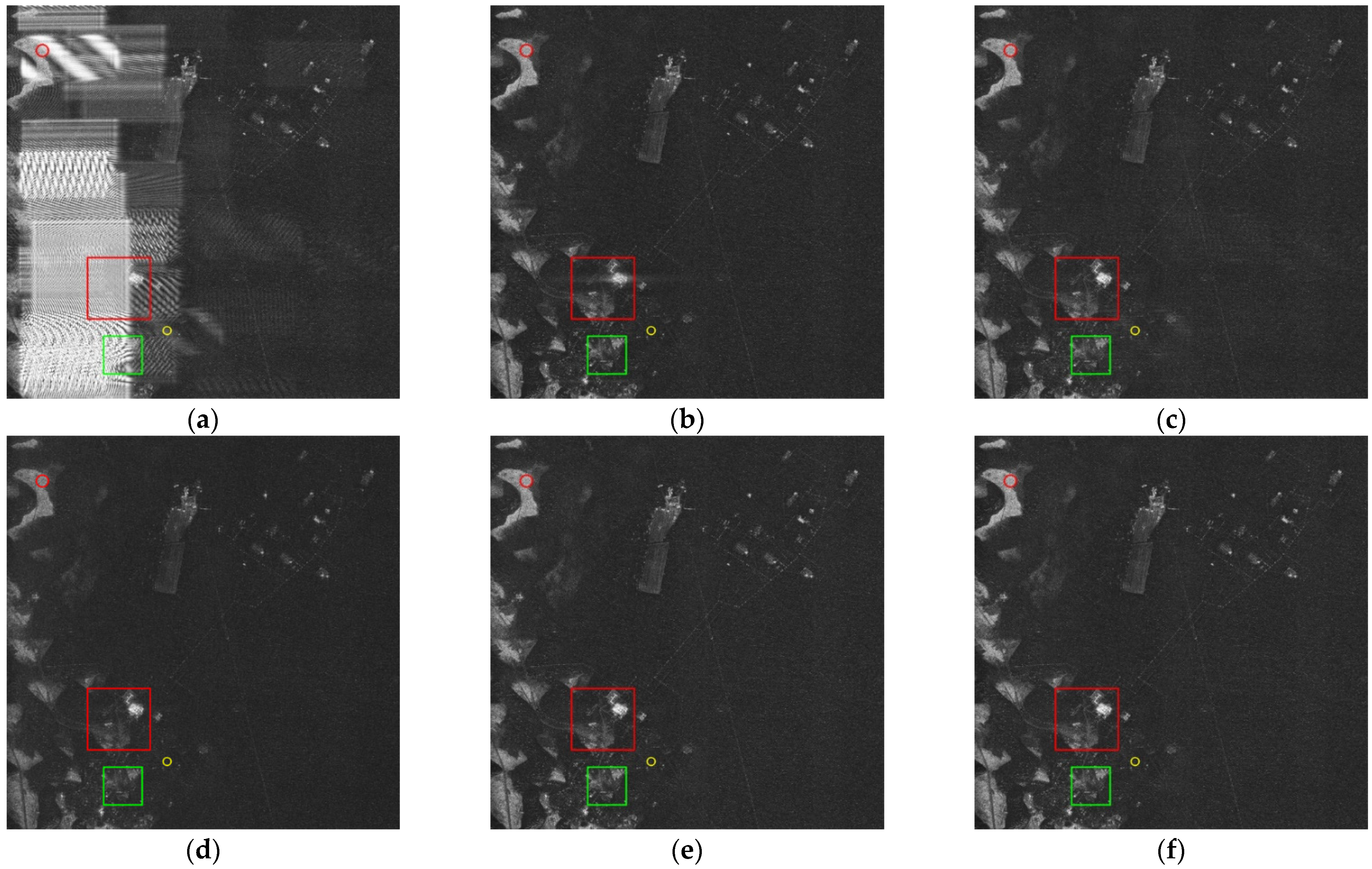
5.2. Mitigation Results of the Measured SAR Data Corrupted with Simulated RFI

Furthermore, the measured SAR scene data with simulated RFI were synthesized and processed by the RFI mitigation algorithms mentioned above to compare the performance. The SAR imaging result of this dataset, shown in Figure 12a, is well-focused and has detailed target features. Meanwhile, Figure 12b presents the SAR imaging result of the same dataset corrupted with the simulated RFI shown in Figure 7. The simulated RFI is modulated randomly along the time and frequency. It is obvious that the RFI seriously hinders the SAR image quality and the subsequent SAR image interpretation.

Firstly, the performance of RFI detection algorithm based on TF skewness was evaluated. The RFI-free SAR dataset was established based on the measured SAR data analysis, and the skewness of each sample was calculated via (5). Then, the curve of the optimal threshold along the different false alarm rates was constructed and found to be monotonically decreasing, as shown in Figure 13a. The RFI threshold was set as 2.298 at a false alarm rate of ${10}^{-3}$. As shown in Figure 13b, the snapshots corrupted with RFI or not were separated precisely by the red dotted line corresponding to the optimal threshold, which was selected from Figure 13a.

Similarly, ISNF, ESP, GoDec, and the proposed algorithms were applied to mitigate the RFI, and the RFI mitigation performances were analyzed. The SAR imaging results obtained after applying the RFI mitigation algorithms mentioned above are presented in Figure 14b–f, respectively, and the scenes marked with different colored boxes are magnified for detailed comparison in Figure 15. A visual inspection of the SAR images shown in Figure 14 indicated that all five RFI mitigation algorithms achieved interference suppression and recovered the original scene. However, the SAR images in Figure 14b–d have poor contrast, and some strong scatter regions are defocused with partial information loss compared with Figure 14a. The SAR imaging results in Figure 14e,f, obtained after applying LRDS and TFC-LRS, are more consistent with the original image. The results demonstrate that there was less information loss and more abundant detailed features after applying the proposed algorithms.

Next, the partial regions were analyzed further to evaluate the details. The magnified SAR images, after applying ISNF (Figure 15b), showed lower contrast and amplitude, which suggests a large signal loss. As for the green boxes corresponding to Figure 15c,d, the edges of vegetation were defective and blurry, indicating the distortion of TES. Therefore, the SAR imaging results obtained after applying LRDS and TFC-LRS presented obviously better performance than those obtained using the other RFI mitigation algorithms.

Beyond the visual comparison, the quantitative evaluation metric values obtained by the five RFI mitigation algorithms are listed in

Table 6. Performance comparison of RFI mitigation algorithms for the measured SAR data with simulated RFI.

	Metric	SSIM	MNR (dB)	Time (s)
Method
ISNF		0.61	−10.22	26.38
ESP		0.56	−11.23	24.99
GoDec		0.51	−11.00	215.63
LRDS		0.75 1	−12.80	71.19
TFD-LRS		0.81	−13.73	85.48
Improvement (%) 2		22.95/33.93/47.06 32.79/44.64/58.82	25.24/13.98/16.36 34.34/22.26/24.82	-/-/66.99 -/-/60.36

¹ The best and the second best results in each metric are highlighted in bold and italic, respectively. ² The two rows denote the improvements of the LRDS and TFC-LRS compared ISNF, ESP, and GoDec, respectively.

. The pixels within the yellow and red circles shown in Figure 14 correspond to the weak region and strong region, respectively. Apparently, the LRDS and TFC-LRS had the highest and second highest SSIM metrics, exceeding those of ISNF, ESP, and GoDec by at least 22% (for LRDS) and 32% (for TFC-LRS). This indicates less signal loss and more abundant details in the SAR images after applying the proposed algorithms. The MNR metrics of the LRDS and TFC-LRS were at least 13% and 22% lower, respectively, compared to the other algorithms, indicating the higher contrast of LRDS and TFC-LRS. Moreover, the time consumption values of LRDS and TFC-LRS were 66.99% and 60.36% lower compared to that of GoDec. Among the three iterative algorithms, LRDS and TFC-LRS were the most efficient. Among all five RFI mitigation algorithms, the LRDS and TFC-LRS achieved superior performance with good effectiveness.

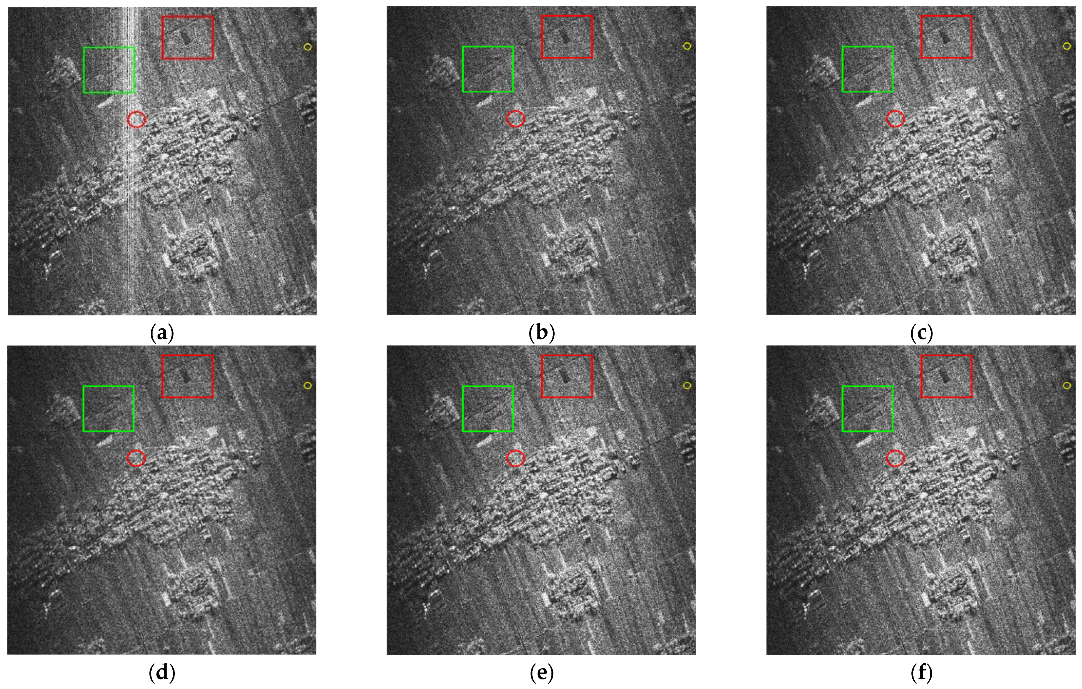
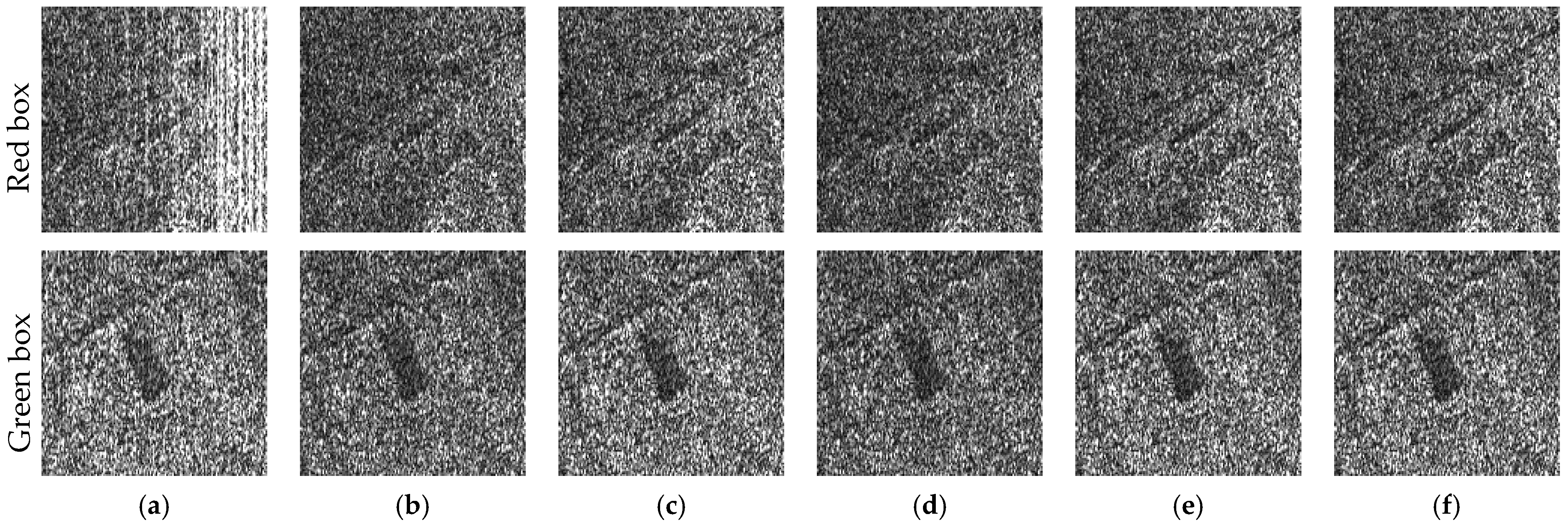
5.3. Mitigation Results of the Measured SAR Data Corrupted with NBI

The above experiments verified the effectiveness and superiority of the proposed RFI mitigation algorithms. Next, the NBI mitigation experiments were conducted on the measured NBI-contaminated SAR data to evaluate the robustness of the proposed algorithms. Figure 16a represents the measured SAR data, which were contaminated by strong NBI in the two-dimensional time domain. The RFI detection results at a false alarm rate of ${10}^{-5}$ are presented in Figure 16b based on the TF skewness detection method.

Based on the prior information offered by RFI detection, the algorithms mentioned in the simulated data experiments were utilized to compare the performance for the measured NBI-corrupted SAR data. Figure 17a is the SAR imaging result without RFI mitigation, where the bright lines overshadow the important target features, such as the buildings and fields. The SAR imaging results obtained after applying ISNF, ESP, GoDec, LRDS, and TFC-LRS are presented in Figure 17b–f, respectively. Although the majority of the NBI was mitigated, some deficiencies were observed in the SAR images when applying ISNF, ESP, and GoDec. By visual comparison, the SAR image of ISNF was found to be blurry around the middle artificial architecture, and it was impossible to extract target features for the subsequent interpretation. Some vestiges of the RFI mitigation procedure can be observed above the artificial building area in Figure 17c,d, indicating signal distortion. Meanwhile, the SAR imaging results obtained after applying LRDS and TFC-LRS were well focused, demonstrating better performance as compared to ISNF, ESP, and GoDec. Similarly, the scenes of red and green boxes are magnified in Figure 18. In summary, the results of the proposed RFI mitigation algorithms were found to have more clear target features and stronger contrast.

After the visual analysis, quantitative evaluation was performed based on the MNR metric and the time consumption listed in

Table 7. Performance comparison of RFI mitigation algorithms for the measured NBI-corrupted SAR data.

	Method	ISNF	ESP	GoDec	LRDS	TFC-LRS	Improvement (%) 2
Metric
MNR (dB)		−7.05	−7.89	−7.44	−7.97 1	−7.94	13.05/1.01/7.12 12.62/0.63/6.72
Time (s)		23.18	23.50	237.97	66.95	55.68	-/-/71.87 -/-/76.60

¹ The best and the second best results in each metric are highlighted in bold and italic, respectively. ² The two rows denote the improvements of the LRDS and TFC-LRS compared ISNF, ESP, and GoDec, respectively.

. In Figure 17, the pixels in the yellow and red circles correspond to the weak region and strong region, respectively. It can be seen that the LRDS and TFC-LRS achieved the lowest and second lowest MNR, with obvious improvements compared to ISNF, ESP, and GoDec. Meanwhile, the time consumption values of LRDS and TFC-LRS were 71.87% and 76.60% less than that of GoDec, respectively. The above analysis results demonstrate that the proposed RFI mitigation algorithms are overall more effective, superior, and efficient.

5.4. Mitigation Results of the Measured SAR Data Corrupted with WBI

Furthermore, the measured WBI-contaminated SAR data were utilized to validate the superiority and robustness of the proposed RFI mitigation algorithms. Figure 19a represents the SAR data in the two-dimensional time domain, and the WBI detection results are shown in Figure 19b at a false alarm rate of ${10}^{-5}$; these results facilitated the following RFI mitigation procedure.

Figure 20a contains the direct SAR imaging result obtained without applying the RFI mitigation algorithm. This SAR image is blurry, and the strong stripes caused by WBI fully suppress the characteristics of the natural and artificial scenes. Figure 20b–f show the imaging results obtained after applying ISNF, ESP, GoDec, LRDS, and TFC-LRS, respectively, where the major WBI was suppressed and the target scene was recovered. However, some misty residual WBI can be observed in the right region of Figure 20c, meaning there was incomplete RFI mitigation. Although there is no residual WBI visible in Figure 20b,d, the SAR images obtained after applying ESP and GoDec were found to be more defocused and blurrier. The target scenes are shown to be even darker in Figure 20d; this was due to the large signal loss. Unlike the SAR images in Figure 20b–d, there are clearer edges and more details in those shown in Figure 20e,f. This shows that the proposed algorithms achieve better RFI mitigation performance compared with ISNF, ESP, and GoDec.

Similarly, some target scenes marked with different colored boxes are magnified for detailed comparison in Figure 21. As for the red box in Figure 21b,d, it can be seen that the target scenes obtained after applying ISNF and GoDec were blurry with large defects in the road features. Furthermore, some residual WBI appeared, as can be seen in the green box of Figure 21c, exhibiting a diffuse target scene. Unlike those RFI mitigation results, the recovered target scenes obtained after applying LRDS and TFC-LRS clearly showed better performance. After the visual inspection, the quantitative MNR and time consumption metrics shown in

Table 8. Performance comparison of RFI mitigation algorithms for the measured WBI-corrupted SAR data.

	Method	ISNF	ESP	GoDec	LRDS	TFC-LRS	Improvement (%) 2
Metric
MNR (dB)		−11.72	−10.28	−11.43	−11.86 1	−12.19	1.19/15.37/3.76 4.01/18.58/6.65
Time (s)		19.45	27.02	101.90	35.97	51.58	-/-/64.70 -/-/49.38

¹ The best and the second best results in each metric are highlighted in bold and italic, respectively. ² The two rows denote the improvements of the LRDS and TFC-LRS compared ISNF, ESP, and GoDec, respectively.

were utilized to evaluate the performance of the five RFI mitigation algorithms. The TFC-LRS and LRDS had the lowest and second lowest MNR values, respectively. This indicates higher contrast in the SAR images after applying the proposed algorithms. Moreover, the time consumption values of LRDS and TFC-LRS were 64.70% and 49.38% lower than that of GoDec, respectively. Therefore, it can be concluded that the proposed RFI mitigation algorithms can achieve superior performance with more effectiveness and efficiencies.

6. Discussion

The RFI mitigation experiment on the simulated single pulse was performed to validate the effectiveness of the proposed RFI mitigation algorithms. As shown in Figure 7, the simulated RFI was found to seriously reduce the SNR and suppress the characteristics of the TES. Firstly, detailed comparisons of the RFI reconstruction results and the recovered TESs, utilizing GoDec, LRDS, and TFC-LRS, are shown in Figure 9. The RFI reconstruction accuracies of LRDS and TFC-LRS were found to be higher than that of GoDec. Meanwhile, the recovered signals obtained after applying LRDS and TFC-LRS were more consistent with the original TES, indicating less signal loss. Figure 10 shows the convergence curves of GoDec, LRDS, and TFC-LRS. It is clear that LRDS and TFC-LRS converged faster than GoDec. Moreover, the non-iterative ISNF and ESP were also utilized to compare the RFI mitigation performance (Figure 11). The large gaps in the spectrograms of the TES recovered by ISNF and ESP indicate serious signal loss, further proving the superiority of the LRDS and TFC-LRS. For more accurate comparison, the quantitative SDR and SSIM metrics were utilized to evaluate the performance of ISNF, ESP, GoDec, LRDS, and TFC-LRS. Table 5 shows that the SDR and SSIM of the proposed RFI mitigation algorithms were improved by at least 32.02% and 12.40%, respectively. This further supports the fact that the proposed RFI mitigation algorithms have better RFI mitigation performance. Meanwhile, LRDS and TFC-LRS were found to have over 53% lower time consumption than GoDec, indicating their faster operation speeds.

To further evaluate the effectiveness and superiority of the proposed RFI mitigation algorithms, the RFI mitigation performances of ISNF, ESP, GoDec, LRDS, and TFC-LRS were analyzed in the image domain. These experiments were based on the measured SAR data superimposed with the simulated RFI, including NBI and WBI. The statistical RFI detection method was validated, as shown in Figure 13. This reveals the effectiveness and robustness of the proposed RFI detection method, with a precise identification result for both NBI and WBI. Then, the SAR imaging results obtained after applying the five mentioned RFI mitigation algorithms are presented in Figure 14. Based on a visual inspection of the SAR images, the images obtained after applying LRDS and TFC-LRS were found to have clearer edges. Meanwhile, Table 6 shows that the quantitative SDR and SSIM metrics of the proposed RFI mitigation algorithms were improved by at least 22.95% and 13.98%, respectively. This indicates that there was less signal loss and distortion in the reconstructed results of the LRDS and TFC-LRS. The time consumption shown in Table 6 demonstrates that the proposed RFI mitigation algorithms are more efficient than GoDec, with a percentage decrease of at least 60.36%.

Beyond the simulated RFI mitigation experiments, the measured RFI-contaminated SAR datasets were employed to verify the robustness of the proposed RFI mitigation algorithms in the experiments described in Section 5.3 (NBI-contaminated data) and 5.4 (WBI-contaminated data). Similarly, the proposed RFI detection method was successfully applied to the measured SAR datasets. The RFI detection results shown in Figure 16 and demonstrate its effectiveness and robustness both for the measured NBI and WBI. Then, the resulting SAR images obtained after applying the five different interference mitigation algorithms are presented in Figure 17 and Figure 20. Through visual inspection, it was found that the images of ISNF, ESP, and GoDec were defocused or blurry, and some even contained residual RFI. On the contrary, clearer edges and better contrast were observed in the SAR imaging results after applying LRDS and TFC-LRS. Meanwhile, the quantitative metric MNR and time consumption for the five algorithms are listed in Table 7 and Table 8. According to the value of MNR, it is clear that the proposed LRDS and TFC-LRS achieved the best and second best performance in both experiments, indicating their stronger robustness and superior performance. Moreover, LRDS and TFC-LRS had significantly better efficiency compared with GoDec because they consumed at least 49% less time.

According to the four experiments, it can be concluded that the proposed RFI mitigation algorithms are more effective and have superior performance compared with the mentioned existing algorithms. Meanwhile, they are more robust for both simulated and measured datasets corrupted with different types of RFI. Moreover, the efficiency of both LRDS and TFC-LRS were found to be greatly improved with faster convergence speeds compared to GoDec.

7. Conclusions

RFI seriously detracts from the SAR imaging quality, which necessitates the development of RFI mitigation algorithms with more accurate models and faster convergence speeds compared to the existing model-driven algorithms. This paper proposes the use of the LRDS and TFC-LRS algorithms to join the low-rank property and the double sparsity property based on the measured SAR data analysis. Firstly, RFI detection was performed by exploiting the fact that the spectrograms of SAR echo with and without RFI have different degrees of Gaussianity. This could be measured by TF skewness, and the adaptive level was improved with the help of the Neyman–Pearson criterion. Then, the LRDS algorithm was introduced to reconstruct the RFI with more precise constraints of structural features for RFI and TES. An alternative iteration strategy combined with the BRP and the soft threshold mapping method was also utilized to optimize the RFI reconstruction model. It improved the accuracy of the RFI reconstruction model and reduced the computational complexity compared with GoDec. Meanwhile, TFC-LRS introduced the TF constraint concept to improve the accuracy of the reconstruction model further. This was inspired by the special sparsity of RFI, which was caused by successive modulation along with time and frequency. The TFC-LRS algorithm could eliminate unnecessary signal loss to yield better performance. With respect to the experiments on both the simulated and measured SAR datasets, the proposed algorithms exhibited more effectiveness, superior performance, and better robustness compared with ISNF, ESP, and GoDec.

References

1. National Academies of Sciences, Engineering, and Medicine. A Strategy for Active Remote Sensing Amid Increased Demand for Radio Spectrum; National Academies Press: Washington, DC, USA, 2015. [Google Scholar]
2. Spencer, M.; Ulaby, F. Spectrum issues faced by active remote sensing. IEEE Geosci. Remote Sens. Mag. 2016, 4, 40–45. [Google Scholar] [CrossRef]
3. Taylor, J. Introduction to Ultra-Wideband Radar Systems; CRC Press: Boca Raton, FL, USA, 1994. [Google Scholar]
4. Meyer, F.J. Performance requirements for ionospheric correction of low-frequency SAR data. IEEE Trans. Geosci. Remote Sens. 2011, 49, 3694–3702. [Google Scholar] [CrossRef]
5. Skriver, H. Crop classification by multitemporal C- and L-band single- and dual-polarization and fully polarimetric SAR. IEEE Trans. Geosci. Remote Sens. 2012, 50, 2138–2149. [Google Scholar] [CrossRef]
6. Moreira, A.; Prats-Iraola, P.; Younis, M.; Krieger, G.; Hajnsek, I. Papathanassiou, K.P. A tutorial on synthetic aperture radar. IEEE Geosci. Remote Sens. Mag. 2013, 1, 6–43. [Google Scholar] [CrossRef] [Green Version]
7. Davis, M.E. Frequency allocation challenges for ultra-wideband radars. IEEE Aerosp. Electron. Syst. Mag. 2013, 28, 12–18. [Google Scholar] [CrossRef]
8. Reigber, A.; Scheiber, R.; Jager, M.; Pau, P.; Hajnsek, I.; Jagdhuber, T. Very-high-resolution airborne synthetic aperture radar imaging: Signal processing and applications. Proc. IEEE 2013, 101, 759–783. [Google Scholar] [CrossRef] [Green Version]
9. Zhou, F.; Tao, M.; Bai, X.; Liu, J. Narrow-band interference suppression for SAR based on independent component analysis. IEEE Trans. Geosci. Remote Sens. 2013, 51, 4952–4960. [Google Scholar] [CrossRef]
10. Tao, M.; Zhou, F.; Liu, J.; Liu, Y.; Zhang, Z.; Bao, Z. Narrow-band interference mitigation for SAR using independent subspace analysis. IEEE Trans. Geosci. Remote Sens. 2014, 52, 5289–5301. [Google Scholar]
11. Su, J.; Tao, H.; Tao, M.; Wang, L.; Xie, J. Narrow-band interference suppression via RPCA-based signal separation in time-frequency domain. IEEE J. Sel. Top. Appl. Earth Obs. Remote Sens. 2017, 10, 5016–5025. [Google Scholar] [CrossRef]
12. Tao, M.; Zhou, F.; Zhang, Z. Wideband interference mitigation in high-resolution airborne synthetic aperture radar data. IEEE Trans. Geosci. Remote Sens. 2016, 54, 74–87. [Google Scholar] [CrossRef]
13. Fan, W.; Zhou, F.; Tao, M.; Bai, X.; Rong, P.; Yang, S.; Tian, T. Interference mitigation for synthetic aperture radar based on deep residual network. Remote Sens. 2019, 11, 1654. [Google Scholar] [CrossRef] [Green Version]
14. Lord, R. Radio frequency interference suppression applied to synthetic aperture radar data. In Proceedings of the 28th General Assembly of the International Union of Radio Science (URSI), New Delhi, India, 23–29 October 2005. [Google Scholar]
15. Dakovic, M.; Thayaparan, T.; Djukanovic, S.; Stankovic, L. Time–frequency-based non-stationary interference suppression for noise radar systems. IEE Radar Sonar Navig. 2008, 2, 306–314. [Google Scholar] [CrossRef] [Green Version]
16. Elgamel, S.; Soraghan, J. Using EMD-FrFT filtering to mitigate very high-power interference in chirp tracking radars. IEEE Signal Process. Lett. 2011, 18, 263–266. [Google Scholar] [CrossRef] [Green Version]
17. Natsuaki, R.; Watanabe, M.; Motohka, T.; Suzuki, S. RFI detection and removal in Range-time Azimuth-frequency domain. In Proceedings of the 2016 IEEE International Geoscience and Remote Sensing Symposium (IGARSS), Beijing, China, 10–15 July 2016; pp. 313–316. [Google Scholar]
18. Liu, Z.; Liao, G.; Yang, Z. Time variant RFI suppression for SAR using iterative adaptive approach. IEEE Geosci. Remote Sens. Lett. 2013, 10, 1424–1428. [Google Scholar] [CrossRef]
19. Zhou, F.; Wu, R.; Xing, M.; Bao, Z. Eigensubspace-based filtering with application in narrow-band interference suppression for SAR. IEEE Geosci. Remote Sens. Lett. 2007, 4, 75–79. [Google Scholar] [CrossRef]
20. Yu, J.; Li, J.; Sun, B.; Chen, J.; Li, C. Multiclass radio frequency interference detection and suppression for SAR based on the single shot multibox detector. Sensors 2018, 18, 4034. [Google Scholar] [CrossRef] [Green Version]
21. Tao, M.; Li, J.; Su, J.; Fan, Y.; Wang, L. Extraction and Analysis of RFI Signatures via Deep Convolutional RPCA. In Proceedings of the General Assembly of the International Union of Radio Science, URSI GASS, Rome, Italy, 28 August–4 September 2021; pp. 1–4. [Google Scholar]
22. Nguyen, L.H.; Ton, T.; Wong, D.; Soumekh, M. Adaptive coherent suppression of multiple wide-bandwidth RFI sources in SAR. In Proceedings of the SPIE 5427, Algorithms for Synthetic Aperture Radar Imagery XI, Orlando, FL, USA, 2 September 2004; pp. 1–16. [Google Scholar]
23. Huang, X.; Liang, D. Gradual RELAX algorithm for RFI suppression in UWB-SAR. Electron. Lett. 1999, 35, 1916–1917. [Google Scholar] [CrossRef]
24. Lord, R.T.; Inggs, M.R. Efficient RFI suppression in SAR using LMS adaptive filter integrated with range/Doppler algorithm. Electron. Lett. 1999, 35, 629–630. [Google Scholar] [CrossRef]
25. Guo, Y.; Zhou, F.; Tao, M.; Sheng, M. A new method for SAR radio frequency interference mitigation based on maximum a posterior estimation. In Proceedings of the General Assembly of the International Union of Radio Science, URSI GASS, Montreal, QC, Canada, 19 August 2017; pp. 1–4. [Google Scholar]
26. Nguyen, L.H.; Tran, T.; Do, T. Sparse models and sparse recovery for ultra-wideband SAR applications. IEEE Trans. Aerosp. Electron. Syst. 2014, 50, 940–958. [Google Scholar] [CrossRef]
27. Liu, H.; Li, D. RFI suppression based on sparse frequency estimation for SAR imaging. IEEE Geosci. Remote Sens. Lett. 2016, 13, 63–67. [Google Scholar] [CrossRef]
28. Lu, X.; Yang, J.; Ma, C.; Gu, H.; Su, W. Wide-band interference mitigation algorithm for SAR based on time-varying filtering and sparse recovery. Electron. Lett. 2018, 54, 165–167. [Google Scholar] [CrossRef]
29. Huang, Y.; Liao, G.; Xu, J.; Li, J. Narrowband RFI suppression for SAR system via efficient parameter-free decomposition algorithm. IEEE Trans. Geosci. Remote Sens. 2018, 56, 3311–3322. [Google Scholar] [CrossRef]
30. Huang, Y.; Liao, G.; Zhang, Z.; Xiang, Y.; Li, J.; Nehorai, A. Fast narrowband RFI suppression algorithms for SAR systems via matrix-factorization techniques. IEEE Trans. Geosci. Remote Sens. 2019, 57, 250–262. [Google Scholar] [CrossRef]
31. Joy, S.; Nguyen, L.; Tran, T.D. Radio frequency interference suppression in ultra-wideband synthetic aperture radar using range-Azimuth sparse and low-rank model. In Proceedings of the 2016 IEEE Radar Conference (RadarConf), Philadelphia, PA, USA, 2 May 2016; pp. 1–4. [Google Scholar]
32. Nguyen, L.; Tran, T. A comprehensive performance comparison of RFI mitigation techniques for UWB radar signals. In Proceedings of the International Conference on Acoustics, Speech, and Signal Process, New Orleans, LA, USA, 5–9 March 2017; pp. 3086–3090. [Google Scholar]
33. Zhou, T.; Tao, D. GoDec: Randomized low-rank & sparse matrix decomposition in noisy case. In Proceedings of the 28th International Conference on Machine Learning (ICML), Bellevue, WA, USA, 28 June–2 July 2011; pp. 33–40. [Google Scholar]
34. Ding, Y.; Fan, W.; Zhou, F. Wideband Interference Mitigation for Synthetic Aperture Radar Data Based on Variational Bayesian Inference. In Proceedings of the General Assembly of the International Union of Radio Science, URSI GASS, Rome, Italy, 29 August–5 September 2020; pp. 1–4. [Google Scholar]
35. Ding, Y.; Du, J.; Zhang, Z.; Fan, W.; Zhou, F. Radio Frequency Interference Mitigation Method for Synthetic Aperture Radar Using Joint Low Rank and Sparsity Property. In Proceedings of the General Assembly of the International Union of Radio Science, URSI GASS, Rome, Italy, 28 August–4 September 2021; pp. 1–4. [Google Scholar]
36. Miller, T.; Potter, L.; McCorkle, J. RFI suppression for ultra wideband radar. IEEE Trans. Aerosp. Electron. Syst. 1997, 33, 1142–1156. [Google Scholar] [CrossRef]
37. Zhao, Z.; Wang, Z.; Shi, X. FM interference suppression for PRC-CW radar based on adaptive STFT. In Proceedings of the International Symposium on Microwave, Antenna, Propagation and EMC Technologies for Wireless Communications (MAPE), Beijing, China, 27–29 October 2009; pp. 84–88. [Google Scholar]
38. Zhang, S.; Xing, M.; Guo, R.; Zhang, L.; Bao, Z. Interference suppression algorithm for SAR based on time–frequency transform. IEEE Trans. Geosci. Remote Sens. 2011, 49, 3765–3779. [Google Scholar] [CrossRef]
39. Dandawate, A.V.; Giannakis, G.B. Asymptotic properties and covariance expressions of kth-order sample moments and cumulants. In Proceedings of the Asilomar Conference on Signals, Systems, and Computers, Pacific Grove, CA, USA, 1–3 November 1993; pp. 1186–1190. [Google Scholar]
40. Richards, M.A. Fundamentals of Radar Signal Processing; McGraw-Hill: New York, NY, USA, 2005. [Google Scholar]
41. Mertins, A.; Mertins, D.A. Signal Analysis: Wavelets, Filter Banks, Time–Frequency Transforms and Applications; Wiley: New York, NY, USA, 1999. [Google Scholar]
42. Rajapakse, J.C. Adaptive Blind Signal and Image Processing: Learning Algorithms and Applications; Wiley: New York, NY, USA, 2002. [Google Scholar]
43. Wang, J.; Huang, T.; Zhao, X.; Jiang, T.; Ng, M. Multi-Dimensional Visual Data Completion via Low-Rank Tensor Representation Under Coupled Transform. IEEE Trans. Image Process. 2021, 30, 3581–3596. [Google Scholar] [CrossRef]
44. Skolnik, M.I. Radar Handbook, 3rd ed.; McGraw-Hill: New York, NY, USA, 2008. [Google Scholar]
Figure 1. Classification diagram of RFI mitigation algorithms.
Remotesensing 14 00775 g001
Figure 2. Flowchart of the proposed algorithms incorporating the SAR imaging process. ① and ② present the RFI reconstruction models of LRDS and TFC-LRS, respectively. A complete RFI mitigation procedure in SAR system should contain the data preprocessing, RFI detection, RFI reconstruction, RFI cancellation, and SAR imaging.
Remotesensing 14 00775 g002
Figure 3. Statistical analysis of SAR echo spectrograms: (a) RFI-free signal; (b) WBI-corrupted signal; (c) NBI-corrupted signal; and (df) histograms and skewness, respectively, corresponding to (ac). It is easy to see that the NBI concentrates in several frequency points while WBI occupies a larger frequency band. Furthermore, they all gather in limited regions with the higher amplitude in the spectrogram, which increases the value of TF skewness.
Remotesensing 14 00775 g003
Figure 4. The skewness histogram of the RFI-free SAR dataset.
Remotesensing 14 00775 g004
Figure 5. Structural analysis of RFI in the TF domain: (a,d), spectrograms of SAR echoes contaminated with NBI and WBI, respectively; (b,e), Eigenvalue sequences corresponding to (a,d), respectively; (c,f), amplitude analyses for (a,d), respectively.
Remotesensing 14 00775 g005
Figure 6. Structural analysis of TES in the TF domain: (a) TF spectrograms of TES; (b) amplitude analysis result corresponding to (a).
Remotesensing 14 00775 g006
Figure 7. Representations of the simulated RFI-contaminated SAR echo signal. (a,b), the RFI-corrupted SAR echo in the time and frequency domains, respectively; (c) original RFI-free signal; and (d) RFI-contaminated SAR echo in the TF domain.
Remotesensing 14 00775 g007
Figure 8. Eigenvalues and MDL curve of the spectrogram in Figure 7d: (a) the eigenvalue sequence; (b) the MDL function curve of (a).
Remotesensing 14 00775 g008
Figure 9. Analysis of the mitigation results. (a,d,g), the spectrograms of reconstructed RFI after applying GoDec, LRDS, and TFC-LRS, respectively. (b,e,h), the spectrograms of recovered TES after applying GoDec, LRDS, and TFC-LRS, respectively. (c,f,i) comparison of the spectrums of the original TES and the recovered TES after applying GoDec, LRDS, and TFC-LRS, respectively.
Remotesensing 14 00775 g009
Figure 10. The convergence curves of the root mean square error when utilizing GoDec, LRDS, and TFC-LRS.
Remotesensing 14 00775 g010
Figure 11. Spectrograms of the results after applying (a) ISNF and (b) ESP.
Remotesensing 14 00775 g011
Figure 12. SAR image of the measured data (a) without RFI and (b) corrupted with simulated RFI.
Remotesensing 14 00775 g012
Figure 13. RFI detection results of the measured SAR data corrupted with simulated RFI: (a) the variation of optimal threshold with different false alarm levels. (b) the RFI detection result at a false alarm rate of 10 3 .
Remotesensing 14 00775 g013
Figure 14. Resulting SAR image after applying (a) the SAR imaging algorithm applied directly for the measured SAR data, (b) ISNF, (c) ESP, (d) GoDec, (e) LRDS, and (f) TFC-LRS.
Remotesensing 14 00775 g014
Figure 15. Comparison of the enlarged areas in Figure 14: (Row 1) the red box region; (Row 2) the green box region. (a) The RFI-free SAR image, (b) ISNF, (c) ESP, (d) GoDec, (e) LRDS, and (f) TFC-LRS.
Remotesensing 14 00775 g015
Figure 16. The NBI detection results on the measured SAR data corrupted with NBI: (a) the NBI contaminated SAR data in the two-dimensional time domain; (b) the NBI detection results of (a) via the TF skewness detection algorithm.
Remotesensing 14 00775 g016
Figure 17. Resulting SAR image after applying (a) the SAR imaging algorithm applied directly for the original data, (b) ISNF, (c) ESP, (d) GoDec, (e) LRDS, and (f) TFC-LRS.
Remotesensing 14 00775 g017
Figure 18. Comparison of the enlarged areas in Figure 17. (Row 1): the red box region; (Row 2) the green box region. (a) The RFI-free SAR image, (b) ISNF, (c) ESP, (d) GoDec, (e) LRDS, and (f) TFC-LRS.
Remotesensing 14 00775 g018
Figure 19. The WBI detection results on the measured SAR data corrupted with WBI: (a) the WBI-contaminated data in the two-dimensional time domain; (b) the WBI detection results via the TF skewness detection algorithm.
Remotesensing 14 00775 g019
Figure 20. Resulting SAR image after applying (a) the SAR imaging algorithm applied directly without interference mitigation, (b) ISNF, (c) ESP, (d) GoDec, (e) LRDS, and (f) TFC-LRS.
Remotesensing 14 00775 g020
Figure 21. Comparison of the enlarged areas in Figure 20: (Row 1) the red box region; (Row 2) the green box region. (a) The RFI-free SAR image, (b) ISNF, (c) ESP, (d) GoDec, (e) LRDS, and (f) TFC-LRS.
Remotesensing 14 00775 g021