Pix2pix Conditional Generative Adversarial Network with MLP Loss Function for Cloud Removal in a Cropland Time Series

Abstract

Clouds are one of the major limitations to crop monitoring using optical satellite images. Despite all efforts to provide decision-makers with high-quality agricultural statistics, there is still a lack of techniques to optimally process satellite image time series in the presence of clouds. In this regard, in this article it was proposed to add a Multi-Layer Perceptron loss function to the pix2pix conditional Generative Adversarial Network (cGAN) objective function. The aim was to enforce the generative model to learn how to deliver synthetic pixels whose values were proxies for the spectral response improving further crop type mapping. Furthermore, it was evaluated the generalization capacity of the generative models in producing pixels with plausible values for images not used in the training. To assess the performance of the proposed approach it was compared real images with synthetic images generated with the proposed approach as well as with the original pix2pix cGAN. The comparative analysis was performed through visual analysis, pixel values analysis, semantic segmentation and similarity metrics. In general, the proposed approach provided slightly better synthetic pixels than the original pix2pix cGAN, removing more noise than the original pix2pix algorithm as well as providing better crop type semantic segmentation; the semantic segmentation of the synthetic image generated with the proposed approach achieved an F1-score of 44.2%, while the real image achieved 44.7%. Regarding the generalization, the models trained utilizing different regions of the same image provided better pixels than models trained using other images in the time series. Besides this, the experiments also showed that the models trained using a pair of images selected every three months along the time series also provided acceptable results on images that do not have cloud-free areas.

1. Introduction

To ensure global food security, which is one of the seventeen sustainable development goals defined by the United Nations to be accomplished by 2030, the United Nations [1] states that is essential to decrease food loss and waste, as well as increase sustainable agriculture production [2,3]. In this regard, decision-makers need high-quality agriculture statistics to develop strategies and policies to expand sustainable food production [4]. The remote sensing community has been making efforts to develop methods to extract agricultural statistics from remote sensing images [4,5]. Researchers and groups such as the Joint Experiment for Crop Assessment and Monitoring (JECAM) (jecam.org/) and the Global Agricultural Monitoring Community (GEOGLAM) (earthobservations.org/geoglam) have addressed the acquisition of agricultural statistics in regional and global scales through satellite images [2,6]. However, despite all efforts, clouds are still a hindrance for crop monitoring with optical satellite images. According to Whitcraft et al. [7], cloud cover is one of the major limitations for applications such as crop type mapping, crop condition monitoring and forecasting crop yield, as they require multi-temporal images, sometimes every week or even more frequently. On average, about 55% of the Earth’s land surface is covered by clouds [8]. In South America, cropland areas can have up to 80% cloud cover frequency during the rainy season from December to February, making agricultural monitoring through optical satellite images challenging in this region [9]. Therefore, to deliver high-quality agricultural statistics using multi-temporal optical satellite images, it is essential to develop methods for cloud removal in satellite images [10].

Due to this need, techniques to reconstruct missing information in remote sensing images is a highly relevant research topic. Shen et al. [11] addressed this issue in a broad technical review. Li et al. [12], Melgani [13], Benabdelkader et al. [14], Benabdelkader et al. [15] and Gómez-Chova et al. [16] addressed cloud removal with approaches that build cloud-free image composites selecting cloud-free pixels in images collected along a short period. Despite these approaches proving visually high-quality images, they did not meet the high temporal frequency needed for many agricultural applications. Shao et al. [17] evaluated different smoothing algorithms to perform data cleaning in satellite optical image time series. Even while this approach is able to remove thick clouds and cloud shadows, some noises may not be removed, and new noises may appear in cloud-free regions if they occur in previous and subsequent images from the time series [18].

In the past few years, since Goodfellow et al. [19] presented the Generative Adversarial Network (GAN), it became the mainstream approach to address cloud removal, with different versions of GAN being used in image translation tasks. Enomoto et al. [20], Bermudez et al. [21], and Grohnfeldt et al. [22] addressed cloud removal using a conditional GAN (cGAN) trained to learn a nonlinear mapping function to translate SAR images into cloud-free optical images. This approach takes advantage of the fact that SAR images have almost no influence from atmospheric conditions. However, although this approach is able to generate plausible cloud-free images, it has issues with fine objects as well as with the spectral information in the generated images, since differences with the real images can be noticed in the synthetic images. Sing et al. [23] trained a cycle-GAN to perform cloud removal in RGB images. Although this approach does not require SAR images or other input data, it works just to remove thin clouds, failing to address cloud removal in images with thick clouds. Bermudez et al. [24] proposed to use a temporal constraint in the cGAN. The main idea was to use a SAR image as conditioning data in the cGAN as well as a cloud-free optical image collected one year before the image to be generated. The synthetic images were visually similar to the real ones; however, some differences could be noticed that likely came from assumption that the classes in the image to be generated were almost identical to the optical image collected in the previous year, which can be a drawback for tropical cropland monitoring as they have high crop dynamics [25]. Li et al. [26] adapted the pix2pix cGAN presented by Isola et al. [27] adding to its original loss function a new term referring to the structural similarity index measure (SSIM) with the aim to generate synthetic images close to the ground truth. In general, this approach achieved satisfactory results for most of the classes, although, despite the cropland borders being well defined, the color information in the synthetic images was not as similar to the ground truth as expected. Turnes et al. [28] presented the atrous-cGAN to perform SAR on optical image translation. As atrous convolutions and atrous spatial pyramid pooling (ASPP) can deal with the loss of high-frequency information that is usual in U-nets, they adapted the original pix2pix cGAN with atrous convolutions and ASPP modules to improve fine details in optical synthetic images. Regarding the visual analysis and semantic segmentation, the results were better than the original pix2pix cGAN; however, it lacked a detailed color analysis for the classes in the datasets.

The spectral response plays a key role in the semantic segmentation of remote sensing images; it is particularly important in tasks in which classes have similar spectral characteristics, such as crop type mapping. Regardless of the approach used to address image translation or cloud removal in the aforementioned studies, there appear differences in the pixel values between the synthetic and real images that should be diminished to improve crop type mapping.

For this matter, this study has the following hypothesis: “The addition of a custom loss function which minimizes the distance between the semantic segmentation for the real and synthetic image to the traditional pix2pix cGAN objective function, may deliver spectral information which may also improve crop type mapping in areas covered by cloud and cloud shadows in optical satellite images”. The additional constraint proposed is the L1-distance between the semantic segmentation for the real and synthetic images, enforcing the synthetic pixels to have a value that can be used to assign them to the right class. It was proposed to perform the semantic segmentation using a Multi-Layer Perceptron Network designed with the Particle Swarm Optimization (PSO) algorithm [29], as the combination of the metaheuristics and deep learning has provided impressive results in different areas. For instance, Rodrígues-de-la-Cruz et al. [30] presented an algorithm based on Particle Swarm Optimization (PSO) to design a GAN to generate medical images; Bacanin et al. [31] developed an algorithm to perform the hyper-parameters optimization of a convolutional neural network, aiming to improve brain tumor classification in medical images; and Zhang and Zhao [32] used PSO to have more stability and avoid mode collapse, which is usual in GAN.

Most of the crop mapping approaches are carried out with optical image time series; therefore, performing a cloud removal in the sequence of images is usually needed. As GANs comprehend two neural networks which usually are deep convolutional neural networks, training these models demand high computational cost, making it unfeasible to train a model for every image in the satellite image time series. Another matter is that for some periods of the year (e.g., rainy season) there are no cloud-free areas to perform the training of a model. Thereby, it was also evaluated whether models trained from few images along the time series could provide plausible synthetic pixels for other images. To the best of our knowledge, this is the first time that generalization is addressed in a generative model aiming to fill cloud-cover gaps along satellite image time series. Therefore, the two objectives of this study were to:

• Investigate whether extending the original pix2pix cGAN objective function with a custom loss function that minimizes the distance between the semantic segmentation of the real and synthetic images, could deliver synthetic pixels that improve crop type mapping with optical remote sensing images covered by clouds and cloud shadows;
• Evaluate the generalization for generative models, meaning, whether models trained in few images selected along the time series could provide suitable synthetic pixels for cloud-covered areas on other images along the same satellite image time series.

This article is organized as follows. Section 2 presents a brief overview of the GAN and its extension, cGAN, as well as the pix2pix cGAN. Section 3 introduces the proposed custom loss function to be added to the pix2pix cGAN. Section 4 presents the dataset, the satellite images pre-processing, experiments description, performance assessment, as well as the networks architecture used to address the study. Section 5 reports the results achieved in the experiments carried out. Section 6 discusses the results in relation to other studies. Finally, Section 7 presents the final remarks and conclusions, pointing to future work.

2. Background

2.1. Generative Adversarial Network

Generative Adversarial Networks embraces two neural networks competing against each other, a Generative Neural Network (G) and a Discriminative Neural Network (D). G is a non-linear function that learns to map a random noise vector (z) to produce an output (y), as in Equation (1):

G: z→y.

(1)

The data distribution of the output, $p_z\left(z\right)$, must be as close as possible of the data distribution from the input (real data) ($x$), $p_x\left(x\right)$. D is a network that discriminates if its input is real or fake, so if the input comes from $p_x\left(x\right)$ or $p_z\left(z\right)$.

The main goal of a GAN is to improve G until D cannot tell if generated images are real or synthetic. To this end, the models are trained in an adversarial manner in a zero-sum game, trying to find the optimal mapping function, Equation (2):

$$G^{*}=\arg \underset{G}{\min }\underset{D}{\max }{\mathcal{L}}_{GAN}\left(G,D\right),$$

(2)

where ${\mathcal{L}}_{GAN}\left(G,D\right)$ is the objective function, Equation (3):

$${\mathcal{L}}_{GAN}\left(G,D\right)={\mathbb{E}}_{x~p_x\left(x\right)}\left[\log D\left(x\right)\right]+{\mathbb{E}}_{z~p_z\left(z\right)}\left[\log (1-D\left(G\left(z\right)\right))\right],$$

(3)

where $x$ is the real data vector; $p_x$ is the probability distribution of the real data; $z$ is the random noise vector; and $p_z$ is the probability distribution of the noise data.

The training of GAN is performed alternating D and G training, towards a gradual improvement of both. The aim is to not improve too much one that will make the other fail. The backpropagation algorithm is used to carry out the training. First, D and G are initiated with random initial weights, then D is trained with real and synthetic samples while G is set as not trainable (fixed). After updating D weights, it is set as not trainable and G is updated to minimize the loss from D, considering now that the output of the G as “real samples”.

2.2. Conditional Generative Adversarial Network

Mirza and Osindero [33] introduced the conditional GAN which is an extension of the GAN presented above. The main difference is that the generative and discriminate networks have their outputs conditioned on extra information, like an observed image ($u$). So, the G can learn to map a random noise vector ($z$) and observed image ($u$), to produce an output ($y$), Equation (4):

$$G:\left\{z, u\right\} \to y.$$

(4)

The objective function of cGAN is expressed in Equation (5):

$${\mathcal{L}}_{cGAN}\left(G,D\right)={\mathbb{E}}_{x~p_x\left(x\right)}\left[\log D\left(x,u\right)\right]+{\mathbb{E}}_{z~p_z\left(z\right)}\left[\log (1-D\left(G\left(z, u\right)\right)\right].$$

(5)

2.3. Pix2pix Conditional Generative Adversarial Network

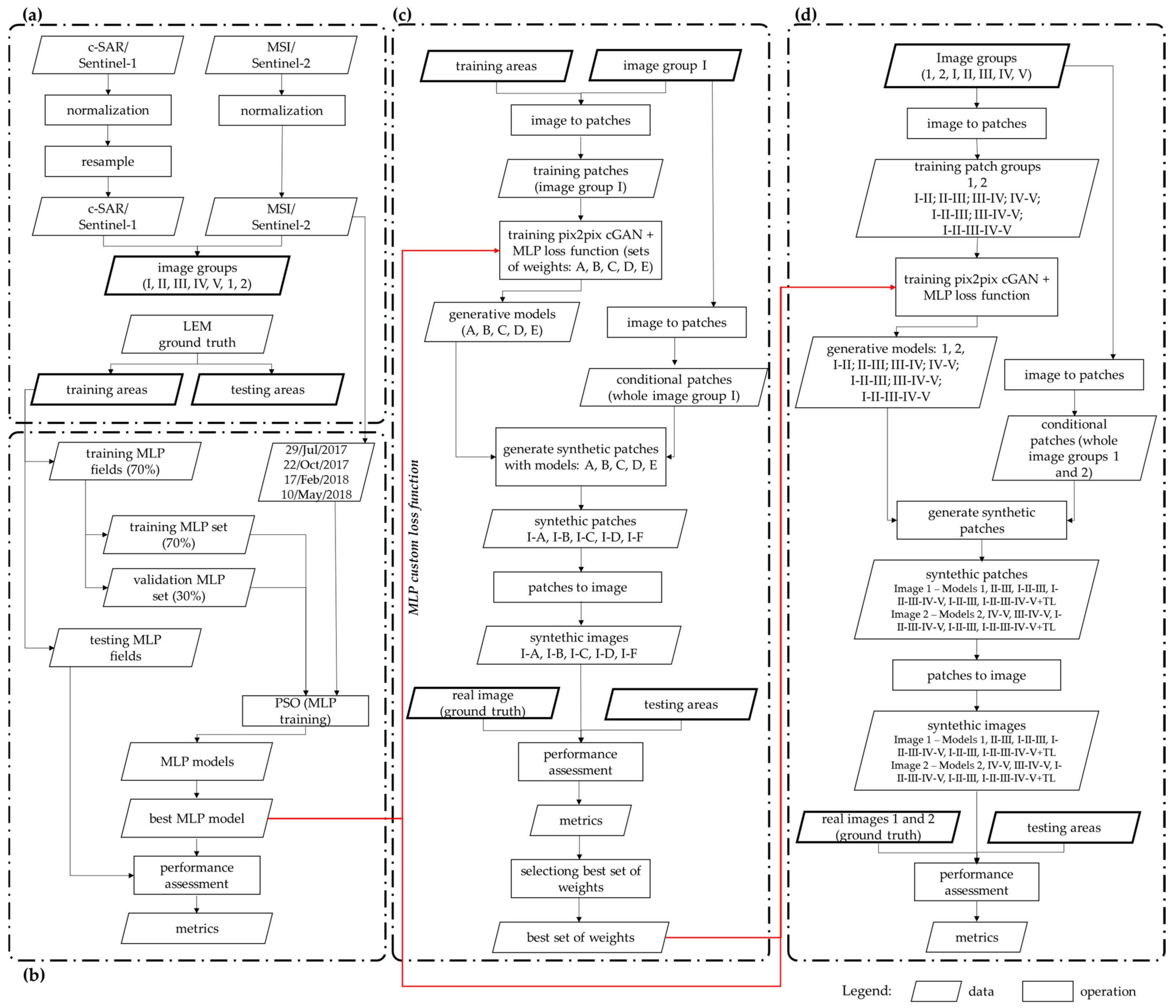
Goodfellow et al. [19] proposed GAN with a discriminator that is updated with a loss function that outputs if the synthetic image is real or not, while the generator has its weights updated through the same loss function but with the discriminator fixed, as described in Section 2.1. Despite this approach working reasonably, frequently it provides blurred images. In this regard, different studies have addressed the GAN loss function, aiming to improve the quality of the output images. An alternative is to combine the adversarial loss with the distance between the ground truth (real images) and synthetic images. Then the generator is updated via a weighted sum of both metrics as presented in Equation (6):

$$G^{*}=arg \underset{G}{min} \underset{D}{max} {\lambda }_{cGAN}{\mathcal{L}}_{cGAN}\left(G,D\right)+{\lambda }_d{\mathcal{L}}_d\left(G\right),$$

(6)

where ${\mathcal{L}}_{cGAN}$ is the adversarial loss; ${\mathcal{L}}_d$ is the loss function based on some metric between the ground truth and synthetic image; and ${\lambda }_{cGAN}$ and ${\lambda }_d$ are the weights of each loss function. This approach makes the generator produce more plausible images with respect to the input image, and not just in respect to the target domain.

Based on this idea, different studies have combined different distance metrics to the cGAN objective function to perform image translation tasks. Pathak et al. [34] used the L2-distance, Equation (7):

$${\mathcal{L}}_{L2}={\mathbb{E}}_{x~p_x\left(x\right)}\left[{\left(x-G\left(u\right)\right)}^2\right],$$

(7)

to reconstruct missing image parts. Isola et al. [27] proposed the pix2pix cGAN using the L1-distance, Equation (8):

$${\mathcal{L}}_{L1}={\mathbb{E}}_{x~p_x\left(x\right)}\left[\Vert x-G\left(u\right){\Vert }_1\right],$$

(8)

in different image translation tasks, while Enomoto et al. [20], Bermudez et al. [21] and Bermudez et al. [24] used the pix2pix cGAN in a remote sensing context to translate SAR to optical images. In Equations (7) and (8), $x$ is the ground truth; and $G\left(u\right)$ is the synthetic image using as condition the input data $\left(u\right)$.

3. Proposed Method

Bermudez et al. [24] followed previous studies using the original pix2pix cGAN, where it combines the adversarial loss function with the L1-distance between the real and synthetic images. To improve the quality of the generated images, they also constrained the output images using a temporal condition, where the synthetic optical image (y) was conditioned in a SAR image taken on a date as close as possible to the date of y, as well as in a SAR image and a cloud-free optical image taken during the same period of the year, but one year before of y. In this approach, they consider that the classes do not change or they have a minimum change from the previous year to the next.

This study followed the temporal constraint proposed by Bermudez et al. [24]; however, this research used only an almost-cloud-free optical image taken as close as possible to the image to be generated as temporal condition. Therefore, considering that the optical image (objective image) which was desired to remove cloud areas was taken at the date $t_i$ the cGAN was conditioned in SAR image taken at $t_i$ (or as close as possible) and in an optical image taken at $t_{i-1}$ or $t_{i+1}$ or as close as possible.

The L1-distance was used following previous studies, like that of Isola et al. [27] which introduced the pix2pix cGAN, as well as studies which addressed cloud removal in remote sensing imagery with the pix2pix cGAN, like Bermudez et al. [21,24] and Enomoto et al. [20], among others. Minimizing the L1-distance between the real and synthetic images is mainly related to the shape of objects, and therefore used to make the generated image less blurred. To enforce the generated pixel values to be similar to the real optical image for the same targets, it was proposed an additional constraint to the loss function. The additional constraint is to use the L1-distance between the semantic segmentation from the real and generated images, enforcing the synthetic pixels to have values that enhances the semantic segmentation afterwards. So, the authors added the L1-distance between the semantic segmentation of the ground truth and synthetic images to the loss function presented previously. To perform the semantic segmentation in the loss function, the authors used a Multi-Layer Perceptron (MLP) network. The objective function of the proposed method is presented in Equation (9):

$$G^{*}=\arg \underset{G}{\min } \underset{D}{\max }{\lambda }_{cGAN}{\mathcal{L}}_{cGAN}\left(G,D\right)+{\lambda }_{L1}{\mathcal{L}}_{L1}\left(G\right)+{\lambda }_{MLP}{\mathcal{L}}_{MLP}\left(G\right),$$

(9)

where ${\lambda }_{L1}$ and ${\mathcal{L}}_{L1}$ are the weight and the L1-distance between the ground truth and synthetic images; ${\lambda }_{MLP}$ and ${\mathcal{L}}_{MLP}$ are the weight and L1-distance between the semantic segmentation of the ground truth and synthetic images produced using an MLP network. The last term of Equation (9) can be written as presented in Equation (10):

$${\mathcal{L}}_{MLP}={\mathbb{E}}_{x~p_x\left(x\right)}\left[\Vert MLP\left(x\right)-MLP\left(G\left(u\right)\right){\Vert }_1\right],$$

(10)

where $x$ is the ground truth; and $G\left(u\right)$ is the synthetic image using as condition the input data ($u$).

4. Material and Methods

A diagram of the study is presented in Figure 1. The four main phases of the process include: (a) the dataset and satellite image pre-processing, (b) the MLP hyper-parameter optimization, (c) the evaluation of the MLP custom loss function, and (d) the evaluation of the generalization capability for the generative models. The first phase addresses the ground truth and satellite images as well as the pre-processing. The MLP hyper-parameter optimization phase presents the approach for optimizing the parameters of the classifier used in the custom loss function as well as its training. In the evaluation of the MLP custom loss function, it was used the best MLP trained in the previous phase to perform the training of different pix2pix cGAN with the MLP loss function and different sets of weights for the MLP loss function. Finally, to perform the evaluation of the generative models generalization, it was used the best set of weights selected through the previous step to train different models using different sets of images selected along the time series. Details on each step are provided in the following subsections.

4.1. Dataset and Satellite Image Pre-Processing

The experiments were performed using the Luís Eduardo Magalhães (LEM) (Bahia State, Brazil) benchmark for tropical agricultural remote sensing application [35]. The LEM database has optical and Synthetic Aperture Radar (SAR) images, along with 794 polygons for crop fields. Used in this study were the optical Sentinel-2 multispectral reflectance images and the C-SAR/Sentinel-1 backscatter coefficient images in dB scale.

Each polygon in the ground truth has as attributes the monthly land use (crop type) for 2017/2018 harvests. The classes include millet, pasture, wheat, cerrado (Brazilian savanna), corn + crotalaria, beans, soybean, crotalaria, eucalyptus, grass, maize, non-commercial crops, unidentified, cotton, sorghum, hay, conversion area, uncultivated soil and coffee. As depicted in Figure 1a, the ground truth was divided into training and testing fields. The boundaries of Luís Eduardo Magalhães municipality as well as the crop fields for the training and testing are shown in Figure 2.

The pixel values of the optical and SAR images were normalized to have their values between −1 and 1. The optical images were normalized by linear mapping using the Python scikit-learn package [36]. The SAR images were normalized using the approach presented by Enomoto et al. [20] (Equation (11)), due to the SAR backscattering being given in exponential scale.

$$I_n=\left\{ \begin{array}{c}1, |{\widehat{I}}_r>M\\ -1, |{\widehat{I}}_r<m\\ \frac{2\left({\widehat{I}}_r-m\right)}{\left(M-m\right)}-1, |otherwise\end{array}\right.,$$

(11)

where ${\widehat{I}}_r$ is the backscattering of the SAR image; and $M$ and $m$ are computed with Equations (12) and (13), respectively.

$$M=\mu -3\sigma ,$$

(12)

$$m=\mu +3\sigma ,$$

(13)

where $\mu$ and $\sigma$ are the mean and standard deviation of the ${\widehat{I}}_r$, respectively.

The SAR/Sentinel-1 images had a ground sample distance (GSD) of 10 m, whereas the MSI/Sentinel-2 bands had a GSD of 10–20 m. All images were resampled to the GSD of 20 m using the nearest neighbour algorithm.

For each image group, 5000 patches of 256 × 256 pixels were extracted. The patches were randomly extracted over the crop fields in the training fields (Figure 2) and balanced regarding the class of its central pixel. Patches with cloud and cloud shadows with up to 3% in the optical objective images and up to 8% in the optical conditional images were accepted, because most of the images had at least small fragments of clouds and cloud shadows spread along the area, and therefore it was unfeasible to get completely cloud-free patches.

4.2. Experiments Description

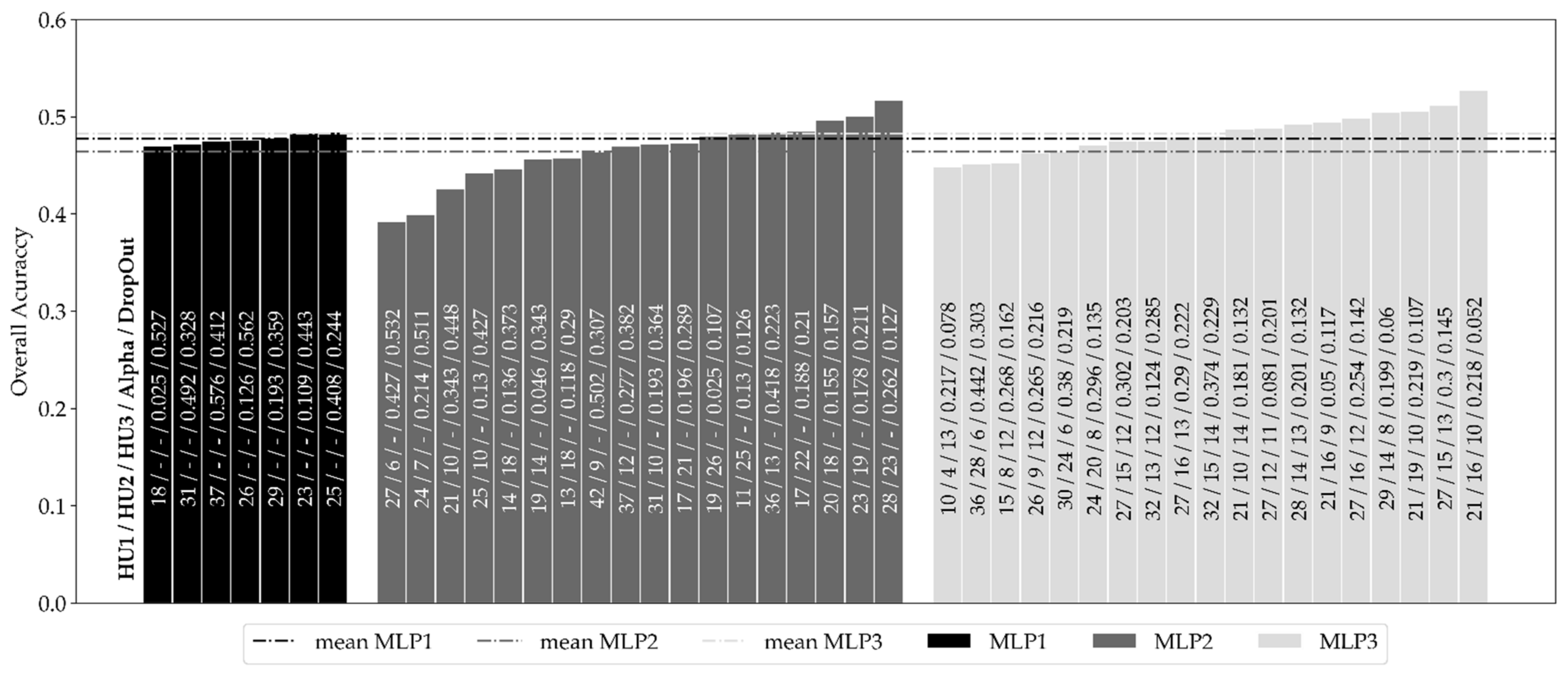
4.2.1. MLP Hyper-Parameter Optimization

As the proposed approach has a loss function which computes the L1-distance between semantic segmentations of the real and synthetic images, it was required to train the MLP net used to perform the semantic segmentation. Due to the MLP net having a key role in the quality of the proposed approach, a hyper-parameter optimization was performed, as depicted in Figure 1b.

As one of study objectives was to evaluate the generalization ability of the models to produce cloud-free images despite being trained in other images, four MSI/Sentinel-2 images were selected to perform the MLP optimization; this way, the MLP model would not be specific for just one image date. Almost-cloud-free images spread along the year were selected as shown in

Table 1. Image dates used and parameters optimized in the MLP network training.

MSI/Sentinel-2 Images	Parameters	Values
29 July 2017 22 October 2017	hidden layers	1	2	3
	hidden units	9–51	4–31	4–16
17 February 2018 10 May 2018	alpha	0–0.6
	dropout	0–0.6

. The training fields in Figure 2 were split into MLP training fields (70%) and MLP testing fields (30%) using the stratified random sampling tool available in the QGIS software. The pixels available in the MLP training fields were split into new sets, the MLP training set (70%) and the MLP validation set (30%). The training pixels were balanced replicating the pixels for the classes with fewer samples than the most popular class.

The MLP hyper-parameter optimization was carried out with the Particle Swarm Optimization (PSO) algorithm [29], due to its capacity to deal with a large space of parameters and ability to find a near-optimum solution efficiently [37]. The tuned parameters were the number of hidden layers, hidden units (neurons), the dropout value and the alpha value in the LeakyReLU loss function; the values range used to tune these parameters are presented in Table 1. The PSO implementation available in the Python package Optunity was used [38]. The MLP optimization was carried out using the PSO algorithm with 10 particles and 5 generations. Each training was performed with a batch size of 16,384, 1000 epochs and early stop with a requirement of 0.001 minimum improvement in the loss up to 60 epochs after the best model.

4.2.2. Evaluation of the MLP Custom Loss Function

The experiment to evaluate whether the MLP custom loss function provides synthetic pixels capable of improving the further semantic segmentation, was performed, as depicted in Figure 1c. Five different sets of weights (

Table 2. Different sets of weights used to evaluate the original pix2pix and the pix2pix cGAN with the MLP loss function.

Weigh Sets	A	B	C	D	E
${\lambda }_{cGAN}$	1	1	1	1	1
${\lambda }_{L1}$	100	100	100	100	100
${\lambda }_{MLP}$	0	100	200	300	400

) in the loss function components were evaluated. Set A represents the original pix2pix cGAN, while sets B–E are the proposed approach changing just the weight for the additional component (${\lambda }_{MLP}$). For that, five nets using these different sets of weights each were trained from the image group I depicted in

Table 3. Image date for the conditional and objective images.

Image Group	Month	$\mathbf{Conditional} \mathbf{Images} \left(\mathit{u}\right)$		$\mathbf{Objective} \mathbf{Image} \left(\mathit{y}\right)$
		MSI Sentinel-2	C-SAR Sentinel-1	MSI Sentinel-2
	Training images
I	June	4 June 2017	24 June 2017	24 June 2017
II	September	12 September 2017	4 September 2017	7 September 2017
III	December	1 December 2017	9 December 2017	6 December 2017
		22 October 2017
IV	March	1 March 2018	3 March 2018	6 March 2018
		14 February 2018
V	June	14 June 2018	19 June 2018	19 June 2018
	Generalization testing images
1	October	17 October 2017	10 October 2017	22 October 2017
2	April	10 May 2018	2 May 2018	30 April 2018

. The five models (A–E) as well as the conditional patches of image group I were used to generate cloud-free patches for the whole image I. Further, these patches were used to generate the synthetic images (I-A, I-B, I-C, I-D, and I-E) using just the centre part (32 × 32 pixels) of each synthetic patch.

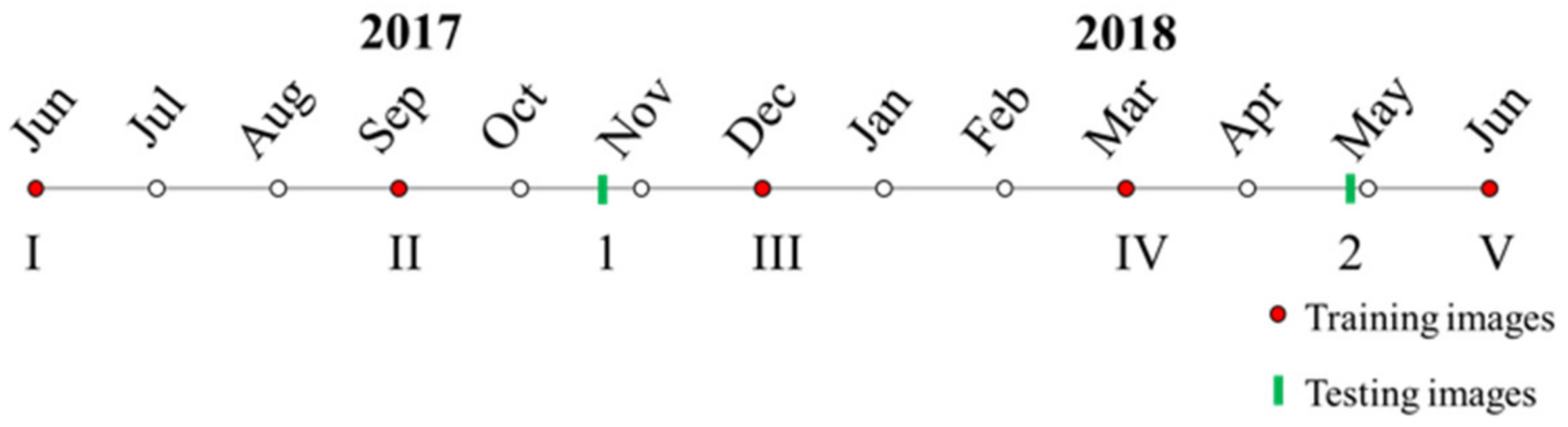
4.2.3. Evaluation of the Generative Models Generalization

The evaluation of the generative models generalization ability was carried out as shown in Figure 1d. The models were trained using different sets of images selected along the time series dataset; in the sequence, these models were applied to generated synthetic images for previously unseen images by the model. To perform the training of the models, first, five optical images were selected for every three months starting on June 2017. These images were the objective images ($y$), selected taking into account the images with less cloud and cloud shadows in the pre-chosen months (June 2017, September 2017, December 2017, March 2018 and June 2018). For each objective image, a pair (SAR and optical) as conditional images ($u$) was selected, so they were used as constraints in the cGAN. The authors tried to obtain the SAR images from the same day of each objective image. Regarding the optical conditional images, it was preferred for each objective image that the previous image available in the dataset had as low noise as possible; if it was not possible to find a suitable previous image, an image forward in the time series was selected instead. For December 2017 and March 2018, there did not exist images without clouds or with a low amount of clouds; in these cases, two optical images were selected as condition for the objective image, meaning that for some regions, one optical image was used as condition, and in other regions, another optical image was used. The image groups with the dates for the conditional and objective images selected to perform the training as well as the testing of these models are depicted in Table 3; the timeline with the temporal distribution showing where these images lie along the time series is presented in Figure 3.

The patches extracted over the training image groups depicted in Table 3 were combined into seven sets (I-II; II-III; III-IV; IV-V; I-II-III; III-IV-V; I-II-III-IV-V). These sets were created aiming to train models which could temporally embrace all images of the time series. The patches were used to train four models with two dates (I-II, II-III, III-IV and IV-V), two models with three dates (I-II-III and III-IV-V), and one model with five dates (I-II-III-IV-V). Two models were also trained using just patches extracted from the training fields (Figure 2) in testing images groups 1 and 2, also depicted in Table 3. Finally, the transfer learning (TL) approach was used to train two additional models; the model I-II-III-IV-V was chosen and was trained for 15 epochs more using patches gathered in the training fields (Figure 2) of image group 1 and image group 2 depicted in Table 3 as generalization testing images. Taking into account where images 1 and 2 temporally lie along the time series, specific models were used to create synthetic cloud-free images 1 and 2. Using the models (II-III, I-II-III, I-II-III-IV-V, I-II-III-IV-V + TL and 1) and the conditional patches of image group 1, cloud-free patches were generated for the whole image 1; further, these patches were used to generate the synthetic images (1/II-III, 1/I-II-III, 1/I-II-III-IV-V, 1/I-II-III-IV-V + TL and 1/1) using just the centre part (32 × 32 pixels) of each synthetic patch. The same was performed for image group 2, but now using the models (IV-V, III-IV-V, I-II-III-IV-V, I-II-III-IV-V + TL and 2) which were used to generate the synthetic images (2/IV-V, 2/III-IV-V, 2/I-II-III-IV-V, 2/I-II-III-IV-V + TL and 2/2). The models trained as well as the labels for the synthetic images generated with these models can be seen in

Table 4. Generative models and synthetic images used to evaluate the models generalization.

	Generative Models	Synthetic Images Labels
two images	I-II	-
	II-III	1/II-III
	III-IV	-
	IV-V	2/IV-V
three images	I-II-III	1/I-II-III
	III-IV-V	2/III-IV-V
five images	I-II-III-IV-V	1/I-II-III-IV-V
		2/I-II-III-IV-V
transfer learning	I-II-III-IV-V + TL 1	1/I-II-III-IV-V + TL 1
	I-II-III-IV-V + TL 2	2/I-II-III-IV-V + TL 2
same image	1	1/1
	2	2/2

.

In both evaluations (generative models generalization and the addition of the MLP custom loss function) the networks were trained for 200 epochs, with a batch size of eight, using the Adam version of stochastic gradient descent as optimizer with learning rate of 0.0002 and momentum of 0.5. GAN are hard to train, and it lacks a metric related to the training quality, which makes it difficult to evaluate the training progress or compare different models. To avoid issues like not achieving Nash equilibrium or mode collapse, the training process was followed using the loss for the generator and the discriminator, as well as partial results (synthetic patches). Every 10 epochs, a small number of patches were randomly selected and the generative model was applied to generated synthetic images, which were compared with their real versions. To perform the classification with the MLP added to the custom loss function, just the central part (16 × 16 pixels) of the patches was used. Although the patches had been balanced considering the central pixel, the most popular class inside a patch of 256 × 256 pixel could be different from the class of the central pixel; hence, the loss using the whole patch would take into account mainly this class and not the class of the central pixel which was aimed to constrain the pixel values.

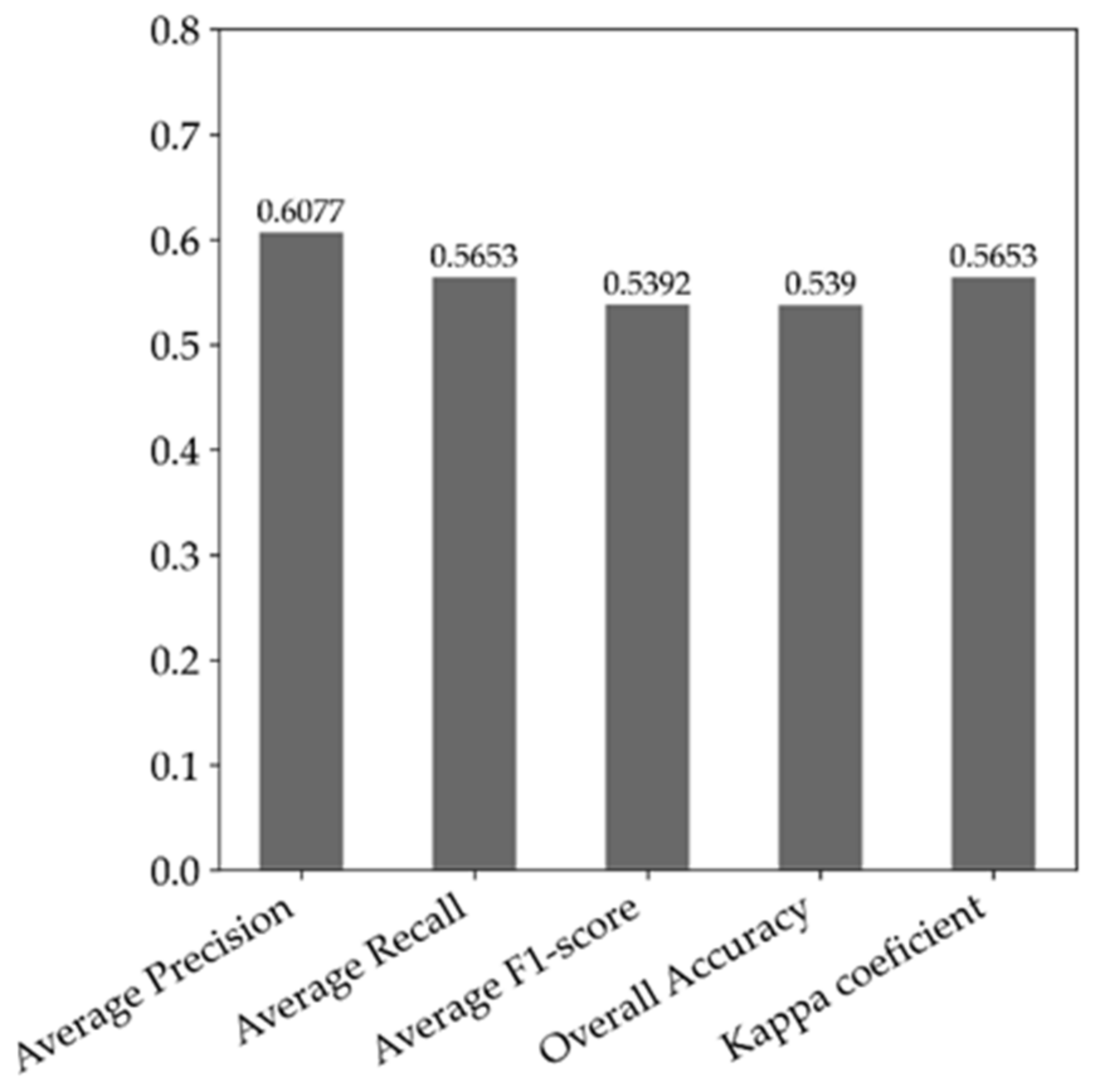
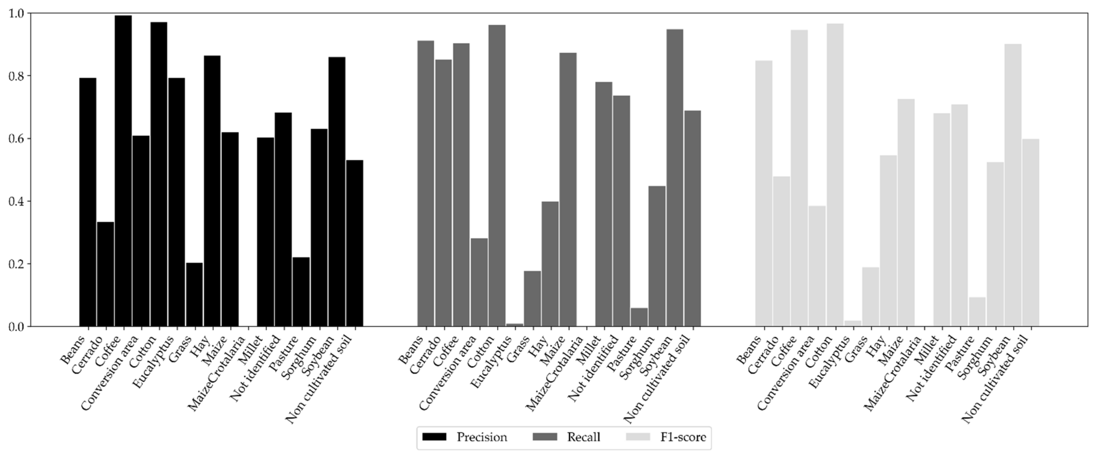
4.3. Performance Assessment

To evaluate the MLP hyper-parameter optimization and select the best MLP, the overall accuracy achieved in the validation dataset for all MLP nets trained was used; afterward, the best model considering the kappa coefficient, precision, recall and F1-score were evaluated, but now classifying the MLP testing fields created as describe in Section 4.2.1.

To assess the results regarding the additional component in the loss function (Equation (9)), a visual analysis was performed over patches randomly selected in the testing fields depicted in Figure 2. It was also compared the spectral response between the real and synthetic pixels for each model trained (A–E; Table 2), and for each crop type taking into account just the testing fields (Figure 2) and the image group I (Table 3). These images were in the sequence applied to a semantic segmentation with the random forest algorithm [39] with 2000 trees and depth equal to 12. The Python scikit-learn package [36] was used for that. The training samples were taken from the real image over the training fields presented in Figure 2. They were balanced, replicating the less popular classes. The random forest model was then applied to classify the pixels in the real image and the synthetic images (A–E; Table 2). The results were evaluated in the testing fields shown in Figure 2. The semantic segmentation results were assessed with the overall accuracy, kappa coefficient and F1-score as well as considering the F1-score for each class. To verify if the difference in the semantic segmentation results were statistically significant, McNemar’s test was used [40]. The peak-to-signal noise ratio (PSNR) as well as the structural similarity index measure (SSIM) were used to assess quantitatively the similarity between the real and synthetic images.

The model generalization capability was assessed through the quality evaluation of the sematic segmentation for the synthetic images and compared with the semantic segmentation of the real images. Using the real objective images 1 and 2 (Table 3), one random forest model for each one was trained; with these models, semantic segmentation of all synthetic images 1 (1/II-III, 1/I-II-III, 1/I-II-III-IV-V, 1/I-II-III-IV-V + TL and 1/1) and 2 (2/IV- V, 2/III- IV- V, 2/I-II-III-IV-V, 2/I-II-III-IV-V+TL and 2/2) was performed. Then, the generalization capability for these generative models was assessed using the average F1-score for these sematic segmentations considering the pixels located only over the testing fields (Figure 2).

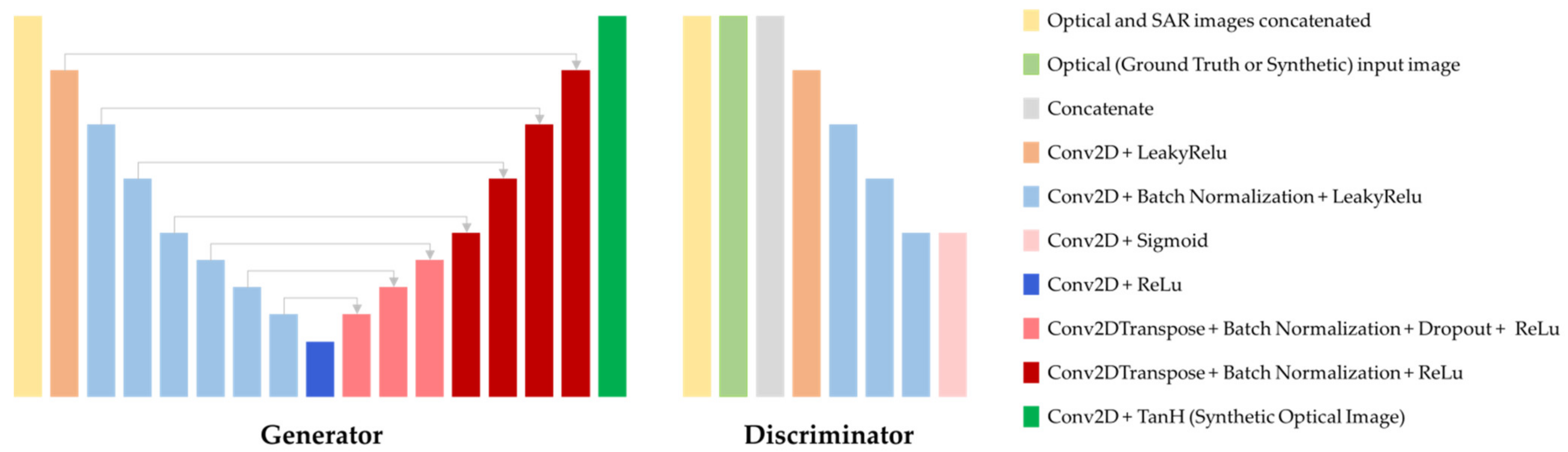
4.4. Pix2pix cGAN Architecture

The pix2pix cGAN architecture is depicted in Figure 4, where the operations in each layer are indicated in the legend. The generator had as input the conditional images (SAR and optical) patches concatenated, while its output was the synthetic cloud-free optical image patch. The discriminator had the same input as the generator plus the synthetic or real optical image patches, and its output was a matrix which indicates the probability of the optical image patch presented be real or fake. All convolutions had the spatial filter size as 5 and stride amount equal to 2. In the layers with LeakyReLu as activation function, the alpha value was 0.2, while in the layers with dropout operation the value 0.5 was selected.

5. Results

5.1. Performance of the MLP Network Models

The hyper-parameter optimization was carried out by training different MLP networks and aiming to find the best set of parameters. This process took 126.83 h (5.28 days) using a machine with Intel Xeon Silver 4110, 2.1 GHz clock, 376GB RAM and NVDIA GeForce GTX 1080Ti GPU. Depicted in Figure 5 are the overall accuracies for all MLP networks trained during the hyper-parameter optimization, the values for the parameters used in the training of each network, and the mean accuracies for the networks trained with same number of hidden layers.

The vertical lines in Figure 5 represent the overall accuracy mean value for the MLP1, MLP2 and MLP3 networks groups. In general, the networks with three hidden layers had a slightly better result than networks with just one hidden layer, and both were better than the networks trained with two hidden layers when considering the poorest results. The PSO algorithm had trained fewer networks with one hidden layer when compared with the networks trained with two and three hidden layers, and if considering just for the seven (number of networks trained with one hidden layer) best networks of each group, it possible to see that for the MLP networks with three and two hidden layers had better results than the networks with just one hidden layer. Regarding the number of hidden units in each layer and the values for the alpha in the LeakyReLU, there was not a clear pattern that can be related to the accuracy of the MLP network, whereas it seems that the accuracy of the MLP decreased when the dropout values increased, as for most of the MLP2 and MLP1 the worst results have higher values for the dropout. However, this is not a rule since for different sets of parameters it is also possible to notice higher overall accuracy values for networks with higher dropout values than others; even so, this can be related to other parameters as they were also changed.

Regarding the best set of parameters, it was selected the one which provided the higher overall accuracy during the optimization. The best set of results were obtained with three hidden layers; 21, 16 and 10 hidden units in the hidden layers one, two and three, respectively; the alpha value of 0.218; and the dropout value of 0.052. Evaluation metrics of the MLP network with the best set of parameters are depicted in Figure 6.

The overall accuracy was 0.539. The Kappa coefficient was 0.565 and can be considered as a more representative indicator than the overall accuracy, since it also takes into account the wrongly classified samples. The average Precision, Recall and F1-score were 0.607, 0.565 and 0.539, respectively.

Presented in Figure 7 are the precision, recall and F1-score for each of the 16 crop types in the testing MLP dataset; for three of the crop types there did not exist enough polygon fields in the dataset to be able to split them into training and testing data, so they were used just for training. The precision points out the commission of pixels in the class being evaluated, while the recall indicates the omission of pixels for the same class. The results in Figure 7 show that the precision was the best for coffee with 0.99, followed by cotton with 0.97, hay and soybean both with 0.86, and beans with 0.70. In general, this means that these classes had a spectral behaviour that the MLP model was capable to distinguish from other classes. The three worst classes were maize + crotalaria, grass and cerrado, which had precisions of 0.0, 0.22 and 0.33, respectively. This means that the MLP model included misclassified pixels in these classes.

Regarding the recall, the best value was 0.96 for cotton, which was followed by soybean, beans and coffee with recall of 0.94, 0.91 and 0.90, respectively. Classes maize with 0.87, cerrado with 0.85, millet with 0.78 and not-identified with 0.73 also showed high recall values considering the complexity of the problem. The high value of recall for these classes implies that the MLP model was able to classify the pixels belonging to these classes correctly with only a few pixels mislabelled in other classes. Despite most of the classes having high values for the recall, maize + crotalaria, eucalyptus and pasture presented low recall values of 0.0, 0.01 and 0.06, respectively, indicating that the MLP model was not able to label the pixels belonging to these classes correctly. The F1-score is the harmonic mean between precision and recall; hence, it indicates how well the model classifies each class. The results of F1-score were consistent with the recall results.

In summary, the best MLP model could classify well or reasonably well most of the classes, taking into account the complexity of the problem, as the classes have similar spectral behaviour, and the same crop type in images taken on different dates can have distinct spectral responses. The classes for which the model had the worst performance were in general with only few data samples, meaning a low representativeness in the dataset. Therefore, the use of the best MLP model in the custom loss function may contribute to improving the synthetic values for most of the classes and not be a serious problem for other classes, since they represented the minority in the dataset.

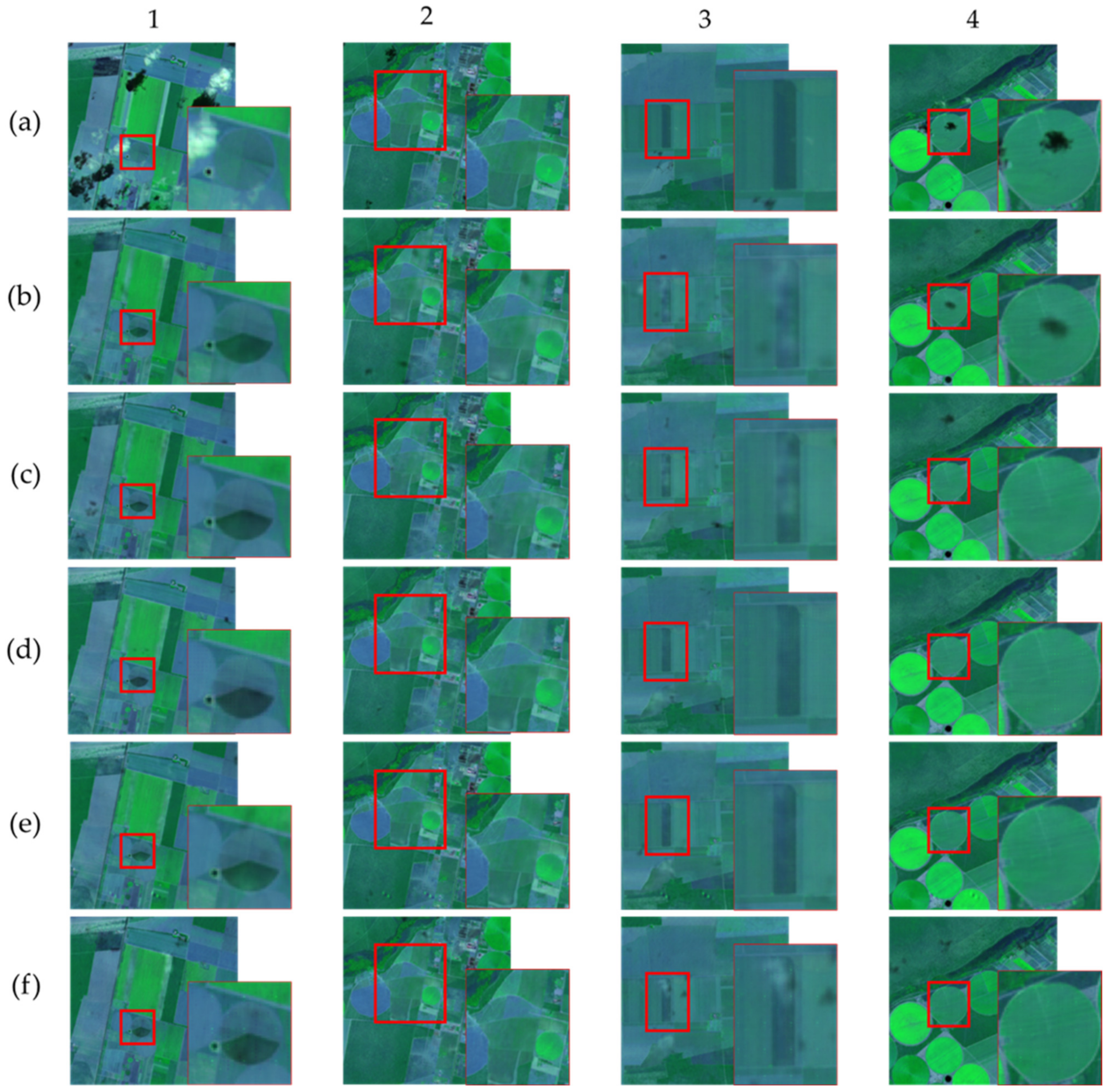
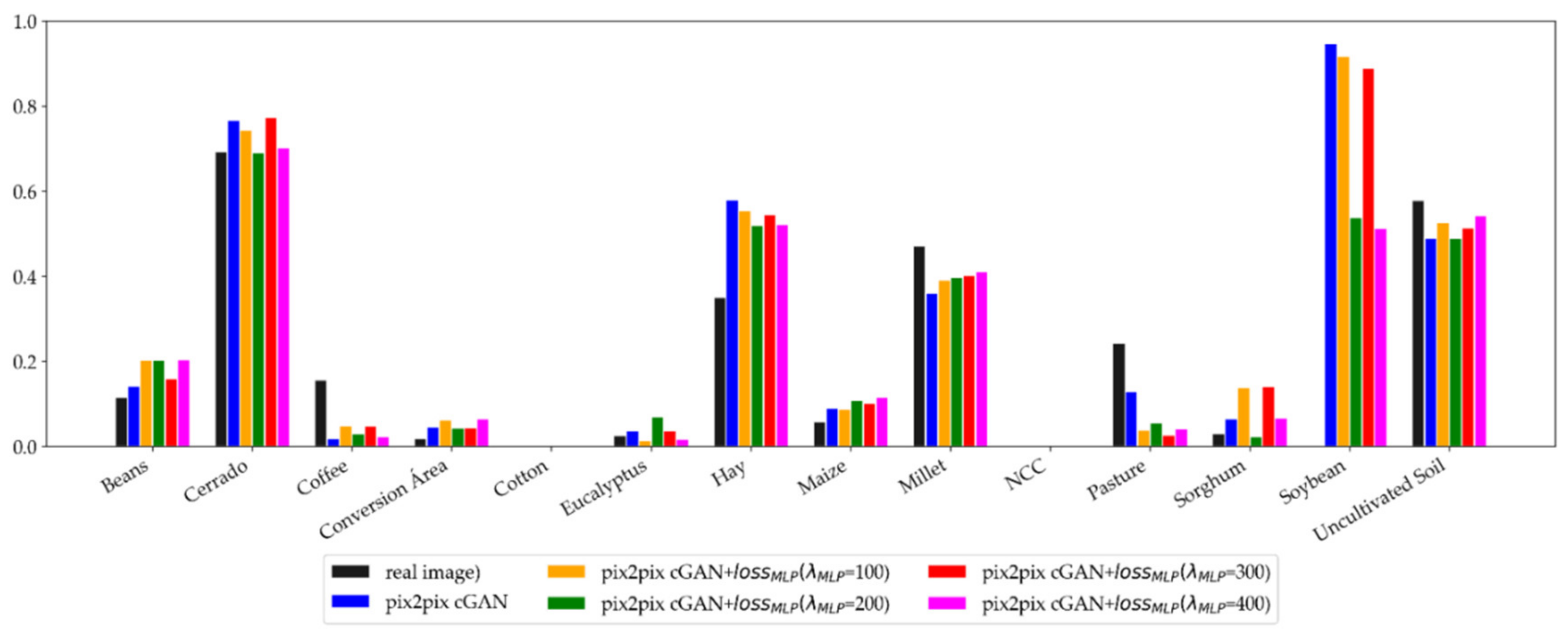
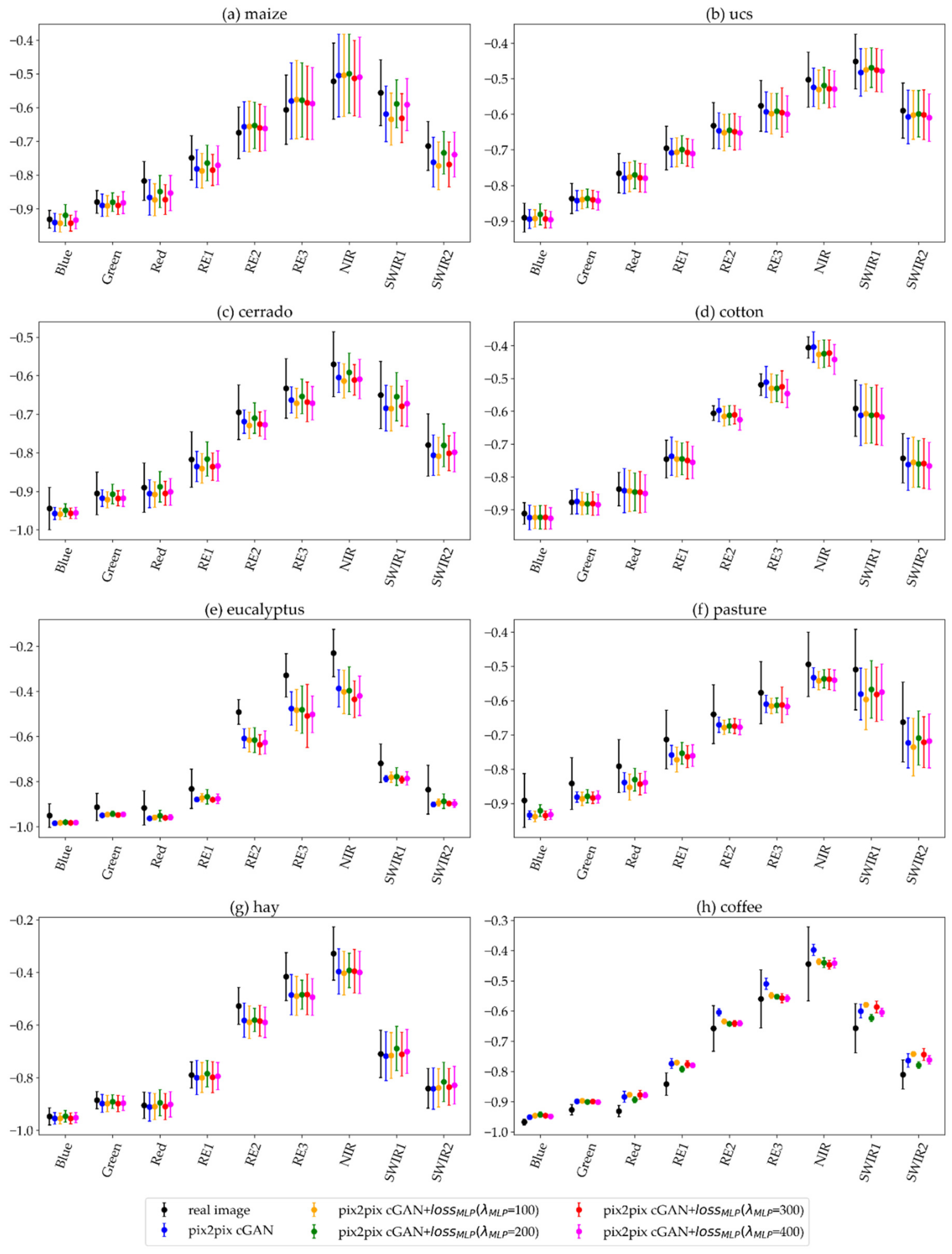
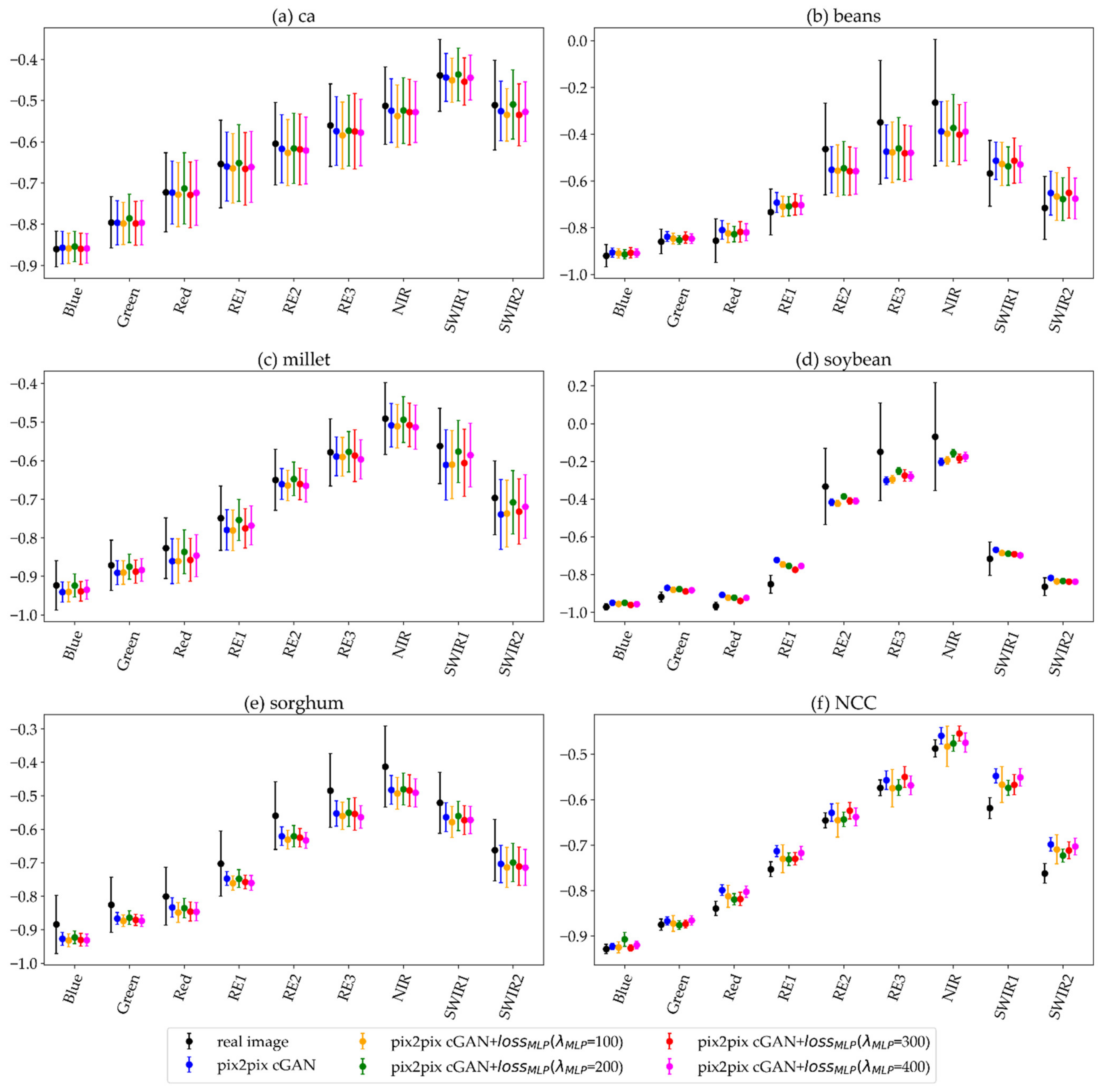
5.2. Synthetic Images Generated with the Pix2pix cGAN with the MLP Loss Function

The different methods for synthetic image generation (A–E, Table 2) were assessed using the training image group I (Table 3). Depicted in Figure 8 are patches collected over four different regions in the testing fields (Figure 2). Each row represents images generated by the same model; the patches in row (a) were collected from the real image, the patches in row (b) were generated with the original pix2pix cGAN, and the patches in rows (c), (d), (e) and (f) were generated with pix2pix cGAN with the MLP custom loss function, with varying ${\lambda }_{MLP}$ of 100, 200, 300 and 400, respectively.

Inspecting the image patches, it is possible to notice that all methods were able to generate plausible images, removing most of the clouds and cloud shadows existent in the ground truth, as can be seen mainly in rows (b–f) of column 1. However, there still exists small noises like thin clouds and small black dots appearing to be shadows in some patches; this effect is particularly more evident in patches 1(b), 2(b), 3(b) and 4(b) generated with the original pix2pix cGAN, and they also appear in patches 1(c), 3(c), 4(c) generated with the proposed approach with ${\lambda }_{MLP}$ equal to 100, as well as in patch 3(f) generated with ${\lambda }_{MLP}$ of 400. The existence of these noises seems to be unrelated to any approach, since they appear in most of the rows, and they may be related to the fact that small thresholds of cloud and cloud shadows were accepted in the training image patches (Section 4.1). Nonetheless, it is possible to see that these noises are small, and in most cases they are hardly noticeable. In the patches in rows (d) and (f), it is possible to see some salt and pepper noises, which are more clearly visible in the snippets highlighted in patches 3(d), 3(f), 4(d) and 4(f), which were generated with the proposed approach with ${\lambda }_{MLP}$ of 200 for row (d) and ${\lambda }_{MLP}$ of 400 for row (f). In row (e), generated with the proposed approach with ${\lambda }_{MLP}$ equal to 300, it is also possible to see blurred pixels which seem to be a pattern at the bottom of all patches of this row. Based on the visual analysis, it was not possible to see significant color differences between the real and the synthetic images mentioned in related articles [20,21,26]; even the original pix2pix cGAN generated plausible images with small differences among them. This may likely be related to the optical image used as condition for the pix2pix cGAN, which was selected to be as close as possible to the image desired to be generated and not from the previous year as was used by Bermudez et al. [24]. This may also be the reason for some land cover differences which happened in the same way between the real and the synthetic images for the snippets highlighted in column 1. Looking closely at the snippets highlighted in column 2, it is also possible to see that the image quality improves slightly as the ${\lambda }_{MLP}$ increases; the same appears in column 3, excluding patch 3(f). In column 4, it is possible to notice in the snippets highlighted that the pix2pix cGAN was not able to totally remove the dark shadow, while the proposed approach removed independent of the ${\lambda }_{MLP}$ used.

In general, it is possible to see that, independent of the approach or weight used, the generated synthetic pixels were very similar to the real pixels, even though there are small differences in the crop type semantic segmentation, as can be seen in

Table 5. Metrics for evaluation for the semantic segmentation and similarity between the real and synthetic images generated using different methods.

	OA	$\mathsf{\Delta }\mathit{O}\mathit{A} *$	Kappa	$\mathsf{\Delta }\mathit{K} *$	F1-Score	$\mathsf{\Delta }\mathit{F}1 *$	PSNR	SSIM
Real image	0.431	-	0.308	-	0.447	-	-	-
I-A (pix2pix cGAN)	0.414	−1.7%	0.292	−1.6%	0.425	−2.1%	22.89	0.765
$\mathrm{I}-\mathrm{B} (\mathrm{pix}2\mathrm{pix} \mathrm{cGAN}+{\lambda }_{MLP}$=100)	0.428	−0.3%	0.303	−0.5%	0.438	−0.9%	22.90	0.767
$\mathrm{I}-\mathrm{C} (\mathrm{pix}2\mathrm{pix} \mathrm{cGAN}+{\lambda }_{MLP}$=200)	0.400	−3.1%	0.269	−3.9%	0.411	−3.5%	23.16	0.777
$\mathrm{I}-\mathrm{D}(\mathrm{pix}2\mathrm{pix} \mathrm{cGAN}+{\lambda }_{MLP}$=300)	0.437	0.6%	0.313	0.6%	0.442	−0.5%	22.87	0.765
$\mathrm{I}-\mathrm{E} (\mathrm{pix}2\mathrm{pix} \mathrm{cGAN}+{\lambda }_{MLP}$= 400)	0.427	−0.4%	0.298	−1.0%	0.436	−1.0%	23.00	0.771

* Difference for Overall accuracy, Kappa coefficient and F1-score between the real image and the synthetic images in percentage.

and Figure 9.

The sematic segmentation for most of the synthetic images were close to the kappa coefficient and F1-score achieved using the real image, which were 0.308 and 0.447, respectively (Table 5). The proposed approach with ${\lambda }_{MLP}$ of 300 (I-D) provided the best results; the kappa coefficient of 0.313 was 0.6% higher than for the classification with the real image, however, the F1-score of 0.443 was 0.5% lower than for the real image. The original pix2pix cGAN (I-A) provided a kappa coefficient and the F1-score equal to 0.292 and 0.425. In general, the proposed approach provided slightly better results than the original pix2pix cGAN (I-A), except when ${\lambda }_{MLP}$ was equal to 200 (I-C), which had the worst performance. Regarding the similarity metrics PSNR and SSIM computed between the real and synthetic images, it is possible to notice that they were similar for all methods. Even so, it is possible to see that for both PSNR and SSIM, the approach with the custom loss function had a minor advantage over the original pix2pix cGAN (I-A), except when ${\lambda }_{MLP}$ was equal to 300 (I-D). However, the similarity metrics had similar values and therefore cannot be used in comparing the methods.

The McNemar’s test was used to identify if the results of different approaches were significantly different considering a significance level of 0.05. The statistics computed for each pair of semantic segmentation are depicted in

Table 6. McNemar’s test computed in paired results of all semantic segmentations performed.

	p-Value
	Real Image	A	B	C	D
Real image	-	-	-	-	-
A	$1.6 \times {10}^{-29}$	-	-	-	-
B	$4.2 \times {10}^{-3}$	$2.1 \times {10}^{-47}$	-	-	-
C	$7.7 \times {10}^{-170}$	$3.7 \times {10}^{-49}$	$5.0 \times {10}^{-182}$	-	-
D	$3.8 \times {10}^{-6}$	$8.1 \times {10}^{-140}$	$2.1 \times {10}^{-130}$	$0$	-
E	$6.3 \times {10}^{-4}$	$4.9 \times {10}^{-37}$	$0.67$	$1.2 \times {10}^{-199}$	$4.4 \times {10}^{-25}$

A: original pix2pix cGAN; B–E: pix2pix cGAN + MLP loss function with ${\lambda }_{MLP}$ equal to 100, 200, 300 and 400 respectively.

, where the values less than 0.05 indicate significant differences in the segmentation results. The p-value computed between the results of the synthetic images generated with the proposed approach with ${\lambda }_{MLP}$ of 100 (I-B) and ${\lambda }_{MLP}$ of 400 (I-E) was higher than 0.05, indicating that the results from these two models did not differ significantly. The other paired comparisons provided values smaller than 0.05, indicating significant differences.

The metrics presented above are outcomes for all crop types in the semantic segmentation, and as previously mentioned, most of the bands and crop types in the synthetic images had similar values to the real image. The spectral analysis for each crop type is presented in Figure 10 and Figure 11, considering the mean and standard deviation of the normalized surface reflectance for each band. The colors depict the processing of the image: the black color depicts the real image, the blue color the image generated with the original pix2pix cGAN, while the yellow, green, red, and pink colors depict the proposed approach with ${\lambda }_{MLP}$ of 100, 200, 300 and 400, respectively (A–E, Table 2).

The classes uncultivated soil, cerrado, cotton, conversion area and beans had pixels values very similar for the synthetic images and real image independent of the method used, while the synthetic pixel values for the classes eucalyptus, coffee and soybean were the most different.

The spectral behaviour for the class cerrado (Brazilian savannah) is depicted in Figure 10c. The mean value for most of the bands for all synthetic images had large variation; however, the standard deviation lay inside the same range as the real image. The proposed approach with ${\lambda }_{MLP}$ equal to 200 (I-C) provided the closest value to the real image; the F1-score for this image was the lowest, around 0.7, but almost the same value was obtained with the real image (Figure 9). Other tested methods had higher F1-score than the real image, e.g., the proposed approach with ${\lambda }_{MLP}$ equal to 300 (I-D) and the original cGAN (I-A) achieved F1-score values close to 0.8.

Likewise, the synthetic pixels for the class beans (Figure 11b) presented a good similarity with the real pixels. The similarity was better for the bands in the visible spectral range; for other bands, the mean values differed more from the reference, but the standard deviations were in the same range as in the real image. Regarding the classification, it is possible to see in Figure 9 that the proposed approach with ${\lambda }_{MLP}$ equal to 100 (I-B), 200 (I-C) and 400 (I-E) presented the best F1-score values, although they were around 0.2, while the ground truth achieved a lower F1-score, around 0.1.

However, the class eucalyptus (Figure 10e) had values for all bands in the synthetic images differing from the real image, with the biggest differences for the bands NIR, red-edge 2 and 3. Hence, the eucalyptus class was poorly classified, as can be seen in Figure 9; the F1-score shows the synthetic image generated with the proposed approach with ${\lambda }_{MLP}$ equal to 200 (I-C) with the best performance, which was followed closely by the proposed approach with ${\lambda }_{MLP}$ equal to 300 (I-D) and the original cGAN (I-A) having almost the same F1-score than the real image.

For most of other classes, the synthetic and real images had similar values, mainly in bands blue, green, red, while some differences can be seen in other bands for some classes. In most of the bands, the mean and standard deviation for the synthetic images generated with the proposed approach (I-B; I-C; I-D; and I-E) had a spectral response closer to the real image in comparison to the original pix2pix cGAN (I-A). This is also reflected in the F1-score, in which some of the synthetic images produced with the proposed approach had values slightly higher than the original pix2pix cGAN; even so, this approach also provided an F1-score similar to the real image.

5.3. Generalization Capability for the Pix2pix cGAN with the MLP Loss Function

The F1-scores for the sematic segmentation with the testing images (images 1 and 2) are given in Figure 12; the models were trained using different sets of the real images (1 and 2) and the synthetic images as explained in Section 4.2.3. The synthetic images were generated using the proposed approach with ${\lambda }_{MLP}$ of 300, which provided slightly better semantic segmentation results and produced synthetic pixels closer to the pixels of the real images than those produced by other methods.

The results in Figure 12 show that the sematic segmentation model trained with the real image provided an F1-score around 0.9 for image 1. Almost as good semantic segmentation results were obtained with the model trained using the synthetic images that were generated using the model trained with image 1 as well as with the model trained using the image group I-II-III-IV-V and enhanced with transfer learning for 15 epochs for image 1. The semantic segmentation performance in the synthetic image trained using image 2 was close to the performance of the semantic segmentation with the real image, providing F1-scores of around 0.7 and 0.75, respectively. However, the transfer learning approach, where the original model was trained using image group I-II-III-IV-V and enhanced using patches of image 2 for 15 epochs, did not have a performance close to the real image.

Regarding other models for the synthetic image 1, the model trained using the image group II-III provided an F1-score around 0.7; the model trained using the group I-II-III provided an F1-score slightly higher than 0.4; and the model trained using the group I-II-III-IV-V provided an F1-score close to 0.6. For image 2, the semantic segmentation using the synthetic images generated with the models trained in image groups IV-V and I-II-III-IV-V achieved an F1-score around 0.3, while the semantic segmentation of the synthetic image generated with the model trained using the image group III-IV-V had an F1-score slightly higher than 0.2.

6. Discussion

Clouds are an issue for crop type mapping with optical satellite image time series. In this research, it was proposed to add a new custom loss function to the original pix2pix cGAN to enforce the generative model to learn how to provide synthetic pixels more similar to the real images in cloud-covered regions; it was also evaluated whether models trained on images spread along the time series would be able to perform the task of generating synthetic pixels on unseen images. A summary of the results obtained in different earlier studies and with the proposed approach in the generation of optical satellite images using GAN is presented on

Table 7. Comparison of obtained results in earlier studies, with the baseline original pix2pix cGAN and the proposed approach for the generation optical satellite images using GAN.

Article	Method	Artifacts (Training/Results)	Geometry Differences	Pixel Values Differences	Semantic Segmentation (OA)
Bermudez et al. [21]	pix2pix cGAN	no/no	some	yes	Real: ~65%~85%
					Synthetic: ~55%~75%
Bermudez et al. [24]	pix2pix cGAN *	no/no	small	some	Real: 84.6%
					Synthetic: 74.6%
Enomoto et al. [20]	cGAN	-	blurred	some	-
Li et al. [26]	$\mathrm{cGAN}+{\lambda }_{SSIM}$	-	very similar	very similar **	-
Turner et al. [28]	atrous-cGAN	no/no	very similar	small	Real: ~63%~81%
					Synthetic: 62%~80%
Ours	original pix2pix cGAN	yes/yes	very similar	small	Real: 43.1%
					Synthetic: 41.4%
Ours	$\mathrm{pix}2\mathrm{pix} \mathrm{cGAN}+{\lambda }_{MLP}$ *	yes/yes *	very similar	very similar	Real: 43.1%
					Synthetic: 40%~43.7%

* Uses multi-temporal approach; ** Except for arable land.

. The results were compared considering the real and synthetic images. For that, it was compared the presence of artifacts in the training data and in the synthetic images, the existence of geometry differences, the existence of pixel values differences, as well as the semantic segmentation results.

The synthetic patches generated with the pix2pix cGAN with the MLP loss function (Figure 8) were geometrically and spectrally similar to the real patches. However, they are not perfect, as it was possible to notice the presence of small noises and artifacts, like thin clouds and small black dots appearing to be small shadows. Such artifacts were not observed in other cloud removal studies such as in Bermudez et al. [21,24], which had ideal training data. However, while these studies showed their results in areas totally cloud-free, just simulating cloud-covered areas, in this study it was chosen to use almost-cloud-free images for training and testing the generative models. Furthermore, the results showed that when using non-optimal training data (with minor clouds and cloud shadows), the proposed method outperformed the original pix2pix.

Considering the materials used, Bermudez et al. [21] addressed the process reconstructing the missing information using the pix2pix cGAN to translate Sentinel-1 into Landsat-8 images, while Bermudez et al. [24] used the pix2pix cGAN with a new multitemporal constraint. The multitemporal approach consisted in synthesizing a Landsat-8 image, using as condition a Sentinel-1 image acquired as close as possible to the image to be generated, plus Sentinel-1 and Landsat-8 images collected in the same month but one year early. Other studies addressed the reconstruction of optical images also through image translation. Enomoto et al. [20] translated SAR/ALOS-PALSAR images to red, green and NIR Terra-ASTER images using cGAN. Li et al. [26] used pix2pix cGAN with a structural similarity index measure (SSIM) as a new term in the pix2pix cGAN objective function. Turnes et al. [28] presented the atrous-cGAN to perform SAR to optical image translation. Despite their overall success regarding the geometry in the synthetic images, most of them highlight some issues. In Enomoto et al. [20], fine objects were blurred and synthetic pixel values were quite different from real pixels. In Bermudez et al. [21], it was possible to see geometric and spectral differences between the synthetic and real images. Similar to Bermudez et al. [24], this study followed the multitemporal approach; however, the authors chose to use just one Sentinel-1 image and one Sentinel-2 image as conditional data. Another difference was that it was used an optical image acquired as close as possible to the image to be generated. The synthetic patches in Li et al. [26] presented a high geometric and spectral similarity with real patches most of the land cover types; however, their approach had problems in arable land areas, as different crop types have different spectral response which were not totally sensed by the backscattering coefficients on the SAR images. Despite different datasets, comparing the synthetic crop patches presented in this study with patches showed in the Bermudez et al. [21,24] and Li et al. [26] with their respective real image patches, it is possible to notice that the temporal constraint with the optical image acquired close to the image to be generated as well as using the MLP loss function, improves the pixel values similarity.

Regarding the semantic segmentation, similar values were achieved for the F1-score and kappa coefficient for the synthetic image and real images, while Bermudez et al. [21,24], who also performed crop type semantic segmentation using the random forest algorithm, had a significant decrease in the accuracy for the synthetic images compared to the real images. In Bermudez et al. [21], the real images had overall accuracies between 65% and 85%, while the synthetic images showed a decrease of around 20%. In Bermudez et al. [24], the F1-score in the real image was 51.4%, and the best and worst values for the synthetic images were 46.8% and 35.6%, respectively. However, in both articles, the evaluation metrics for the semantic segmentation in the synthetic images were higher than for the SAR images, showing that the SAR to optical image translation may improve further the crop type semantic segmentation. Turnes et al. [28] carried out a semantic segmentation using a U-Net presented by Ronneberger et al. [41]. Unlike aforementioned studies, they achieved close values for the F1-score and overall accuracy for synthetic and real images. The F1-score for the crop type semantic segmentation in the real image was 80% in the Campo Verde (CV) dataset and around 65% in the LEM dataset. The synthetic images generated with the atrous-cGAN presented F1-scores slightly inferior to 80% and around 60% for the same datasets. However, they classified just the most popular classes in each dataset; they grouped less popular crop types in both datasets, retaining three classes in the CV dataset and four classes in the LEM dataset. In this study, the semantic segmentation in the real image achieved an F1-score of 44.7%, while in the synthetic image generated with the original pix2pix cGAN achieved 42.5%, and the synthetic image generated pix2pix cGAN with ${\lambda }_{MLP}$ of 300 achieved 44.2%. This shows that the proposed approach delivered synthetic pixels consistent with the real pixels, and that the MLP loss function contributed to provide slightly better pixel values.

Regarding the temporal generalization, the semantic segmentation results (Figure 12) showed that the synthetic images generated with models trained in same image provided better synthetic pixels, as the F1-score for both images were similar than for the real images. However, the complication in this approach is that the image to which it is desired to perform cloud removal does not always have enough cloud-free regions to perform the training entirely on it or even for few epochs to perform the transfer learning approach. This situation is even more likely during the rainy season when many images in the time series are totally cloud-covered. Another matter regarding these approaches can be seen with image 2, where the transfer learning approach did not achieve the same results achieved in image 1. This shows that even with cloud-free patches available, the transfer learning approach will not always lead to plausible synthetic spectral pixels.

The semantic classification results for image 1 show that the synthetic images generated with models trained using image group I-II-III deliver pixels less consistent with the real image than the models trained using image groups with II-III and I-II-III-IV-V. For the model II-III, this is somewhat expected, as it should share higher similarity with image 1 than the models trained with more images. For the same reason, it was expected poorer outcome for the model I-II-III-IV-V than for the model I-II-III; however, for image 1 the model trained with five images provided a better outcome than the model trained with three images. Despite the F1-scores for the semantic segmentations for image 2 being poorer than for image 1, it is possible to see that the model trained with three images (III-IV-V) presented a worse performance than the models trained with two (IV-V) and five images (I-II-III-IV-V), similar to image 1.

7. Conclusions

This article presented two major contributions. Firstly, it was proposed to add an MLP loss function to the pix2pix cGAN objective function aiming to minimize the distance between the semantic segmentation for the real and the synthetic images during the training generative models to deliver high quality synthetic pixels to cloud-covered areas in optical images. Secondly, it was evaluated the generalization of generative models, to verify whether models trained in few images selected along the times series could able to provide plausible synthetic pixels for cloud-covered areas on unseen images along a cropland satellite image time series.

An MLP network was used to perform the semantic segmentation in the proposed loss function. Then, MLP hyper-parameter optimization was performed by training several MLP nets with different sets of parameters; the model with three hidden layers as well as with lower value for dropout provided the best accuracy values, while there were no clear patterns for other parameters that can be related to the final accuracy of the MLP. In summary, the MLP model provided a reasonable accuracy when considering the complexity of the problem and the data used. To evaluate the inclusion of the MLP loss function to the pix2pix cGAN objective function, the original pix2pix cGAN was compared with the proposed approach using different weights in the MLP loss function. Through visual comparison of the mean and standard deviation values of pixels extracted from the real and synthetic images as well as analyzing their semantic segmentation, it was possible to verify that the proposed approach provided synthetic pixels slightly better than the original cGAN, removing most of the noise that the pix2pix cGAN could not remove. Even though the pixel values for the proposed approach and the original pix2pix cGAN were close, the semantic segmentation results showed that the proposed approach may deliver more suitable pixels for crop type mapping than the original pix2pix cGAN.

Regarding the generalization, the results showed that the models trained utilizing the patches of the same image provided better synthetic pixels than the models trained utilizing patches of other images; however, the image for which the cloud removal must be performed does not always have cloud-free regions that can be used for training. The models trained with three and five images selected every three months provided poorer results for both images evaluated, and due to the computational cost, it is usually unfeasible to train more models using images selected with a higher frequency along with the time series. However, the models trained using image groups with two images selected every three months along the time series for image 1, as well as with three and five images for image 2 provided promising results, and it is possible to consider that these models can be an acceptable solution when the image is totally cloud-covered. However, further research is necessary to investigate and improve the generalization capability of generative models to perform cloud removal in cropland time series dataset.

Despite the fact that the proposed approach provided plausible synthetic pixels, there are still limitations such as small pixel value differences between the real and synthetic images, as well as the presence of very small noises appearing to be clouds and cloud shadows in the synthetic images, which were due to the artifacts in the training data. Moreover, the MLP was trained to identify crop types with images gathered in different dates, which may have affected the synthetic images, since it is well known that the same crop type can have different spectral responses on different dates. Another issue is that GAN are hard to train, and it lacks a metric related to the quality of the training, which makes it difficult to evaluate the training progress or compare different models. In future work, questions related to the GAN training can be addressed using a pix2pix Wasserstain cGAN, in which the Wasserstain distance is used as a loss measure to provide a metric which can be used to evaluate the quality of the generative model along the training, as well as to explore the metaheuristics with swarm intelligence to improve GAN training and the quality of generated images. Regarding the small noises that continue to appear in the generative images, it can likely be diminished using a more robust classifier inside the loss function, such as a U-net classifier or crop type classifier model trained in another dataset, as well as using as short sequences of SAR images as condition in the cGAN.

References

1. United Nations. Transforming our world: The 2030 Agenda for Sustainable Development. In United Nations General Assembly; United Nations: New York, NY, USA, 2015. [Google Scholar]
2. Whitcraft, A.K.; Becker-Reshef, I.; Justice, C.O.; Gifford, L.; Kavvada, A.; Jarvis, I. No pixel left behind: Toward integrating Earth Observations for agriculture into the United Nations Sustainable Development Goals framework. Remote Sens. Environ. 2019, 235, 111470. [Google Scholar] [CrossRef]
3. Karthikeyan, L.; Chawla, I.; Mishra, A.K. A review of remote sensing applications in agriculture for food security: Crop growth and yield, irrigation, and crop losses. J. Hydrol. 2020, 586, 124905. [Google Scholar] [CrossRef]
4. Atzberger, C. Advances in remote sensing of agriculture: Context description, existing operational monitoring systems and major information needs. Remote Sens. 2013, 5, 949–981. [Google Scholar] [CrossRef] [Green Version]
5. Fritz, S.; See, L.; Bayas, J.C.L.; Waldner, F.; Jacques, D.; Becker-Reshef, I.; Whitcraft, A.; Baruth, B.; Bonifacio, R.; Crutchfield, J.; et al. A comparison of global agricultural monitoring systems and current gaps. Agric. Syst. 2019, 168, 258–272. [Google Scholar] [CrossRef]
6. Whitcraft, A.K.; Becker-Reshef, I.; Killough, B.D.; Justice, C.O. Meeting earth observation requirements for global agricultural monitoring: An evaluation of the revisit capabilities of current and planned moderate resolution optical earth observing missions. Remote Sens. 2015, 7, 1482–1503. [Google Scholar] [CrossRef] [Green Version]
7. Whitcraft, A.K.; Vermote, E.F.; Becker-Reshef, I.; Justice, C.O. Cloud cover throughout the agricultural growing season: Impacts on passive optical earth observations. Remote Sens. Environ. 2015, 156, 438–447. [Google Scholar] [CrossRef]
8. King, M.D.; Platnick, S.; Menzel, W.P.; Ackerman, S.; Hubanks, P.A. Spatial and temporal distribution of clouds observed by MODIS onboard the Terra and Aqua satellites. IEEE Trans. Geosci. Remote Sens. 2013, 51, 3826–3852. [Google Scholar] [CrossRef]
9. Prudente, V.H.R.; Martins, V.S.; Vieira, D.C.; Silva, N.R.D.F.E.; Adami, M.; Sanches, I.D. Limitations of cloud cover for optical remote sensing of agricultural areas across South America. Remote Sens. Appl. Soc. Environ. 2020, 20, 100414. [Google Scholar] [CrossRef]
10. Sarukkai, V.; Jain, A.; Uzkent, B.; Ermon, S. Cloud Removal in Satellite Images Using Spatiotemporal Generative Networks. In Proceedings of the IEEE Winter Conference on Applications of Computer Vision (WACV), Snowmass, CO, USA, 1–5 March 2020; pp. 1785–1794. [Google Scholar]
11. Shen, H.; Li, X.; Cheng, Q.; Zeng, C.; Yang, G.; Li, H.; Zhang, L. Missing information reconstruction of remote sensing data: A technical review. IEEE Geosci. Remote Sens. Mag. 2015, 3, 61–85. [Google Scholar] [CrossRef]
12. Li, M.; Liew, S.C.; Kwoh, L.K. Automated production of cloud-free and cloud shadow-free image mosaics from cloudy satellite imagery. In Proceedings of the XXth ISPRS Congress, Toulouse, France, 21–25 July 2003; pp. 12–13. [Google Scholar]
13. Melgani, F. Contextual reconstruction of cloud-contaminated multitemporal multispectral images. IEEE Trans. Geosci. Remote Sens. 2006, 44, 442–455. [Google Scholar] [CrossRef]
14. Benabdelkader, S.; Melgani, F.; Boulemden, M. Cloud-contaminated image reconstruction with contextual spatio-spectral information. In Proceeding of the IGARSS 2007 IEEE International Geoscience and Remote Sensing Symposium, Barcelona, Spain, 23–28 July 2007; pp. 373–376. [Google Scholar]
15. Benabdelkader, S.; Melgani, F. Contextual spatiospectral postreconstruction of cloud-contaminated images. IEEE Geosci. Remote Sens. Lett. 2008, 5, 204–208. [Google Scholar] [CrossRef]
16. Gómez-Chova, L.; Amorós-López, J.; Mateo-García, G.; Muñoz-Marí, J.; Camps-Valls, G. Cloud masking and removal in remote sensing image time series. J. Appl. Remote Sens. 2017, 11, 015005. [Google Scholar] [CrossRef]
17. Shao, Y.; Lunetta, R.S.; Wheeler, B.; Iiames, J.S.; Campbell, J.B. An evaluation of time-series smoothing algorithms for land-cover classifications using MODIS-NDVI multi-temporal data. Remote Sens. Environ. 2016, 174, 258–265. [Google Scholar] [CrossRef]
18. Christovam, L.; Shimabukuro, M.H.; Galo, M.L.B.T.; Honkavaara, E. Evaluation of SAR to Optical Image Translation Using Conditional Generative Adversarial Network for Cloud Removal in a Crop Dataset. ISPRS Int. Arch. Photogramm. Remote Sens. Spat. Inf. Sci. 2021, 43, 823–828. [Google Scholar] [CrossRef]
19. Goodfellow, I.; Pouget-Abadie, J.; Mirza, M.; Xu, B.; Arde-Farley, D.; Ozair, S.; Courville, A.; Bengio, Y. Generative adversarial nets. Adv. Neural Inf. Processing Syst. 2014, 2, 2672–2680. [Google Scholar]
20. Enomoto, K.; Sakurada, K.; Wang, W.; Kawaguchi, N. Image translation between SAR and optical imagery with generative adversarial nets. In Proceedings of the IGARSS 2018-2018 IEEE International Geoscience and Remote Sensing Symposium, Valencia, Spain, 22–27 July 2018; pp. 1752–1755. [Google Scholar]
21. Bermudez, J.; Happ, P.N.; Oliveira, D.A.B.; Feitosa, R.Q. SAR to optical image synthesis for cloud removal with generative adversarial networks. ISPRS Ann. Photogramm. Remote Sens. ISPRS Ann. Photogramm. Remote Sens. Spat. Inf. Sci. 2018, 4, 5–11. [Google Scholar] [CrossRef] [Green Version]
22. Grohnfeldt, C.; Schmitt, M.; Zhu, X. A Conditional Generative Adversarial Network to Fuse SAR And Multispectral Optical Data For Cloud Removal From Sentinel-2 Images. In Proceedings of the IGARSS 2018—2018 IEEE International Geoscience and Remote Sensing Symposium, Valencia, Spain, 22–27 July 2018; pp. 1726–1729. [Google Scholar]
23. Singh, P.; Komodakis, N. IEEE Cloud-gan: Cloud removal for sentinel-2 imagery using a cyclic consistent generative adversarial networks. In Proceedings of the IGARSS 2018–2018 IEEE International Geoscience and Remote Sensing Symposium, Valencia, Spain, 22–27 July 2018; pp. 1772–1775. [Google Scholar]
24. Bermudez, J.D.; Happ, P.N.; Feitosa, R.Q.; Oliveira, D.A.B. Synthesis of multispectral optical images from SAR/optical multitemporal data using conditional generative adversarial networks. IEEE Geosci. Remote Sens. Lett. 2019, 16, 1220–1224. [Google Scholar] [CrossRef]
25. Sanches, I.D.A.; Feitosa, R.Q.; Diaz, P.M.A.; Soares, M.D.; Luiz, A.J.B.; Schultz, B.; Maurano, L.E.P. Campo Verde database: Seeking to improve agricultural remote sensing of tropical areas. IEEE Geosci. Remote Sens. Lett. 2018, 15, 369–373. [Google Scholar] [CrossRef]
26. Li, Y.; Fu, R.; Meng, X.; Jin, W.; Shao, F. A SAR-to-optical image translation method based on conditional generation adversarial network (cGAN). IEEE Access. 2020, 8, 60338–60343. [Google Scholar] [CrossRef]
27. Isola, P.; Zhu, J.-Y.; Zhou, T.; Efros, A. Image-to-image translation with conditional adversarial networks. In Proceedings of the IEEE Conference on Computer Vision and Pattern Recognition, Honolulu, HI, USA, 21–26 July 2017; IEEE: Piscataway, NJ, USA, 2017; pp. 1125–1134. [Google Scholar]
28. Turnes, J.N.; Castro, J.D.B.; Torres, D.L.; Vega, P.J.S.; Feitosa, R.Q.; Happ, P.N. Atrous cGAN for SAR to Optical Image Translation. IEEE Geosci. Remote Sens. Lett. 2020, 19, 3031199. [Google Scholar]
29. Lorenzo, P.R.; Nalepa, J.; Kawulok, M.; Ramos, L.S.; Pastor, J.R. Particle swarm optimization for hyper-parameter selection in deep neural networks. In Proceedings of the genetic and evolutionary computation conference, Berlin, Germany, 1 July 2017; pp. 481–488. [Google Scholar]
30. Rodríguez-de-la-Cruz, J.A.; Acosta-Mesa, H.-G.; Mezura-Montes, E. Evolution of Generative Adversarial Networks Using PSO for Synthesis of COVID-19 Chest X-ray Images, 2021 IEEE Congress on Evolutionary Computation (CEC); IEEE: Kraków, Poland, 2021; pp. 2226–2233. [Google Scholar]
31. Optimized convolutional neural network by firefly algorithm for magnetic resonance image classification of glioma brain tumor grade. J. Real-Time Image Processing 2021, 18, 1085–1098. [CrossRef]
32. Zhang, L.; Zhao, L. High-quality face image generation using particle swarm optimization-based generative adversarial networks. Future Gener. Comput. Syst. 2021, 122, 98–104. [Google Scholar] [CrossRef]
33. Mirza, M.; Osindero, S. Conditional Generative Adversarial Nets. arXiv 2014, arXiv:1411.1784. [Google Scholar]
34. Pathak, D.; Krahenbuhl, P.; Donahue, J.; Darrell, T.; Efros, A.A. Context encoders: Feature learning by inpainting. In Proceedings of the IEEE conference on computer vision and pattern recognition, Las Vegas, NV, USA, June 26–July 1 2016; pp. 2536–2544. [Google Scholar]
35. Sanches, I.; Feitosa, R.Q.; Achanccaray, P.; Montibeller, B.; Luiz, A.J.B.; Soares, M.D.; Prudente, V.H.R.; Vieira, D.C.; Maurano, L.E.P. LEM benchmark database for tropical agricultural remote sensing application. ISPRS International Archives of the Photogrammetry, Remote Sensing and Spatial Information Science; ISPRS: Karlsruhe, Germany, 2018; Volume 42, pp. 387–392. [Google Scholar]
36. Pedregosa, F.; Varoquaux, G.; Gramfort, A.; Michel, V.; Thirion, B.; Grisel, O.; Blondel, M.; Prettenhofer, P.; Weiss, R.; Dubourg, V.; et al. Scikit-learn: Machine learning in Python. J. Mach. Learn. Res. 2011, 12, 2825–2830. [Google Scholar]
37. Yang, L.; Shami, A. On hyperparameter optimization of machine learning algorithms: Theory and practice. Neurocomputing 2020, 415, 295–316. [Google Scholar] [CrossRef]
38. Claesen, M.; Simm, J.; Popovic, D.; Moreau, Y.; Moor, B.D. Easy hyperparameter search using optunity. arXiv 2014, arXiv:1412.1114. [Google Scholar]
39. Breiman, L. Random forests. Mach. Learn. 2001, 45, 5–32. [Google Scholar] [CrossRef] [Green Version]
40. Dietterich, T.G. Approximate statistical tests for comparing supervised classification learning algorithms. Neural Comput. 1998, 10, 1895–1923. [Google Scholar] [CrossRef] [Green Version]
41. Ronneberger, O.; Fischer, P.; Brox, T. U-Net: Convolutional Networks for Biomedical Image Segmentation. In Medical Image Computing and Computer-Assisted Intervention—MICCAI 2015. Lecture Notes in Computer Science, 9351; Navab, N., Hornegger, J., Wells, W., Frangi, A., Eds.; Springer: Cham, Switzerland, 2015; pp. 234–241. [Google Scholar]
Figure 1. Flowchart with the main phases carried out in the study: (a) Dataset and satellite image pre-processing; (b) MLP hyper-parameter optimization; (c) Evaluation of the MLP custom loss function; and (d) Evaluation of the generative models generalization.
Remotesensing 14 00144 g001
Figure 2. Luís Eduardo Magalhães municipality boundaries with ground truth polygons highlighting training and testing fields.
Remotesensing 14 00144 g002
Figure 3. Temporal distribution of training and testing images along the LEM dataset.
Remotesensing 14 00144 g003
Figure 4. Pix2pix cGAN architecture (Generator and Discriminator).
Remotesensing 14 00144 g004
Figure 5. Overall accuracy for all MLP networks trained during the hyper-parameter optimization. MLP1, MLP2 and MLP3 represent the number of hidden layers in the networks which could be one, two or three, respectively. The parameters values in each MLP network are presented inside each bar, where HU1, HU2, HU3 stands for Hidden Units (neurons) on layers one, two and three, respectively.
Remotesensing 14 00144 g005
Figure 6. Metrics of general evaluation for the MLP network best model: Average Precision, Average Recall and Average F1-score Overall Accuracy and Kappa Coefficient.
Remotesensing 14 00144 g006
Figure 7. Precision, recall and F1-score for each class available in the MLP testing dataset.
Remotesensing 14 00144 g007
Figure 8. Patches collected over four (14) different areas of the testing fields. Patches presented in each row were generated by the same model. Row (a) presents the patches collected on the real image, while generated patches produced with pix2pix cGAN with the MLP custom loss function with λ M L P of 0, 100, 200, 300 and 400 are presented in rows (be), and (f), respectively.
Remotesensing 14 00144 g008
Figure 9. F1-score for the semantic classification in the real and generated images.
Remotesensing 14 00144 g009
Figure 10. Pixel values comparison between the real and synthetic images produced with the original pix2pix cGAN (I-A) and the proposed approach with λMLP equal to 100 (I-B) , 200 (I-C), 300 (I-D) and 400 (I-E) for the classes: (a) maize; (b) UCS; (c) cerrado; (d) cotton; (e) eucalyptus; (f) pasture; (g) hay; and (h) coffee.
Remotesensing 14 00144 g010
Figure 11. Pixel values comparison between the real and synthetic images produced with the original pix2pix cGAN (I-A) and the proposed approach with λMLP equal to 100 (I-B), 200 (I-C), 300 (I-D) and 400 (I-E) for the classes: (a) conversion area; (b) beans; (c) millet; (d) soybean; (e) sorghum; and (f) NCC.
Remotesensing 14 00144 g011
Figure 12. F1-scores achieved in the sematic segmentation for the testing images (1 and 2) in the real and synthetic images generated with proposed approach with λ M L P = 300, but generated with models trained in different sets of images.
Remotesensing 14 00144 g012