Abstract
Satellite laser altimetry can obtain sub-meter or even centimeter-scale surface elevation data over large areas, but it is inevitably affected by scattering caused by clouds, aerosols, and other atmospheric particles. This laser ranging error caused by scattering cannot be ignored. In this study, we systematically combined existing atmospheric scattering identification technology used in satellite laser altimetry and observed that the traditional algorithm cannot effectively estimate the laser multiple scattering of the GaoFen-7 (GF-7) satellite. To solve this problem, we used data from the GF-7 satellite to analyze the importance of atmospheric scattering and propose an identification scheme for atmospheric scattering data over land and water areas. We also used a look-up table and a multi-layer perceptron (MLP) model to identify and correct atmospheric scattering, for which the availability of land and water data reached 16.67% and 26.09%, respectively. After correction using the MLP model, the availability of land and water data increased to 21% and 30%, respectively. These corrections mitigated the low identification accuracy due to atmospheric scattering, which is significant for facilitating satellite laser altimetry data processing.
1. Introduction
Satellite laser altimetry, a subclass of spaceborne Light Detection and Ranging (LiDAR), has developed into a novel Earth observation technology. It has received significant attention due to its capacity to obtain sub-meter or even centimeter-scale elevation measurement accuracies [1,2]. In 2003 and 2018, the National Aeronautics and Space Administration (NASA) launched the ice, cloud, and land elevation satellite (ICESat) and ICESat-2, which have yielded several scientific achievements regarding changes in polar ice sheet thicknesses, global tree heights, biomass inversion, global elevation control point acquisitions, and lake water level monitoring [3,4,5]. ICESat-2 is equipped with an advanced topographic laser altimeter system (ATLAS) that uses a new photon counting system. Furthermore, the number of beams and laser spot density have been improved compared to those of ICESat [6,7]. In 2018, NASA launched the Global Ecosystem Dynamics Investigation (GEDI) LiDAR system, which was successfully deployed on the International Space Station (ISS) [8]. GEDI is predominantly used to obtain surface elevations and vertical forest structures in tropical and temperate regions. In 2016, China launched the ZiYuan-3 02 satellite [9,10], which was equipped with an experimental laser altimeter, which led to subsequent satellite development. In November 2019, China launched the first sub-meter optical transmission stereo mapping satellite, GaoFen-7 (GF-7) [11,12], which was equipped with a laser altimeter to obtain elevation control points and assist with stereo mapping of double-line array images. In addition, China plans to include a multi-beam linear full-wave laser altimeter system on the terrestrial ecosystem carbon monitoring satellite to be launched in 2022.
Unlike the lunar observer laser altimeter (LOLA) and the Mars Orbiter Laser Altimeter (MOLA), laser height measurements of extraterrestrial bodies such as the Moon and Mars [13,14] differ from similar measurements conducted on the Earth. They are not only affected by the complex terrain but also by atmospheric influences on laser ranging. Therefore, the final accuracy of the height measurement must be considered for Earth observations [15,16]. During atmospheric transmission, absorption and scattering by particles such as clouds and aerosols deform the center of mass of the laser beam and range deviations [17]. However, the current atmospheric scattering correction has not been implemented commercially, leading to laser spot quality degradation due to atmospheric scattering, which reduces either the overall usability or the reliability of the precision. Exploring the effects of atmospheric scattering is a long-term process. Platt et al. [18] emphasized the influence of multiple scattering in cirrus clouds for the first time in 1981. On this basis, Mahesh et al. [19] simulated and calculated the influence of clouds on photon multiple scattering in GLAS using a Monte Carlo model [20]. Their results indicate that the path delay caused by atmospheric multiple scattering is over 20 cm for low thin clouds. However, this study is solely based on a simulation, involving the analyses of the simulation results. Brenner et al. [21] compared radar altimetry data from the Envisat and GLAS systems and observed that atmospheric multiple scattering effects comprise an important factor that affects laser ranging accuracy. Based on a semi-analytical Monte Carlo simulation, Chen et al. [22] investigated the influence of cloud multiple scattering on the accuracy of laser height measurements under specific conditions. The results indicate that the height measurement deviations depend on the cloud height, cloud effective particle radius, cloud optical thickness, concentration, and other factors. It is therefore necessary to correct height measurement deviations using real-time atmospheric observation parameters and the semi-analytical Monte Carlo method to improve the ranging values. However, it is difficult to obtain real-time atmospheric data synchronously during actual observations. Yao et al. [23] analyzed the atmospheric range waveform data from ICESat and inverted the cloud optical depth (COD) and other parameters, which provided a reference for the subsequent correction of the atmospheric scattering delay [24]. Duda et al. [25] conducted Monte Carlo simulations based on GLAS parameters and observed that clouds with a COD of 0.2 caused a height deviation of 20 cm. The 3-D Monte Carlo simulations based on ATLAS parameters conducted by Yang et al. [26] indicated that clouds with a COD of 1 will cause height deviations of 4–6 cm [27].
Previous studies have indicated that the influence of an atmospheric scattering delay cannot be ignored for high-precision laser measurements at a decimeter or centimeter scale. In this study, we first combed the atmospheric scattering identification schemes used to operate existing satellite laser altimetry systems. Then, combined with data from GF-7 laser height measurements, we analyzed the height deviations caused by atmospheric scattering. Finally, we proposed an atmospheric scattering error correction scheme according to the characteristics of the data, providing new ideas for subsequent technical developments related to laser altimetry satellites.
2. Data and Methods
The laser system of the GF-7 satellite uses a dual-beam laser that emits 1064 nm laser pulses towards the ground at a working frequency of 3 Hz and forms discrete laser spots on the ground at intervals of ~2.4 km along the orbit and at intervals of 12.25 km along the vertical orbit. As shown in Figure 1, two columns of 16 laser spots exist in the range of 20 km wide linear remote sensing images. Unlike CALIOP, which records the entire profile of data in the atmospheric transmission range to realize atmospheric detection, the GF-7 system can acquire the echo waveform from the surface to a height of 60 m. The laser scoring system onboard the GF-7 satellite is equipped with a laser footprint camera (LFC) that shares a telescope with the laser receiver and is mainly used to capture the laser spot and the image of the ground object when a single laser is emitted. Determining whether the laser is affected by clouds and the terrain at the location of the laser spot can be further accomplished intuitively using the laser footprint image.
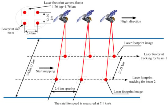
Figure 1.
Schematic of laser altimetry data from the Gaofen 7 (GF-7) satellite.
In this study, standard laser altimetry products (i.e., SLA01 and SLA03) from the GF-7 satellite obtained from the Land Satellite Remote Sensing Application Center of the Ministry of Natural Resources of China were used as experimental data. As displayed in Table 1, the main data parameters obtained by the GF-7 satellite laser system are laser footprint image data and laser echo waveform data.

Table 1.
Main data pertaining to GF-7 satellite laser system.
In previous years, several organizations have launched many Earth observation laser altimetry satellites. The technical indicators of which are listed in Table 2. Because of their design and data transmission requirements, the laser loads on the ZY-3-02 and GF-7 satellites do not acquire echo data in the atmospheric transmission range; therefore, it is impossible to detect the atmosphere using a waveform. Although the CALIOP and CATS systems have obtained data within the atmospheric transmission range, the atmospheric scattering is not corrected; this is because surface elevation is not their major detection object. However, various atmospheric parameters are used for data quality control. GLAS uses the dynamic threshold method for atmospheric detection and corrects atmospheric scattering errors according to Monte Carlo simulation results. GEDI can accurately identify data affected by atmospheric scattering and achieves data quality control using a multi-parameter constraint scheme. In the field of satellite laser altimetry, an inevitable technological breakthrough has been the migration from linear systems to photon counting systems, as well as from single beam to multi-beam systems. Compared with linear systems, photon systems do not solve the problems of atmospheric scattering identification and error correction without an echo waveform. Therefore, we attempted to identify the atmospheric scattering error by combining the characteristic parameters of the laser footprint image (LFI) and the ground echo. We then further established a novel pattern for identifying the atmospheric scattering error of the laser altimetry satellite.

Table 2.
Technical parameters of different laser altimetry satellites.
2.1. Atmospheric Scattering Error
During atmospheric transmission, the laser pulses emitted by a satellite toward the ground are affected by the scattering of particles, such as clouds and aerosols, which leads to deviations in range. For the wavelength used in spaceborne laser altimetry, the deviation caused by Mie scattering should be additionally considered. These deviations depend mainly on cloud height, COD, cloud particle size, particle shape, particle type, and the receiver field of view. Considering these factors, Duda et al. [25] analyzed the influence of single scattering on GLAS based on a Monte Carlo simulation, as shown in Figure 2. Their estimation of the delay distance is shown in Equation (1). In practice, the atmospheric scattering error is closely related to the scattering energy distribution and other factors. Laser pulses can be scattered several times at a certain height and return to the receiving field of view along various delay paths. Based on the existing theory, it is therefore difficult to accurately estimate multiple scattering.
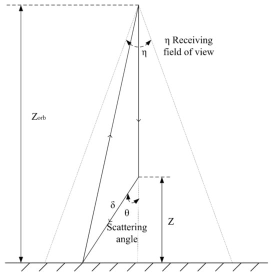
Figure 2.
Schematic diagram of atmospheric single-scattering delay [25].
As shown in Figure 2, δ is the distance from a photon to the ground through atmospheric scattering, Z is the distance from a photon to the ground without atmospheric scattering, θ is the scattering angle, η is the receiving field angle, and Zorb is the satellite orbital height. In addition, the equation is closely related to temperature, pressure, atmospheric molecular density, and other factors, which simplifies the related description to a considerable extent.
When the scattering angle is small, cos(θ) ≈ 1–θ2/2. Therefore, Equation (1) can be written as (Equation (2)):
During laser transmission, the actual scenario is far more complex than that of single scattering. Duda et al. [25] proposed an atmospheric scattering estimation model based on the scattering energy distribution function, which extends the single-scattering model to complex cases, as displayed in Equation (3):
where, represents the estimate of the average delay distance of atmospheric scattering, represents the optical depth of the atmospheric column, fg and fi represent energy components in the vertical and parallel directions, respectively, and and represent the average delay distances in the vertical and parallel directions, respectively.
Duda et al. [25] analyzed the relationship between multiple scattering errors in GLAS data and multiple parameters using Monte Carlo simulations. They summarized the data with optical depths (ODs) ranging from 0.45 to 1.1 into multiple look-up tables, which realized atmospheric scattering error calibration. However, the actual scenario is often more complicated than the model; therefore, the model can only reliably solve a few cases.
The premise of single-scattering error correction is to accurately obtain cloud and aerosol height data. Due to the superposition of backscattering effects, the total backscattering coefficient of the cloud or aerosol region is much larger than that of a sunny region. Based on this, cloud and aerosol detection can be performed by setting a reasonable threshold. This method of atmospheric detection and scattering error correction has been used by several laser altimetry satellite systems, but if the atmospheric profile data along the transmission path are not obtained, it is difficult to apply them further to the data. Based on the experimental ideas of Duda et al. [25] and the characteristics of the GF-7 satellite laser data, this study proposed new atmospheric detection and atmospheric scattering error correction methods.
2.2. Principle of Fine Cloud Detection in Laser Footprint Image
Previous studies [28,29,30] have realized cloud detection in footprint images based on SegNet and U-Net. As shown in Figure 3a, U-Net is a U-shaped network that is improved based on fully convolutional networks (FCNs). In the encoding and corresponding decoding steps, the feature images obtained by deconvolution are superimposed to obtain finer cloud contour data. However, they are accompanied by sawtooth contour noise. As shown in Figure 3b, SegNet is a symmetrical structure that, compared to FCN, improves the mapping method of the deconvolution layer and improves the spatial continuity of cloud features. However, there is a degree of false detection at the edges of the detection area. To combine the advantages of the two network structures and improve the overall accuracy, we adopted the boosting method for model ensemble generation in training [31] and test time augmentation (TTA) technology in post-processing [30]. Boosting refers to iteratively training the base model (SegNet, U-Net) and adjusting the weight ratio according to the incorrect classification results of the previous round until the training accuracies converge. The purpose of TTA technology is to enhance the typical features of the image to be detected by rotating and stretching the color mapping range without changing the model itself, thereby improving the identification accuracy.
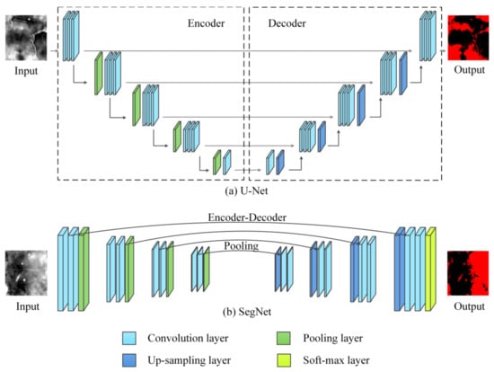
Figure 3.
Diagram of U-Net and SegNet network structures.
The boosting algorithm is a model fusion algorithm. In this study, the weights wi = 1/n, where i = 1, 2, 3,…N were initialized, where N is the number of basic models. Equation (4) was used to calculate the error rate (Errm) for each training round:
where, Gm(xi) represents the prediction and classification results of the ith basic model in the mth round. I(yi ≠ Gm(xi)) represents the probability that the ith basic model in the mth training round predicts the classification error.
Further, we calculated a sufficient matching coefficient αm, as shown in Equation (5). In this step, the weights were reasonably estimated.
Finally, the basic model weights were updated according to Equation (6), and the next round of training was started. Model fusion is expected to improve the training efficiency and has advantages for various basic network models.
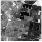
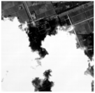
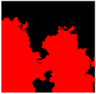
Only clouds distributed along the laser transmission path will cause errors, and the closer the cloud is located to the laser landing point, the greater the impact. Therefore, further optimization was carried out using the proposed method. The LFI records the position of the laser spot at the exit time. The position of the laser spot on the LFI can be deduced using the rational polynomial coefficient (RPC) model. Figure 4a,c exhibit the landing positions of beams 1 and 2 on the LFI, respectively, which are indicated by red dotted circles. Cloud detection was performed using 256 × 256 slices formed by expanding the predicted center position of the laser foot point by 128 pixels. The slicing range of laser beam 1 in the LFI is [line: 150–406, column: 78–334], as displayed in Figure 4b. The slicing range of laser beam 2 in the LFI is [line: 112–368, column: 147–403], as displayed in Figure 4d. However, the closer the cloud is to the center of the spot, the greater the scattering influence on the laser. Therefore, weight coefficients of 1.5, 1, and 0.5 cloud amounts were assigned to slice positions 64, 128, and 256 to quantify the influence of cloud scattering on the laser, as shown in Figure 4b,d. If the cloud amount in the slice image was greater than 30%, the slice was judged to be affected by clouds. However, if the cloud amount was less than or equal to 30%, the slice was ascertained to be unaffected by clouds.
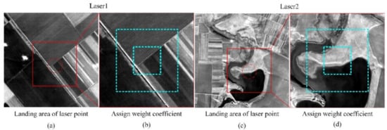
Figure 4.
Diagrams of refined cloud detection.
2.3. Fitting Multiple Regression Models Using Machine Learning
It is difficult to quantify the atmospheric scattering without data in the atmospheric transmission range for the GF-7 laser. Previous studies have indicated that atmospheric scattering causes the surface echo waveform to exhibit a tailing phenomenon and a larger pulse width variation. This is because the complex situation of atmospheric multiple scattering is related to several factors, and only a single factor is weakly correlated with these influences. In this study, we adopted the multi-layer perceptron (MLP) theory to establish a model to address this problem. MLP is a complex network model composed of numerous inter-connected nodes and includes three parts: an input layer, a hidden layer, and an output layer. All the layers are fully connected; mining of the functional relationships between multiple elements through parallel distributed information processing is often used for classification problems.
Figure 5 shows the main structure of the MLP model. N features, such as cloud coverage and waveform feature parameters, form a row matrix that is input to the input layer. The number of neurons was the same as the number of main features. Each neuron in the hidden layer weights and sums all neurons in the previous layer, corrects them using offset terms, then converts them into the next layer using the excitation function. The neurons in the output layer further weighted the sum of the output results of the hidden layer. Thus, the function result reflects the classification result of the model.
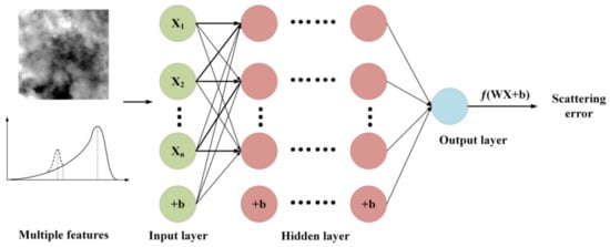
Figure 5.
Principle of the multi-layer perceptron (MLP) multiple regression model fitting process.
For a sample set with n features, the feature vector is X = [x1, x2,…xn]. There are m neurons in the hidden layer. The weight vector matrix between the input layer and the hidden layer is initialized as wmn, and the corresponding biased error is bm. The weight vector between the hidden and output layers is Wi = [w11,…wmn]. This constitutes a new input for the subsequent layer, as displayed in Equation (7).
There are m neurons in the hidden layer, the output of the ith neuron is yi, and j represents the jth characteristic, as displayed in Equation (8). f(x) represents the activation function, for which the sigmoid function was used in this study.
The neurons in the output layer perform a weighted summation on the output results of the hidden layer, the result of which is y, as displayed in Equation (9).
3. Results
3.1. Overview of GF-7 Data
The GF-7 satellite was successfully launched on 3 November 2019, and the first orbital laser data were obtained on 5 November 2019. By March 2021, 3.56 million laser points had been obtained, of which 1.57 million were in China. The global distribution of laser point trajectories is displayed in Figure 6. The observation area was concentrated in Asia, and the number of laser points in polar regions was low.
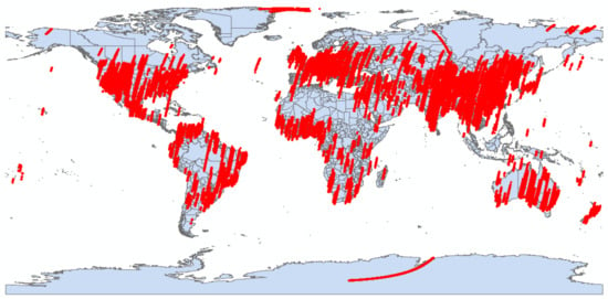
Figure 6.
Distribution of laser data obtained from the GF-7 satellite.
According to statistics of 2532 orbits and 3.56 million laser data points acquired since the GF-7 satellite was launched, the efficiency of the returning laser data was affected by the atmosphere and complex terrain. Among these, the effective laser accounted for 60.40% of the total points, the effective LFI accounted for 67.37% of the total, and the data points affected by clouds accounted for 18.47% of the total. Depending on whether a cloud is present in the laser landing area of the LFI, the laser data point affected by the cloud can be determined. Clouds have a major influence on the laser, which not only affects the data accuracy but can also invalidate the data. Table 3 shows the criteria used to determine the number of effective laser data points, the number of effective LFIs, and the number of laser data points affected by clouds.

Table 3.
Statistical index of laser data from the GF-7 satellite.
As shown in Table 4, cloud scattering influenced 18.47% of the data. As nearly 40% of the data were distributed in China, according to a quarterly classification standard of East Asia, we observed obvious seasonal changes, as displayed in Figure 7. The cloud index refers to the amount of cloud on LFI based on the method described in Section 2.2. The proportion of laser data points affected by cloud scattering during these seasons was above 30%. However, there is less cloud cover during the autumn and winter, and the proportion of laser data points affected by cloud scattering was less than 17% during these seasons. The space–time variation law of cloud cover is important for analyzing the influences of cloud scattering, planning satellite schedules, and determining the number of laser launches [19].

Table 4.
Laser data statistics since the launch of the GF-7 satellite.
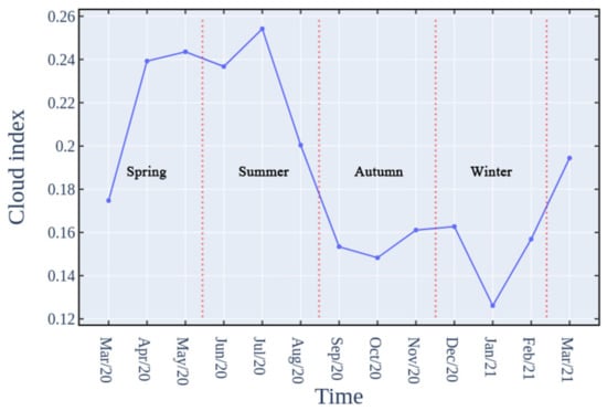
Figure 7.
Monthly statistics of laser data points affected by cloud scattering from 2020 to 2021.
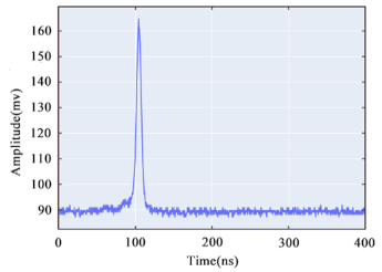
As shown in Figure 8a, satellite laser altimetry technology calculates the flight time of the laser pulse using the peak position of the transmitted waveform and the received waveform and then obtains the initial ranging value. To improve the ranging accuracy, a series of error corrections is required. The influence of atmospheric scattering is mainly reflected in two aspects: (1) as described in Section 2.1, the delay distance caused by scattering leads to a longer travel time; (2) the waveform broadening and tailing effects, as shown in the red areas of Figure 8b,d, and atmospheric scattering deform the surface echo waveform, thereby affecting the estimation accuracy of the echo peak position. As shown in Figure 8c, most satellites, including GLAS and CALIPSO, accurately identify cloud signals in noise using the dynamic threshold method; however, this cannot be implemented for the GF-7 satellite because the main detection target of GF-7 is surface elevation and the data collected during atmospheric transmission induce errors on data transmission by the satellite. Therefore, to preferentially receive the surface echo signals, a reasonable threshold value was set to remove redundant data. In summary, the GF-7 satellite data affected by scattering cannot be identified using traditional atmospheric scattering. However, atmospheric scattering has a certain influence on the ground echo waveform. Combined with actual data, neither the LFI nor the change in the echo waveform can indicate that the laser data are affected by atmospheric scattering; further, the influencing factors represented by these characteristics exhibit weak correlations with atmospheric scattering. We, therefore, designed the following experimental ideas: first, combined with the verification data, we determined whether the laser data produced height deviations; the errors caused by other factors were further eliminated, and the characteristic parameters of the footprint image and the echo waveform were extracted. Finally, an error correction model was established based on the filtered data.
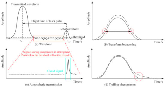
Figure 8.
Influences of atmospheric scattering on laser altimetry data. (a) shows the transmitting waveform and receiving waveform of GF-7 laser system; (b) shows the waveform broadening caused by atmospheric scattering;(c) shows the process of capturing cloud signals by laser altimetry system, but GF-7 does not have this ability; (d) shows the tailing phenomenon caused by atmospheric scattering.
3.2. Identifying Atmospheric Scattering
3.2.1. Atmospheric Scattering in Land Areas
The accuracy of land surface altimetry data is uncertain because of the presence of complex terrain in the laser spots. To effectively identify atmospheric scattering, strict screening strategies were formulated. We used airborne LiDAR point clouds provided by the inter-ministerial committee for the development of the spatial data infrastructure in North Rhine-Westphalia (NRW) as the verification data, for which the elevation accuracy reached 0.1 m. Figure 9 shows the laser footprint of the GF-7 satellite laser data in NRW, Figure 9a shows the aerial orthophoto of the study area, and Figure 9b shows the corresponding DSM data for the study area. The GF-7 satellite collected 240 laser points along five tracks in the experimental area. Based on the LFIs, we determined that 71 laser points were affected by clouds, which accounted for 29.58% of the total. The spot diameter of the GF-7 laser was 17–20 m. When the ground objects in the range of the laser spot are complex, the elevation estimation of the laser foot position will demonstrate large deviations. This causes major interference in analyses of altitude deviations caused by atmospheric scattering.
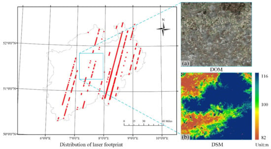
Figure 9.
Regional distributions of laser data and verification data in North Rhine-Westphalia, Germany. (a) is DOM data obtained by aerial photography in the experiment area; (b) is DSM data for LIDAR points cloud acquired in the same period.
To avoid the influence of complex terrain, as displayed in Table 5, several parameters from SLA03, a standard product of the GF-7 satellite laser altimetry data, were adopted, which strictly avoided the influence of complex topography. Although the influence of other factors can be avoided based on characteristic waveform parameters, they may still exert some influence. Therefore, it is necessary to further filter the data. As shown in Figure 10, using the reference topography data in Figure 9b, we visually determined whether the position of the laser spot was relatively flat terrain.

Table 5.
Screening indicators for land area data.
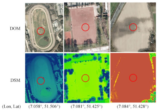
Figure 10.
Selected laser points in areas with flat terrain.
Figure 11 displays a flow chart for identifying atmospheric scattering in a land area. Using SLA 03 as input data, it was necessary to screen the wave features, LFI features, and other references to achieve accurate estimates of atmospheric scattering effects in land areas. The characteristic waveform parameters were used to eliminate the uncertainty caused by complex terrain, whereas the characteristic LFI parameters were used to determine whether atmospheric particles such as clouds and aerosols were present along the laser transmission path. Other reference features were closely related to the verification data. As mentioned in Section 3.1, atmospheric scattering affects the travel time of the laser pulse, resulting in a target height far lower than the actual value. Other references refer to key indices for determining the influence of atmospheric scattering from LiDAR data. Using the predicted laser foot point as the center, the nearest point in the point cloud with a radius (DistanceLidar) of 0.5 m was selected as the true elevation value, and the corresponding elevation error (altimeter error) of the laser point side was calculated. Due to the influence of atmospheric multiple scattering, the measured value will be lower than the target elevation, resulting in a negative deviation in the elevation measurement. After a series of steps, we determined that 62 laser points in the study area were affected by atmospheric scattering, accounting for 25.83% of the total points.
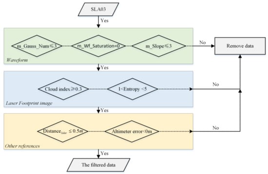
Figure 11.
Atmospheric scattering identification process for land areas.
3.2.2. Atmospheric Scattering in Water Areas
The laser data of an area are easily affected by several factors, and the influence of the terrain can be eliminated completely by screening the data using various quality control parameters. The laser elevation data for inland lakes are consistent with the surface area without being affected by wind or waves. We used laser data from Qinghai Lake, Wulungu Lake, and other inland lakes in China as experimental data to assess scattering over water. There were 115 laser spots in these areas, and their statistics are presented in Table 6. Under the influence of atmospheric scattering, determining the height deviation of a laser spot is a complicated problem, and different screening strategies were adopted for water and land areas.

Table 6.
Statistics of the experimental data from water areas.
Figure 12 shows a flow chart for atmospheric scattering identification in water areas, which differs from the screening strategy used for land areas. The characteristic parameters of LFI were used to determine whether clouds, aerosols, or other atmospheric particles were present along the laser transmission path. Characteristic meteorological parameters were used to determine whether wind waves were present on the lake surface, which could affect the consistency of the elevation data along the track. Other reference characteristics were closely related to the validation scheme. Meteorological data, including wind speed and rainfall, were obtained from hydrological stations near the lakes. For the GF-7 satellite, it is almost impossible to obtain underwater laser spots owing to the laser wavelength and emission energy [34]. When no wind or waves are present, the elevation of the inland lake area exhibits good consistency, and the average elevation of the lake surface can be used as the true value to estimate the height deviations of each laser point. When the spatial range of the lake is too large, the influence of the Earth’s curvature should be considered in the elevation changes along the track, for which there is a clear overall trend. Therefore, we fitted the water surface trend and used the fitted elevation value as the true value to calculate the corresponding altimeter errors. After a series of steps, we determined that 47 laser points were affected by atmospheric scattering in the study area, accounting for ~40.87% of the total. The height deviations ranged from 0.01 m to 1.1 m.
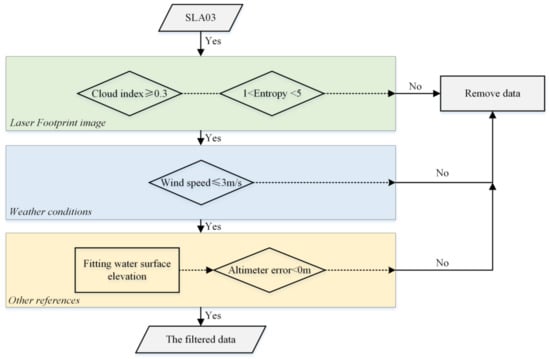
Figure 12.
Atmospheric scattering identification process for water areas.
3.2.3. Analysis of Data Characteristics Influenced by Atmospheric Scattering
After screening the atmospheric scattering data, the commonalities between the data were analyzed and the relationships among several parameters were determined. This allowed us to establish a model of atmospheric scattering identification and correction. There were 355 laser points in the study area, out of which 118 were affected by atmospheric scattering according to the above methods. GLAS is mainly used to obtain surface elevations and record atmospheric profiles with a vertical resolution lower than the surface echo waveform, which has a good ability to capture thin clouds. CALIPSO is mainly used to obtain the vertical distributions in the atmosphere. In addition, data with a higher vertical resolution supports further study of the microphysical properties of the atmosphere and can capture various types of clouds and aerosols. GF-7 differs greatly from these satellites, as it is mostly used to obtain surface elevations but cannot obtain atmospheric profiles. The GF-7 system cannot penetrate clouds with large ODs and cannot capture small cloud signals for clouds with small ODs. Therefore, the traditional atmospheric scattering identification algorithm is unsuitable for use with GF-7 laser data.
For GF-7 data, the influence of cloud scattering on the ranging accuracy is mainly divided into three aspects: (1) the laser reaches a thick cloud top, cannot penetrate the cloud, scatters back with an echo, and the received laser signal is higher than the target; (2) the laser is scattered in the clouds several times and cannot return to the receiver, so no echo or elevation angle is obtained; and (3) the laser reaches the Earth’s surface through multiple scattering by clouds, returns to the receiver along with echoes, and the received laser signal has an elevation angle lower than that of the target. Among these three cases, cases 1 and 3 are of analytical value.
As displayed in Table 7, case 1 is often accompanied by a km-scale deviation anomaly. Moreover, the scale of thick clouds often appears at the km-scale, which significantly influences the waveform signal-to-noise ratio (SNR) and the waveform width. The laser index is the unique mark of each laser point acquired by the GF-7 satellite, and further information regarding the laser point can be acquired according to this field value. The waveform SNR refers to the ratio of the effective signal-to-noise in the echo waveform, which is ~25 under normal circumstances and often decreases to ~20 under the influence of thick cloud scattering. The change in pulse width refers to the difference between the pulse width of the received waveform and that of the transmitted waveform, which reflects the change in the echo waveform width under the influence of atmospheric scattering. Under normal conditions, the change in pulse width fluctuates within 1–5 ns, and thick clouds often cause the pulse width to exceed 20 ns.

Table 7.
Laser points blocked by thick clouds.
As displayed in Table 8, case 3 occurs with an uncertain scale and in various states that are more complex than thick clouds. The laser pulse will scatter several times while penetrating thin clouds, eventually leading to ranging deviations. Distance deviations caused by multiple scattering of thin clouds are often in the order of tens of cm or can be as much as several meters. Under the influence of multiple scattering, the SNR of the echo waveforms are slightly higher than the average (25), the terrain slopes are slightly larger than the laser point data before and after the orbit, and the pulse widths change within the normal fluctuation range.

Table 8.
Influence of multiple scattering of thin clouds on the laser.
To further analyze the impact of atmospheric scattering on lakes, we selected Angzicuo Lake, an inland lake in China, as an example. Figure 13a displays the distribution of the GF-7 laser footprint at Angzicuo Lake. Figure 13b–d display the height profile, waveform SNR, and topographic slope map of Angzicuo Lake along the satellite orbit direction, respectively. In addition, their horizontal axis indicates the acquisition order of laser points along the track direction. The observation data indicate that the elevation of the track increased gradually because Angzicuo Lake is located on the Qinghai-Tibet plateau, and the terrain exhibits a trend along the track. We fitted the elevation along the track direction, removed the overall trend, and calculated the elevation deviations corresponding to each laser point using the fitted results as the actual values. The experimental results indicate that the points were particularly affected by multiple scattering, and the deviations in height measurements reached 98 cm. By combining the waveform SNR and terrain slope curve along the track, we found that the waveform SNR and slope were abnormal when the influence of atmospheric scattering was high.
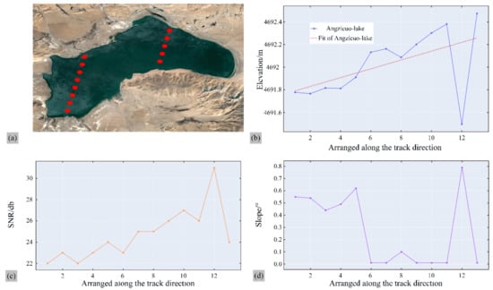
Figure 13.
Analysis of the atmospheric scattering effect in the Angzicuo Lake area. (a) is the GF-7 satellite image and laser track in the angzicuo lake; (b) is the elevation change of laser along the track direction; (c) shows the change of SNR of waveform corresponding to laser data; (d) shows the slope change corresponding to the laser data.
3.3. Atmospheric Scattering Error Correction Scheme
3.3.1. Establishing a Look-Up Table
The above analyses indicate that atmospheric scattering has a significant impact on laser altimetry data and is correlated with cloud cover, entropy, waveform SNR, terrain slope, change in pulse width, and other factors. Aiming at thin clouds that laser pulses can penetrate, atmospheric scattering error corrections are studied around data characteristics influenced by atmospheric scattering. Since GLAS has been collecting data since 2003, previous studies have determined that atmospheric scattering has a significant influence on the accuracy of laser altimetry data, and that the atmospheric scattering error has not been completely corrected by commercial data processing. Compared with the single-scattering model, multiple scattering models are more complex, and it is difficult to realize effective and accurate estimates. Currently, the most widely used commercial method uses a look-up table to correct the atmospheric scattering deviation to a certain extent. Mahesh et al. [19] found that some changes in clouds over polar regions lead to seasonal and inter-annual variations in altimetry deviations. To estimate the average height deviation for a specific period, we weighted the climatic frequencies of various cloud types based on the single-scattering Monte Carlo simulation of Duda et al. [25], the results of which are displayed in Table 9.

Table 9.
Look-up table based on polar regions of GLAS data [19]. Values are expressed in cm.
Our findings follow the seasonal variations in atmospheric scattering deviations obtained by Mahesh et al. [19]. There were obvious differences between winter (October–March) and non-winter (April–September) periods. Based on the methods of Mahesh et al. [19], we quantified the influence of cloud amount and entropy on cloud scattering, the results of which are listed in Table 10. The cloud index is the cloud amount calculated by the method described in Section 2.2, and entropy is the image entropy, as defined in Table 5. These two indexes constitute a new quality evaluation flag. When the quality evaluation flag was 1, the LFI itself may have serious quality problems, such as overexposure or imaging errors, which were not listed as data for further analysis. When the quality identification interval was 2–5, larger values presented a greater likelihood of being affected by atmospheric scattering.

Table 10.
Multiple scattering quality evaluation flags.
First, the experimental data used in Section 3.2 were classified and identified according to the indicators in Table 10. Second, the abnormal data in each flag were eliminated. Finally, the data in each flag were averaged quarterly, the statistics of which are presented in Table 11. We postulate that data with flag 1 characteristics may be greatly affected by atmospheric scattering, and may belong to data that cannot be corrected, so these data were not included in the statistics. The statistics indicate that the laser data from the GF-7 satellite are more susceptible to atmospheric scattering than those from the GLAS system, which adds greater uncertainty to altitude measurements.

Table 11.
Look-up table based on GF-7 data. Values are expressed in cm.
Applying Table 11 parameters to commercial processing methods for satellite laser altimetry data can correct the atmospheric scattering error to a certain extent and improve data availability. After correction, if the true value error is within 15 cm (water areas) or 20 cm (land areas), the measurement is regarded as corrected available laser point and the utilization rate is defined as the proportion of corrected available laser points. The statistical results are presented in Table 12. The results indicate that, according to seasonal variations in atmospheric scattering, this look-up table can improve data availability by ~20%.

Table 12.
Statistics of the results after applying scattering correction using the look-up table.
3.3.2. Atmospheric Scattering Error Correction Using the MLP Model
The look-up table can be utilized to realize an operable atmospheric scattering correction, but it cannot correct points that are significantly influenced by atmospheric scattering. In addition, because of the complexity and diversity of atmospheric scattering, uneven ranging errors are distributed from small to large in each flag. The look-up table can only solve common data problems for each flag, but it cannot provide the best solution for every scenario. Some laser points that are not affected by atmospheric scattering will also be corrected erroneously, which may cause potential ranging deviations. After analyzing several cases, the results indicate a weak correlation between altitude deviations caused by atmospheric scattering and cloud cover, waveform SNRs, and other factors. The best correlation occurs when the waveform SNR reaches 40%, followed by when cloud cover is 36%. Therefore, it is difficult to theoretically deduce the relationship between these elements. To address this, we used the MLP algorithm.
Characteristic parameters, including cloud cover, information entropy, waveform SNR, terrain slope, and changes in wave width, of each laser point were used as inputs, and the height deviations were determined. Because the overall goal is to determine the influence of atmospheric scattering under thin cloud conditions, all points with positive height deviation were zero, and all points with negative height deviations were used directly. Because we obtained a small amount of data, it was difficult to obtain better results using MLP; therefore, we adopted several strategies to enhance the data. Parameters such as waveform SNR, terrain slope, and changes in wave width under the influence of atmospheric scattering often change dynamically within a certain range. Based on this, each parameter input value was increased or decreased by a reasonable random number and the number of samples was increased from 355 to 3000.
Table 13 shows the statistics of the results after the application of atmospheric scattering correction using the MLP model. Compared with the look-up table, the MLP model yielded a higher identification accuracy for laser points that were not affected by atmospheric scattering, and the overall data availability after correction was improved by 5%. In addition, using the screening strategy described in Section 3.2.2, we selected laser data from the Xingkai Lake area along the border between China and Russia and created a test dataset. The results indicate that the model worked well in other areas, and the availability of data affected by atmospheric scattering improved to 25%, which indicates that the model has good generalization ability. However, this model can be further improved by fitting the model to other characteristic parameters that are more closely related to atmospheric scattering and have larger influences, or by constructing a sample dataset with richer characteristics.

Table 13.
Statistics of scattering correction results for the Xingkai Lake area using the MLP model.
4. Conclusions
Centimeter-scale elevation data can be obtained using satellite laser altimetry, and the forward scattering effect caused by single/multiple atmospheric scattering leads to deviations in altimetry that cannot be ignored. The GF-7 satellite is the first Chinese satellite to carry an official laser altimeter payload, and the first satellite to realize stereo mapping by combining laser altimetry and optical images globally. Based on the GF-7 laser data, the influence of atmospheric scattering on its ranging accuracy was analyzed. The main conclusions of this study are:
- We systematically combed the atmospheric scattering identification and correction schemes adopted by existing laser altimetry systems and analyzed feasible atmospheric scattering identification and correction methods according to the characteristics of the GF-7 data.
- We found that the GF-7 laser data were affected by atmospheric scattering and complex terrain. Nearly 40% of the data did not receive echoes, whereas 18.47% of the received data were affected by atmospheric scattering, which can lead to meter-scale maximum height deviations that considerably affect the laser data availability.
- The influence of atmospheric scattering on the laser data was analyzed. The results indicate that a weak correlation exists between atmospheric scattering and cloud cover, entropy, waveform SNR, terrain slope, and changes in pulse width.
- Using the statistics of long-term time series data, we found that the atmospheric scattering effect of the GF-7 data had obvious seasonal variations. The errors from April to September were large (~20 cm), whereas the errors were small from October to March (~10 cm).
- Based on the above conclusions, and according to the characteristics of the GF-7 data, we proposed two scattering correction methods: a look-up table and MLP model construction. The results indicate that the look-up table can correct the atmospheric scattering error, and the data availability after correction reached 16.67% and 26.09% for land and water areas, respectively. A disadvantage of the look-up table is that a few laser points not scattered by the atmosphere were corrected in error. The atmospheric scattering identification and correction model established using MLP improved the data availability to 21% and 30% for land and water areas, respectively, which is ~5% higher than those of the look-up table. Thus, the identification accuracies, which were low due to atmospheric scattering, were improved.
Author Contributions
J.Y. and G.L. proposed the methodology and wrote the manuscript. X.T. and Z.Z. contributed to improving the methodology and is the corresponding author. J.C. and B.A. helped edit and improve the manuscript. S.Z. and J.G. contributed to methodological testing. All authors have read and agreed to the published version of the manuscript.
Funding
This research was jointly supported by grants from the Application Demonstration System of GaoFen Remote Sensing Mapping of China (No. 42-Y30B04-9001-19/21) and the Project of the National Natural Science Foundation of China (Nos. 41971425 and 41871382).
Data Availability Statement
The data are not publicly available due to restrictions privacy.
Acknowledgments
The authors would like to thank the Land Satellite Remote Sensing Application Center for providing the GF-7 satellite data and the inter-ministerial committee for the development of the spatial data infrastructure in North Rhine-Westphalia for providing high-resolution and LiDAR data of North Rhine-Westphalia area.
Conflicts of Interest
The authors declare no conflict of interest.
References
- Li, G.; Tang, X.; Zhang, C.; Zhang, C. Multi-criteria constraint algorithm for selecting ICESat/GLAS data as elevation control points. J. Remote Sens. 2017, 21, 96–104. [Google Scholar]
- Tang, X.; Li, G. Development and prospect of laser altimetry satellite. Space Int. 2017, 11, 13–18. (In Chinese) [Google Scholar] [CrossRef]
- Zwally, H.; Schutz, B.; Abdalati, W.; Abshire, J.; Bentley, C.; Brenner, A.; Bufton, J.; Dezio, J.; Hancock, D.; Harding, D.; et al. ICESat’s laser measurements of polar ice, atmosphere, ocean, and land. J. Geodyn. 2002, 34, 405–445. [Google Scholar] [CrossRef] [Green Version]
- Wang, X.; Cheng, X.; Gong, P.; Huang, H.; Li, Z.; Li, X. Earth science applications of ICESat/GLAS: A review. Int. J. Remote Sens. 2011, 32, 8837–8864. [Google Scholar] [CrossRef]
- Li, G.; Guo, J.; Pei, L.; Zhang, S.; Tang, X.; Yao, J. Extraction and Analysis of the Three-Dimensional Features of Crevasses in the Amery Ice Shelf Based on ICESat-2 ATL06 Data. IEEE J. Sel. Top. Appl. Earth Obs. Remote Sens. 2021, 14, 5796–5806. [Google Scholar] [CrossRef]
- Yang, F.; Wen, J.; Wang, W.L. Application progress and prospect of ICESat and ICESat-2. Chin. J. Polar Res. 2011, 23, 138–148. [Google Scholar]
- Yu, A.W.; Stephen, M.A.; Li, S.X.; Shaw, G.B.; Seas, A.; Dowdye, E.; Troupaki, E.; Liiva, P.; Poulios, D.; Mascetti, K. Space laser transmitter development for ICESat-2 mission. In Proceedings of the Solid State Lasers XIX: Technology and Devices, San Francisco, CA, USA, 24–28 January 2010; Volume 7578, p. 757809. [Google Scholar]
- Xie, D.; Li, G.; Zhao, Y.; Yang, X.; Tang, X.; Fu, A. GEDI space-based laser altimetry system and its application in the United States. Space Int. 2018, 12, 39–42. (In Chinese) [Google Scholar]
- Li, G.; Tang, X. Analysis and Validation of ZY-3 02 Satellite Laser Altimetry Data. Acta Geodet. Cart. Sin. 2017, 46, 1939–1949. [Google Scholar]
- Li, G.; Gao, X.; Chen, J.; Zhao, Y.; Mo, F.; Zhang, Y. Data quality analysis of ZY-3 02 satellite laser altimeter. J. Remote Sens. 2019, 23, 1159–1166. (In Chinese) [Google Scholar] [CrossRef]
- Tang, X.; Xie, J.; Liu, R.; Huang, G.; Zhao, C.; Zhen, Y.; Tang, H.; Dou, X. Overview of the GFLaser Altimeter System Mission. Earth Space Sci. 2019, 7. (In Chinese) [Google Scholar]
- Li, G.; Guo, J.; Tang, X.; Ye, F.; Zuo, Z.; Liu, Z.; Chen, J.; Xue, Y. Preliminary Quality Analysis of Gf-7 Satellite Laser Altimeter Full Waveform Data. Int. Arch. Photogramm. Remote Sens. Spat. Inf. Sci. 2020, 43, 129–134. [Google Scholar] [CrossRef]
- Smith, D.E.; Zuber, M.T.; Neumann, G.; Lemoine, F.G.; Mazarico, E.; Torrence, M.H.; McGarry, J.F.; Rowlands, D.D.; Head, J.W.; Duxbury, T.H.; et al. Initial observations from the Lunar Orbiter Laser Altimeter (LOLA). Geophys. Res. Lett. 2010, 37, 1–6. [Google Scholar] [CrossRef]
- Head, J.W.; Kreslavsky, M.; Hiesinger, H.; Ivanov, M.; Pratt, S.; Seibert, N.; Smith, D.E.; Zuber, M.T. Oceans in the past history of Mars: Tests for their presence using Mars Orbiter Laser Altimeter (MOLA) data. Geophys. Res. Lett. 2013, 25, 4401–4404. [Google Scholar] [CrossRef] [Green Version]
- Li, G. Earth Observing Satellite Laser Altimeter Data Processing Method and Engineer Practice; Wuhan University: Wuhan, China, 2017. [Google Scholar]
- Zhang, Y.; Sun, X. Analysis on the Influence Factors of Laser Active Detection Technology. Semicond. Optoelectron. 2016, 37, 882–885. [Google Scholar]
- Yang, R.; Ma, C.; Han, X.; Su, Z.; Jian, D. Study of the attenuation characteristics of laser propagation in the atmosphere. Infrared Laser Eng. 2007, 36, 415–418. [Google Scholar]
- Platt, C.M.R. Remote Sounding of High Clouds. III: Monte Carlo Calculations of Multiple-Scattered Lidar Returns. J. Atmos. Sci. 1981, 38, 156–167. [Google Scholar] [CrossRef] [Green Version]
- Mahesh, A.; Spinhirne, J.; Duda, D.; Eloranta, E. Atmospheric multiple scattering effects on GLAS altimetry. II. Analysis of expected errors in Antarctic altitude measurements. IEEE Trans. Geosci. Remote Sens. 2002, 40, 2353–2362. [Google Scholar] [CrossRef]
- Lancaster, R.S.; Spinhirne, J.D.; Palm, S.P. Laser pulse reflectance of the ocean surface from the GLAS satellite lidar. Geophys. Res. Lett. 2005, 32, 109–127. [Google Scholar] [CrossRef]
- Brenner, A.C.; DiMarzio, J.P.; Zwally, H.J. Precision and Accuracy of Satellite Radar and Laser Altimeter Data Over the Continental Ice Sheets. IEEE Trans. Geosci. Remote Sens. 2007, 45, 321–331. [Google Scholar] [CrossRef]
- Chen, S.; Li, Z.; Chen, M.; Hu, L.; Zhou, H. Influence of atmospheric multiple scattering effects on the range bias for satellite laser altimeter. Infrared Laser Eng. 2012, 41, 2522–2526. [Google Scholar]
- Yao, J.; Gao, X.; Li, G.; Yang, X.; Lu, J.; Li, C. Cloud optical depth inversion based on ICESat/GLAS echo energy data. Infrared Laser Eng. 2019, 48, 132–140. [Google Scholar]
- Tang, X.; Yao, J.; Li, G. Influence of cloud scattering on satellite laser altimetry data and its correction. Appl. Optics 2020, 59, 4064–4075. [Google Scholar] [CrossRef] [PubMed]
- Duda, D.; Spinhirne, J.; Eloranta, E. Atmospheric multiple scattering effects on GLAS altimetry. I. Calculations of single pulse bias. IEEE Trans. Geosci. Remote Sens. 2001, 39, 92–101. [Google Scholar] [CrossRef]
- Yang, Y.; Marshak, A.; Palm, S.P.; Wang, Z.; Schaaf, C. Assessment of Cloud Screening With Apparent Surface Reflectance in Support of the ICESat-2 Mission. IEEE Trans. Geosci. Remote Sens. 2013, 51, 1037–1045. [Google Scholar] [CrossRef]
- Michelle, H.; Story, S.; Yi, D. Algorithm Theoretical Basis Document for GEDI Transmit and Receive Waveform Processing for L1 and L2 Products, Goddard Space Flight Center. 2019. Available online: https://gedi.umd.edu (accessed on 12 December 2021).
- Yao, J.; Tang, X.; Li, G.; Guo, J.; Chen, J.; Yang, X.; Ai, B. Cloud detection of GF-7 satellite laser footprint image. IET Image Process. 2021, 5, 1–8. [Google Scholar] [CrossRef]
- Badrinarayanan, V.; Kendall, A.; Cipolla, R. SegNet: A Deep Convolutional Encoder-Decoder Architecture for Image Segmentation. IEEE Trans. Pattern Anal. Mach. Intell. 2017, 39, 2481–2495. [Google Scholar] [CrossRef]
- Ronneberger, O.; Fischer, P.; Brox, T. U-Net: Convolutional networks for biomedical image segmentation. In International Conference on Medical Image Computing and Computer-Assisted Intervention; Springer: Cham, Switzerland, 2015; pp. 234–241. [Google Scholar] [CrossRef] [Green Version]
- Buhlmann, P.; Yu, B. Additive Logistic Regression: A Statistical View of Boosting: Discussion. Ann. Statistics 2000, 28, 377–386. [Google Scholar]
- Zuo, Z.; Tang, X.; Li, G.; Ma, Y.; Zhang, W.; Li, S. Inversion of Terrain Slope and Roughness with Satellite Laser Altimeter Full-Waveform Data Assisted by Shuttle Radar Topographic Mission. Remote Sens. 2021, 13, 424. [Google Scholar] [CrossRef]
- Abutaleb, A.S. Automatic thresholding of gray-level pictures using two-dimensional entropy. Comput. Vision Graph. Image Process. 1989, 47, 22–32. [Google Scholar] [CrossRef]
- Huang, T. Analysis of ICESat/GLAS Waveform and Identification of Its Observation upon Water. J. Yangtze River Sci. Res. Inst. 2018, 35, 159–162. (In Chinese) [Google Scholar]
Publisher’s Note: MDPI stays neutral with regard to jurisdictional claims in published maps and institutional affiliations. |
© 2021 by the authors. Licensee MDPI, Basel, Switzerland. This article is an open access article distributed under the terms and conditions of the Creative Commons Attribution (CC BY) license (https://creativecommons.org/licenses/by/4.0/).
