Satellite–Derived Topography and Morphometry for VHR Coastal Habitat Mapping: The Pleiades–1 Tri–Stereo Enhancement

Abstract

The evolution of the coastal fringe is closely linked to the impact of climate change, specifically increases in sea level and storm intensity. The anthropic pressure that is inflicted on these fragile environments strengthens the risk. Therefore, numerous research projects look into the possibility of monitoring and understanding the coastal environment in order to better identify its dynamics and adaptation to the major changes that are currently taking place in the landscape. This new study aims to improve the habitat mapping/classification at Very High Resolution (VHR) using Pleiades–1–derived topography, its morphometric by–products, and Pleiades–1–derived imageries. A tri–stereo dataset was acquired and processed by image pairing to obtain nine digital surface models (DSM) that were 0.50 m pixel size using the free software RSP (RPC Stereo Processor) and that were calibrated and validated with the 2018–LiDAR dataset that was available for the study area: the Emerald Coast in Brittany (France). Four morphometric predictors that were derived from the best of the nine generated DSMs were calculated via a freely available software (SAGA GIS): slope, aspect, topographic position index (TPI), and TPI–based landform classification (TPILC). A maximum likelihood classification of the area was calculated using nine classes: the salt marsh, dune, rock, urban, field, forest, beach, road, and seawater classes. With an RMSE of 4 m, the DSM#2–3_1 (from images #2 and #3 with one ground control point) outperformed the other DSMs. The classification results that were computed from the DSM#2–3_1 demonstrate the importance of the contribution of the morphometric predictors that were added to the reference Red–Green–Blue (RGB, 76.37% in overall accuracy, OA). The best combination of TPILC that was added to the RGB + DSM provided a gain of 13% in the OA, reaching 89.37%. These findings will help scientists and managers who are tasked with coastal risks at VHR.

1. Introduction

1.1. Global Change

Coastal landscapes have faced significant changes over billions of years, and their evolution is concomitant with major climatic upheavals. In its sixth and most recent report, the Intergovernmental Panel on Climate Change (IPCC) indicates that climate change is occurring more rapidly than originally predicted, with unprecedented increases in sea levels, heat waves, and the faster melting of polar ice caps [1]. Currently, mankind is trying to cope with and adapt to rapid climate changes that influence ocean currents, winds, precipitations, temperatures, and strongly re–shaped landscapes [2].

1.2. Landuse/Landcover Observation Techniques

Observation techniques for tracking landscape changes are many and varied. At local–scale and very–high (VH) spatial resolution, unmanned aerial vehicles (UAV) are useful for the VH temporal resolution monitoring of coastal socio–ecosystems [3]. UAVs are cost–efficient and easily deployable for shoreline detection [4] and for the identification of seasonal variations in saltmarsh meadows [5]. They are, however, not well suited for monitoring areas at the landscape scale (several km²) due to not only the restrictions that are imposed by legislation but also the technical limitations that are enforced by the number of flight times that are permitted by the battery capacity. In addition, in coastal areas, the meteorological and marine conditions require a maximum time of presence on the site due to the tides (±one hour after low water slack).

Manned aerial vehicles (MAV) serve as a robust alternative that leverages passive sensors with a basic red–green–blue (RGB) spectrum and sometimes the infrared spectrum [6] or an active light detection and ranging (LiDAR) sensor [7]. The complete solution makes it difficult to plan missions, and sensors such as LiDAR are rather expensive.

1.3. Spaceborne Acquisition and Stereoscopy

Yet, the analysis of the environment at the landscape scale is made possible by satellites which have a VH spatial, a multispectral, and even a hyperspectral resolution for the best–equipped satellites [8].

A spaceborne solution exists to obtain multispectral VH resolution images that are 0.50 m and 0.30 m pixels in size, which are provided by Pleiades–1 or WorldView–3 and 4, respectively. Satellite–based multispectral VH resolution mapping of the coastal fringe has been successfully performed in studies focusing on tropical [9] or temperate environments [10].

Since 2000, some remote sensing satellites that are specialized in stereo acquisition have been launched into orbit around the Earth, such as the Worldview–1, –2, –3, –4 constellations, GeoEye–1 and –2, the Pleiades–1 and, –1B constellations, and the 2021–launched Pleiades Neo, whose images are not yet available for research at the time of this submission [11]. The operating principle of stereoscopy is to photograph an object or a landscape from two different angles in the same way as human vision is able to, with a specific overlap for determining the 3D information of the obtained images. Sometimes a third angle (nadir) of view can be available as a redundant observation to increase the accuracy when producing a digital elevation or surface model.

Satellite–based stereo topography has the capability of improving coastal mapping by improving the spectral discrimination of eco–geo–morphological objects [12]. However, when a tri–stereo product is used, do they augment/boost this coastal mapping? Do the morphometric parameters that are derived from the topography contribute to a better classification of coastal ecosystems than basic spectral information? This paper along with the experimental results that are presented in it will seek to answer these two questions.

2. Materials and Methods

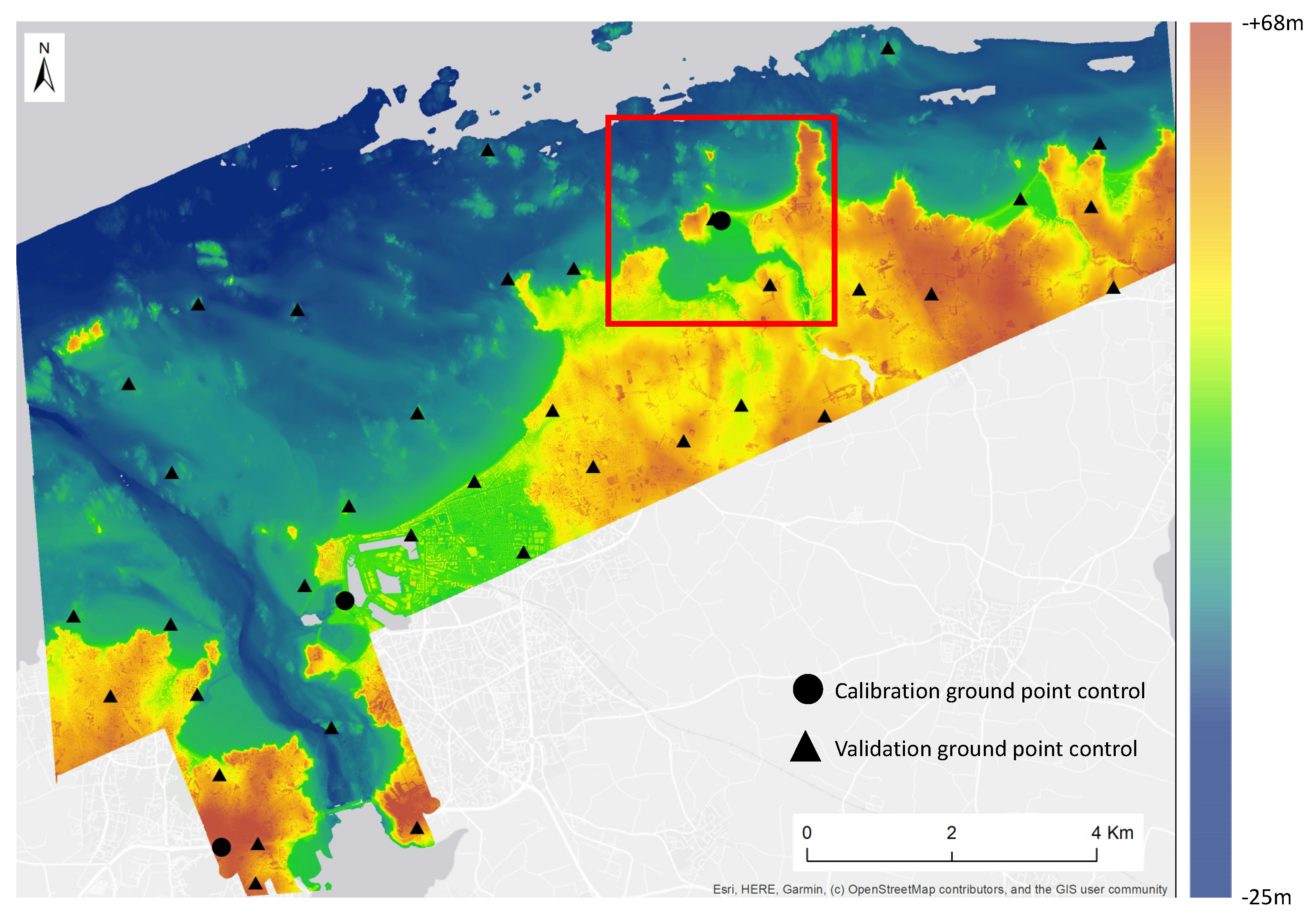
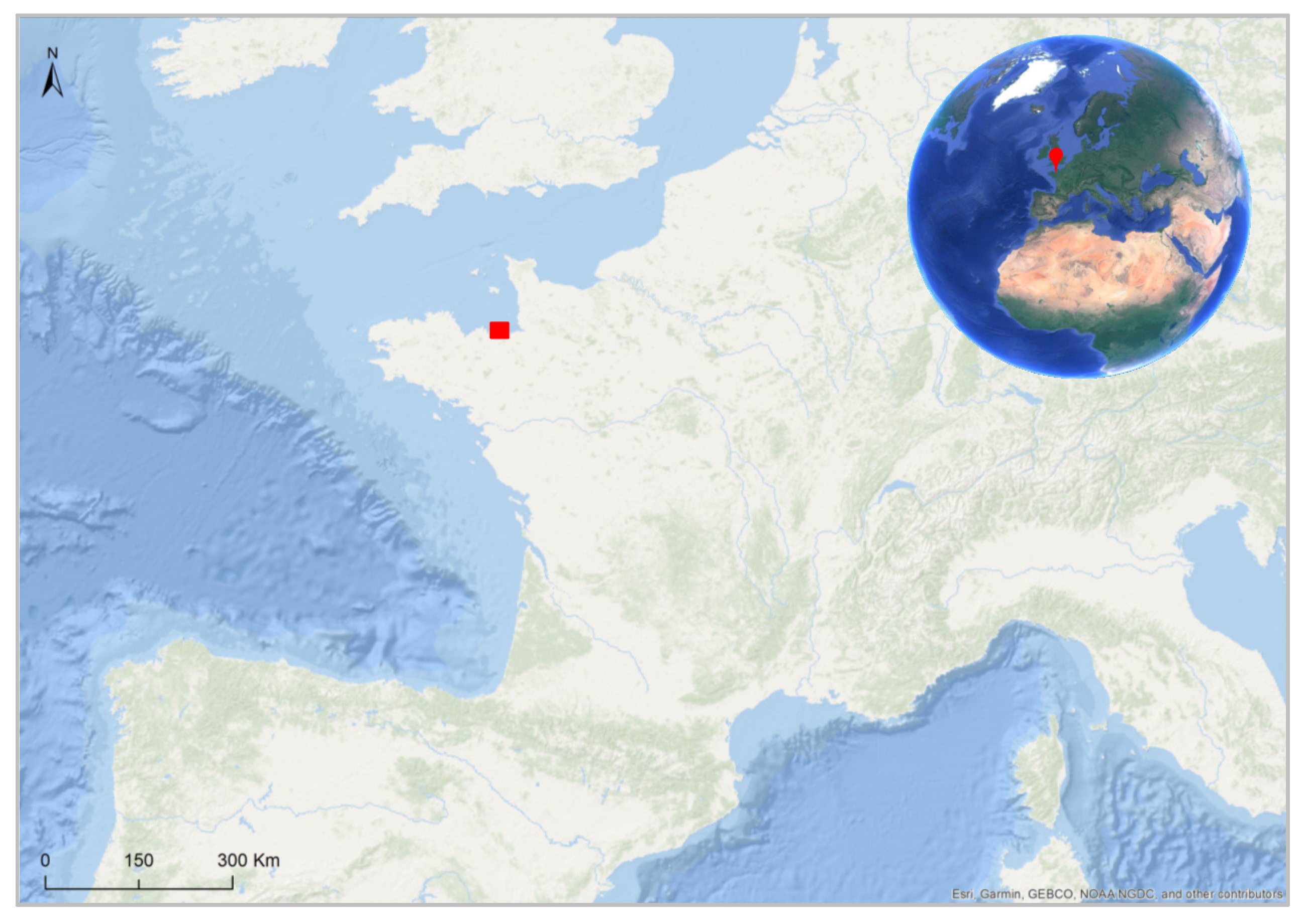
2.1. The Study Site

The entire study site (76 km² terrestrial part) is located on the Emerald Coast in Brittany (France) along the Channel Sea (48.60° N, 2.00° W; Figure 1). It is characterized by a diversity of ecosystems that are shaped by the proximity of a megatidal sea and is one of the six areas with the highest tidal ranges in the world (up to 14 m) [13]. The Rance, a coastal river, ends its course in the bay of Saint Malo, dividing the area in two sub–sites. In terms of land cover, this study area is composed of temperate zone coastal vegetation, salt marshes, rocks, dunes, and fine sand beaches. The coastline is strongly indented, leaving multiple sandy beaches surrounded by rocky points and islets a little further offshore. Bays are also common on this coastal fringe and are featured by the presence of salt marsh meadows. In terms of urbanism, this Brittany coastal fringe is subject to strong anthropic pressures. The small fishing villages of the past have evolved into resort urban areas that now attract tourists in search of iodized air and marine landscapes.

Figure 1. Location of the study on the Emerald Coast (France).

As with all coastal areas in the world, the Emerald Coast is not exempted from coastal risks. Its highly populated coastline increases the vulnerability of lowland populations.

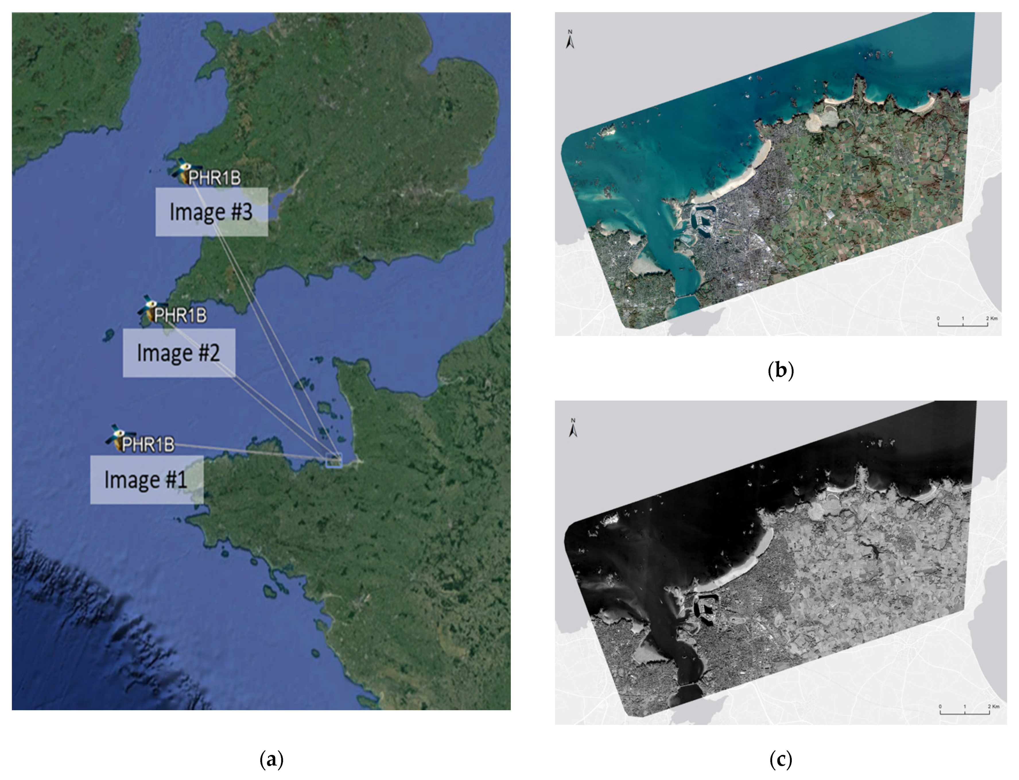
2.2. Pleiades–1 Satellite Imageries

The Pleiades–1A and 1B constellation multispectral satellites were launched on 16 December 2011 and 2 December 2012, respectively [14]. The Pleiades–1 constellation acquires images of the Earth daily and can cover up to 1,000,000 km² per day. The radiometric spectrum of the sensor extends from 430 nm to 940 nm (B: 430–550 nm; G: 500–620 nm; R: 590–710 nm; and NIR: 740–940 nm).

Data collection is based on tri–stereo images from the Pleiades–1 satellite sensor (Table 1; Figure 2a). The satellite orbited over the study area on 28 November 2020 to collect three images at 11 h 26 min 14 s (UTC), then at 11 h 26 min 24 s (UTC), and finally at 11 h 26 min 32 s (UTC; Table 1). Each dataset of images contains panchromatic and multi–spectral images (R, G, B, NIR) that are 0.5 m and 2 m pixels in size, respectively (Table 1, Figure 2b,c). The images were delivered without initial geometric processing (primary level) and without radiometric processing.

Table 1. Pleiades–1 specificities of the tri–stereo acquisitions over the study site.

Parameters	Image #1	Image #2	Image #3
Acquisition date	28 November 2020	28 November 2020	28 November 2020
Time	11 h 26 min 14 s	11 h 26 min 24 s	11 h 26 min 32 s
Image orientation angle (in degree)	180.01	180.03	180.01
Incidence angle (in degrees)	16.41	15.35	16.05
Sun azimuth (in degree)	172.60	172.60	172.60
Sun elevation (in degree)	19.77	19.77	19.77

Figure 2. Viewing directions with respect to the target area of the tri–stereo Pleiades–1 images (a); natural–coloured nadiral imagery at 2 m pixel size (b), and panchromatic nadiral imagery at 0.5 m pixel size (c) of the study site.

2.3. LiDAR Airborne Dataset

Thanks to multiple LiDAR data acquisition campaigns on the French territory by the French Navy’s Hydrographic and Oceanographic Department (SHOM), a LiDAR point cloud was available for the study site. The land/sea continuum is guaranteed by the precision of the topo–bathymetric dataset (horizontal and vertical topographic accuracy of 0.20 m), which was acquired with a Leica HawkEye–3 sensor (Chiroptera + Deep channel).

The 2018 LiDAR point cloud was used to calibrate and validate the digital elevation model (DEM) using 36 validation points that were evenly distributed over the study area. The coordinates in XY (WGS84 UTM 30N) and Z (ellipsoidal height) were extracted for each point (Figure 3).

Figure 3. 2018 LiDAR of Emerald Coast with evenly distributed calibration points (black circle) and validation points (black triangle); the red rectangle corresponds to the sub–study site.

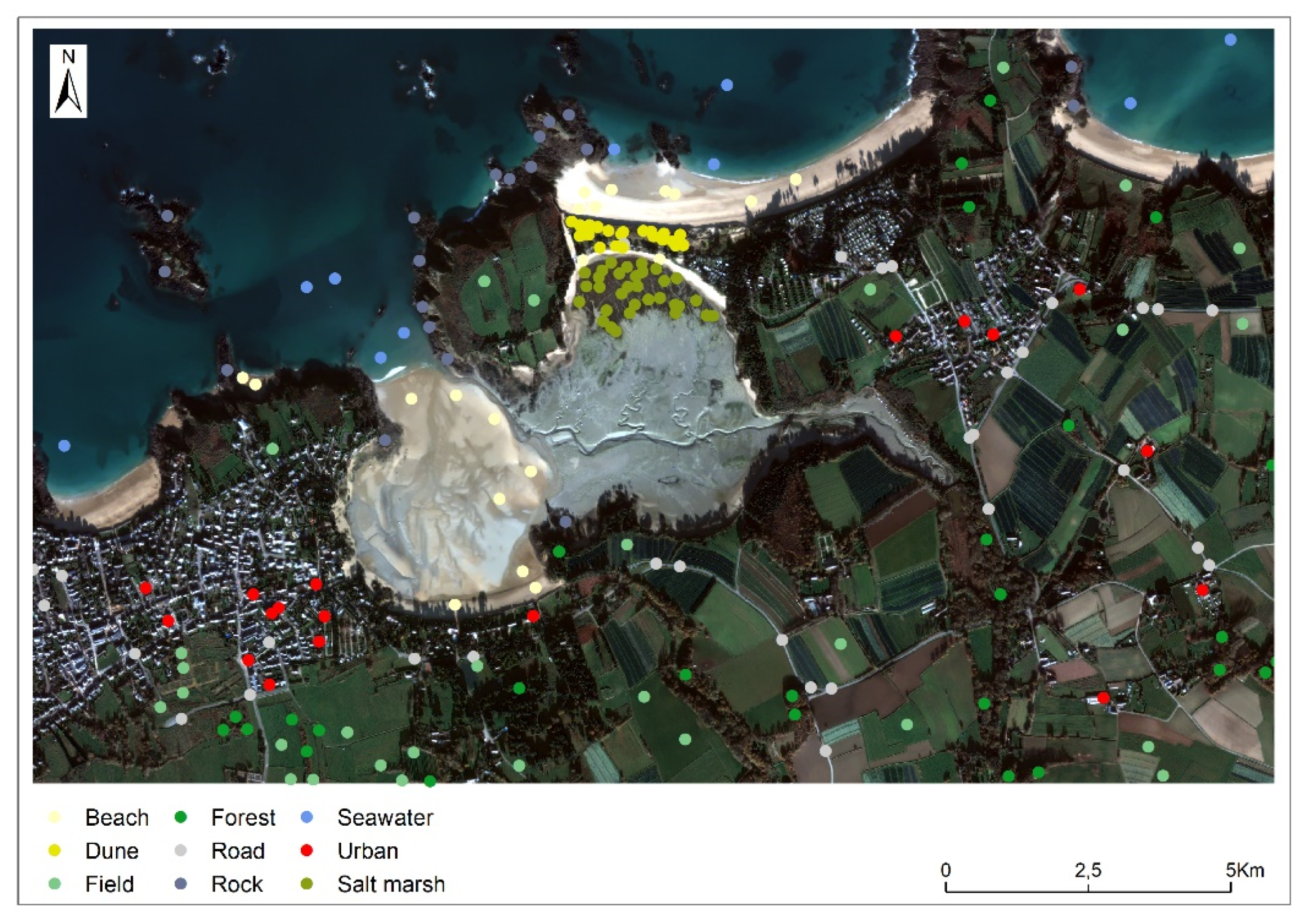
2.4. Coastal Landscape Classes

Nine classes that are representative of the coastal landscape were identified (Table 2, Figure 4): dune (white dune vegetation Ammophila arenaria), salt marsh (salt marsh vegetation composed mainly of Spartina, Salicornia, Suaeda, and Halimione portulacoides), rock, urban (building roof), forest (mix of deciduous and coniferous), field (cultivated and uncultivated), beach (wet and dry sand of grain of 0.06 to 2 mm), road (mainly asphalt), and seawater (shallow to deep salt water). A sub–study site was extracted for the classification tests (red rectangle in Figure 3).

Table 2. Pleiades–1 natural–coloured thumbnail of the nine coastal landscape classes.

Class Name	Thumbnail
Dune
Salt marsh
Rock
Urban
Forest
Field
Beach
Road
Seawater

Figure 4. Natural–coloured nadiral Pleaide–1 imagery with the calibration/validation class locations.

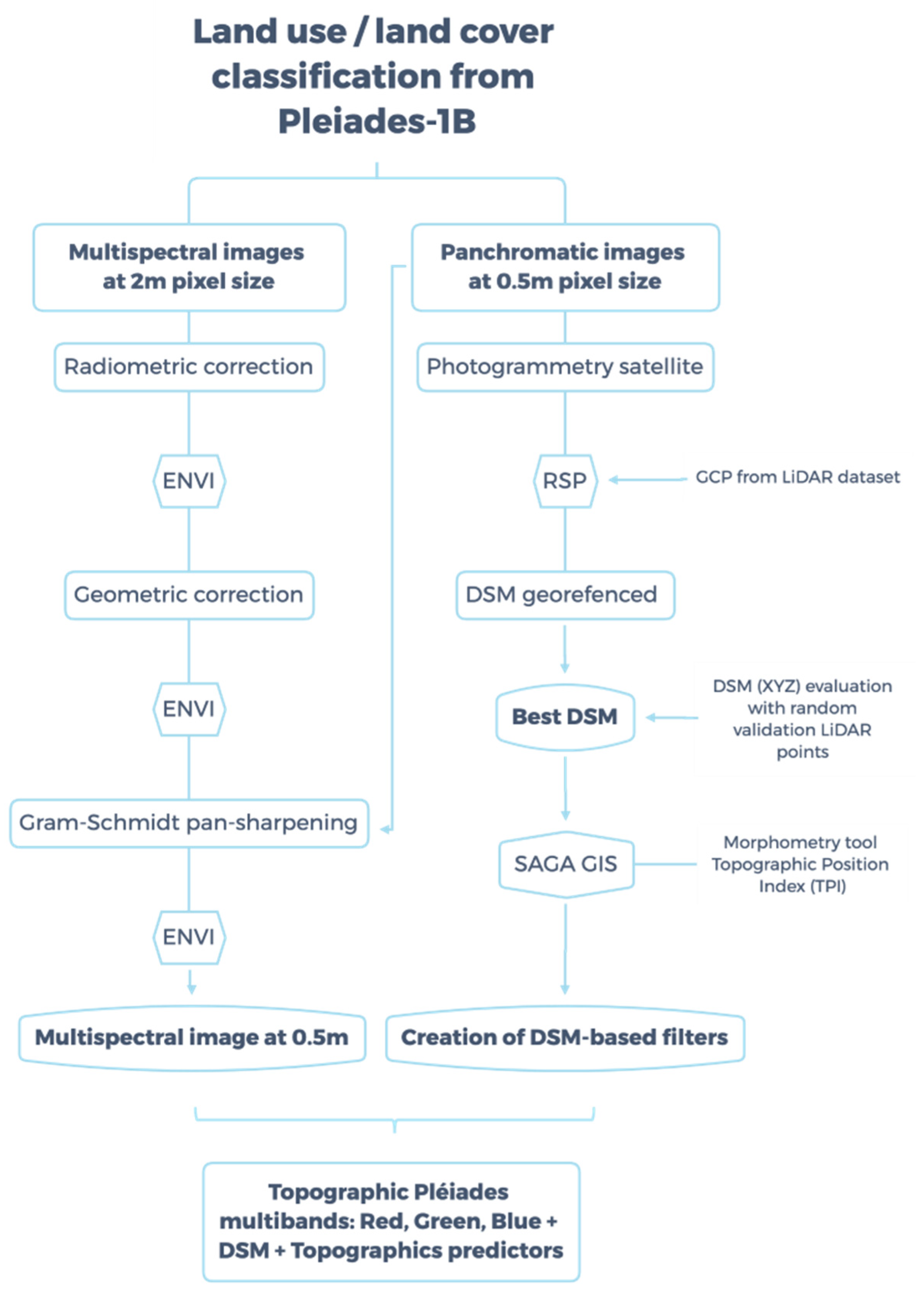
2.5. Satellite–Derived Topography: Photogrammetry Reconstruction

Three couples of panchromatic images, which were characterized by three intersection angles, were processed using the opensource software RSP (RPC stereo processor, [15], Figure 5) from the tri–stereo images from Pleiades–1. RSP was used to process stereo satellite images so as to create point dense clouds and then to create a Digital Surface Model (DSM) using the photogrammetry technique. For each pair of images, RSP used the Rational Polynomial Coefficients (RPC) files, which were delivered with the Pleiades–1 images, which contain the geometric parameters for the same images to build the projection relationship between the 3D and 2D space. The additional Ground Control Points (GCP) increased the accuracy of the reconstruction horizontally and vertically.

Figure 5. Flowchart describing methodology for coastal landscape classification from Pleiades–derived topography and morphometry.

Three image pairs (1) without, (2) with 1, or (3) with 3 GCP (DSM#2–3_0, DSM#2–3_1, DSM#2–3_3, DSM#1–2_0, DSM#1–2_1, DSM#1–2_3, DSM#1–3_0, DSM#1–3_1, DSM#1–3_3) were computed using RSP, and nine DSM were evaluated using the root mean square error (RMSE). The lowest RMSE was the factor that identified what the best photogrammetry–based DSM was.

$$RMSE=\sqrt{\frac{{{\displaystyle \sum }}_{i=1}^n{\left(Pi-Oi\right)}^2}{n}},$$

(1)

where P is the value of the calculated DSM ellipsoidal height; O is the value of the LiDAR ellipsoidal height; and n is the number of observations.

In addition, the DSMs were also evaluated at the ecosystem scale by referring to the nine identified classes. A mean of the ellipsoidal heights per class was calculated, and a dispersion parameter such as standard deviation was determined to show the homogeneity or heterogeneity of the statistical series.

The MS images underwent three pre–processing stages before they were integrated into the analyses:

ENVI’s FLAASH tool was used to correct the influence of the atmosphere (top of atmosphere, TOA) for each pixel in the images. The radiometric correction of the MS images consisted of converting the numerical radiance values into TOA reflectance values. The reflectance was calculated according to the radiance/irradiance (solar) ratio.

The MS images were also geometrically corrected using both the RPC files and the DSMs, which had been created previously from the panchromatic stereo images. This pre–processing stage corrected the distortions in the images that were related to the positioning of the satellite or the structure of the landform.

The MS images were pan–sharpened using the Gram–Schmidt algorithm. It resampled the 2 m pixel size of the MS image to be of the 0.5 m pixel size of the panchromatic images (see James et al., 2021).

2.6. Satellite–Derived Morphometry

The morphometric features such as slope, aspect, topographic position index (TPI), and TPI–based landform classification (TPILC) were calculated from the best DSMs using the SAGA GIS opensource software (Figure 5) [16]. These indicators that were related to the topography of the study site were coupled with the basic RGB spectral information to reveal the contributions of each predictor. The near–infrared band of the image was also compared to the morphometric predictors.

The slope highlights the inclination of a pixel, and this aspect defines the orientation of the slope from a compass direction. The slope and aspect predictors generate raster images that are computed from the DSM. The percentage of slope is the ratio between the difference in altitude and the horizontal distance. A 3 × 3 pixel moving window compares the values of a pixel around its neighbors to define the slope percentage.

TPI computes the elevation or altitude of each pixel and subtracts it from the mean elevation or altitude of a neighborhood of that pixel of a grid raster [17]. Values that are lower than 0 correspond to valleys. Values higher than 0 are ridges, and those that are around 0 are flat areas. TPI–based landform classification was founded on the same principle as the basic TPI. Two different scales were combined to allow for the better identification of the topographic differences [18].

2.7. Classification Algorithm

A supervised machine learning classifier algorithm was tested: maximum likelihood (ML) with ENVI^® software (Figure 5) [19]. ML is a probabilistic method that calculates the variance and covariance of each class by assuming that the statistics of each class in each band are normally distributed. A pixel is then assigned to the class with the most likely probability of membership.

An array of 500 calibration pixels and 500 validation pixels per class were extracted from the satellite–derived products (Table 2). Overall accuracy (OA) is determined as the sum of the correctly classified pixels divided by the number of pixels. The producer accuracy (PA) corresponds to the accuracy of the map from the producer’s point of view, i.e., from the algorithm. The result expressed in % indicates the fraction of correctly classified pixels of those that are known to belong to the class [20]. The OA of each by–product combination was evaluated through the calibration/validation pixels that were calculated with the confusion matrix.

3. Results

After the DSMs were derived and evaluated, the best one was further investigated to build topographic by–products. A ML algorithm was applied to this DSM using nine representative landscape classes from the study site. The contribution of each derived topographic band was evaluated at the landscape (OA) and class (PA) level.

3.1. Pleiades–1 Digital Surface Model

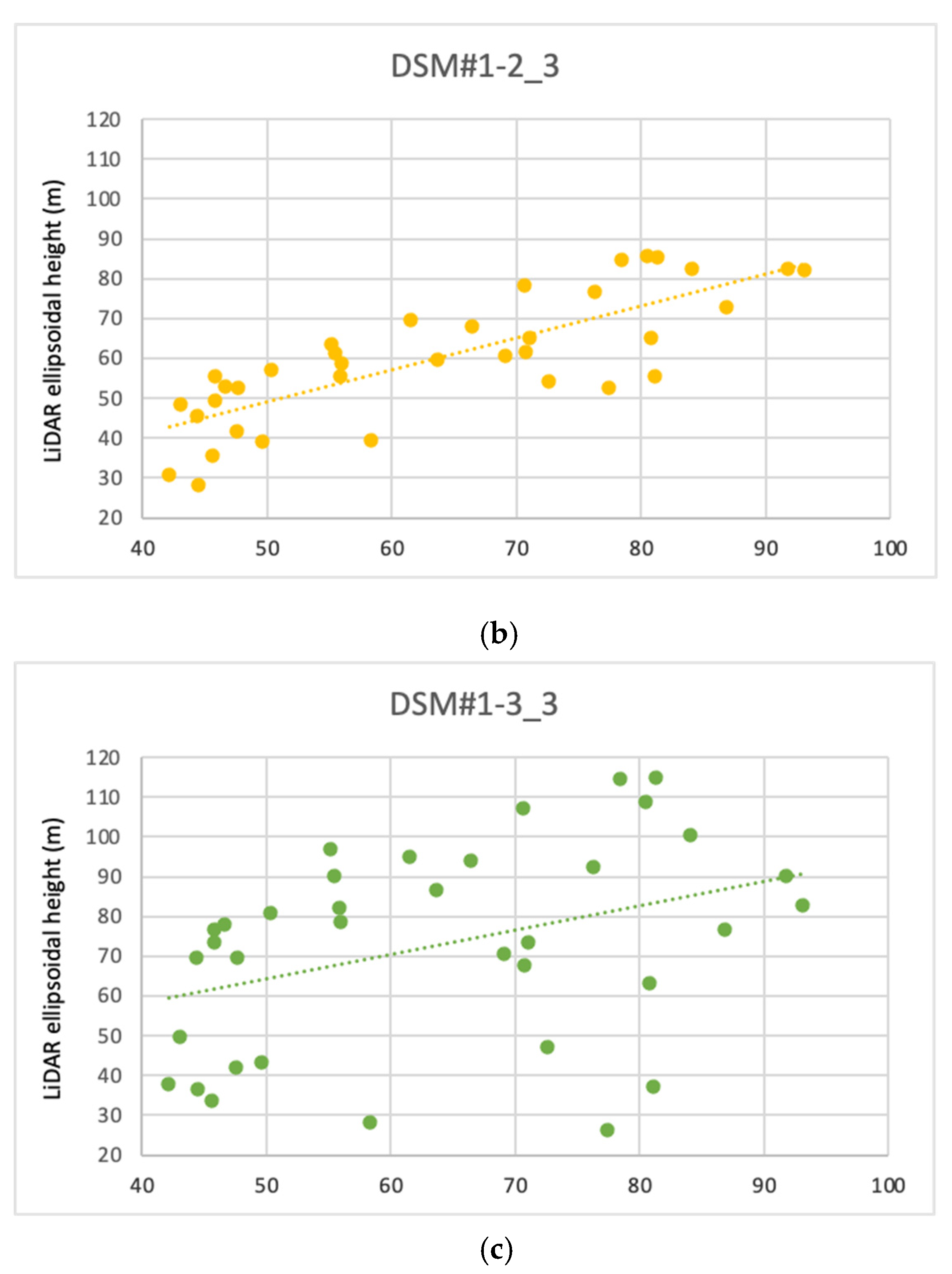
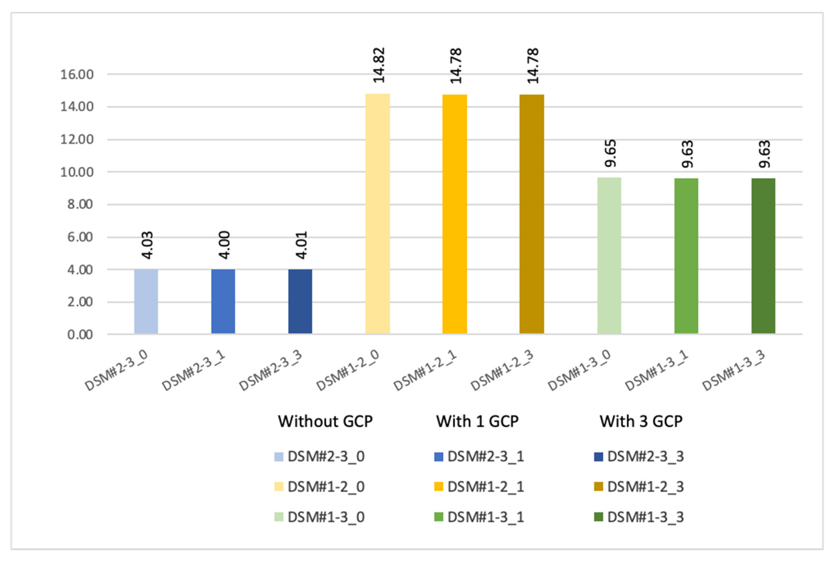
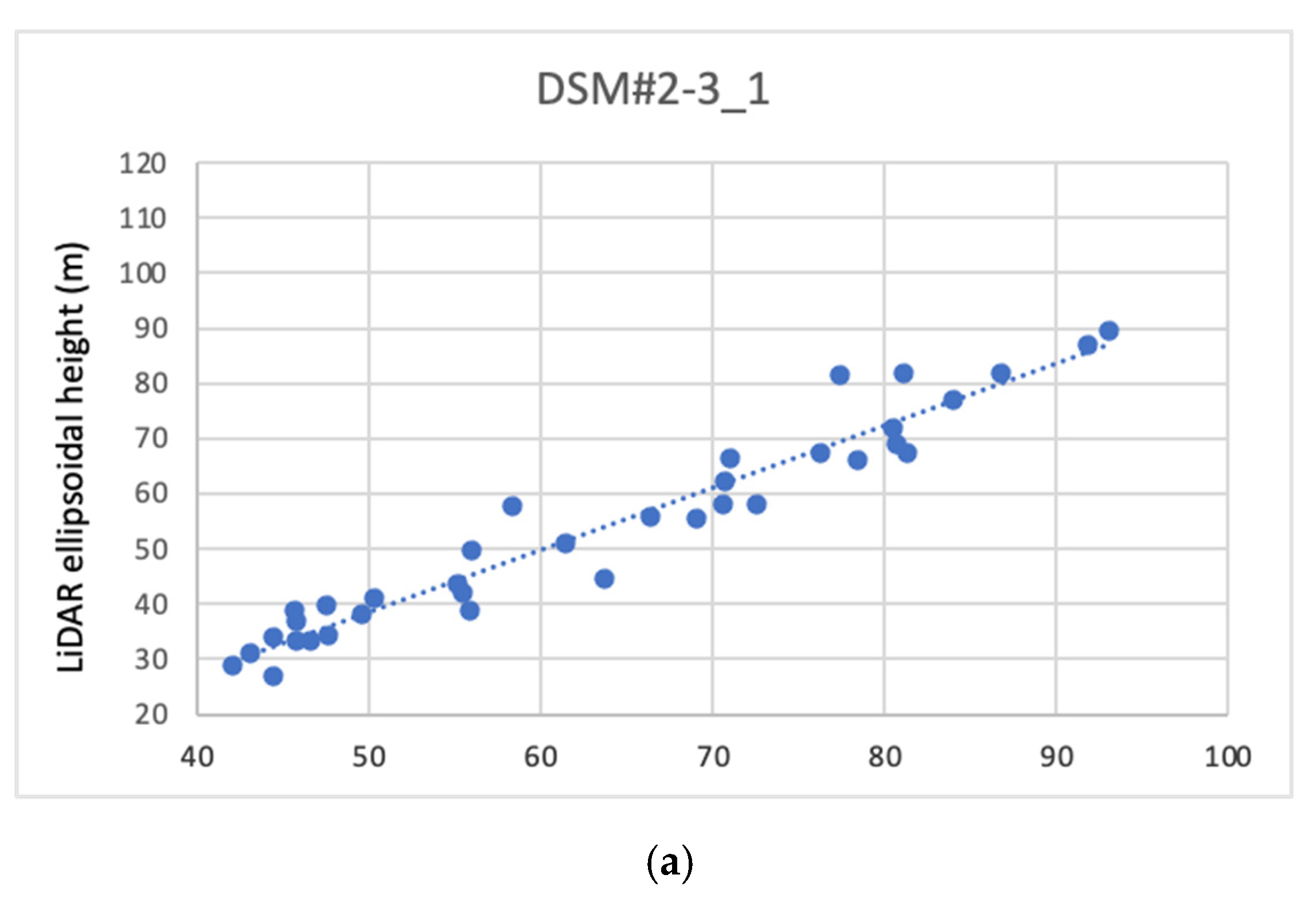
3.1.1. Global Evaluation

The results of the overall DSM evaluation showed a slight increase in the overall accuracy of the DSMs with the addition of GCPs (Figure 6). Thus, without GCP, with 1 GCP, and with 3 GCPs, the results were 4.03 m, 4 m, and 4.01 m for DSM#2–3 (Figure 6 and Figure 7a). DSM#1–2 and DSM#1–3 increased their accuracy by 0.04 m and 0.02 m, respectively, as soon as a GCP was added (Figure 6 and Figure 7b,c). However, image pairs #1–#2 and #1–#3 gave unsatisfactory results compared to image pair #2–#3.

Figure 6. Bar plot of the root mean square error from Pleiades–1 DSM computed by pairs without, with 1, or with 3 ground control points.

Figure 7. Comparison of ellipsoidal height of the LiDAR dataset and the three best digital surface models: DSM#2–3_1 (a), DSM#1–2_3 (b) and DSM#1–3_3 (c).

At the global scale, the analysis of the three best DSMs (DSM#2–3_1, DSM#1–2_3, and DSM#1–3_3) can be compared to the validation points that were extracted from the LiDAR–2018 (Figure 7a–c). The distribution of the DSM#2–3_1 points shows a low dispersion and therefore a positive correlation between the LiDAR–2018 dataset and DSM#2–3_1 (Figure 7a). The DSM#1–3_3 appeared to be sparsely correlated to the LiDAR–2018 dataset.

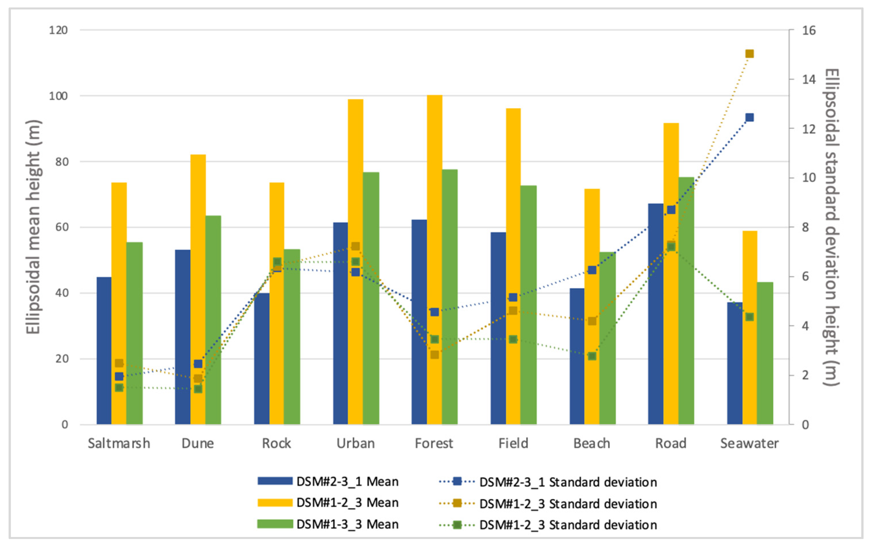
3.1.2. Class Level DSM Evaluation

The analysis of the DSM results from the Pleiades–1 images can also be examined at the class level (Figure 8) on the sub–study site. Based on the validation polygons from the classes, each DSM was evaluated.

Figure 8. Ellipsoidal mean and standard deviation height at the class level on the sub–study site from the three best digital surface models.

Depending on the ecosystem, the mean heights between the DSMs within the same class can vary. This is the case for almost all of the classes if the three DSMs are compared to each other.

However, when DSM#2–3_1 and DSM#1–3_3 are compared to each other (due to their performance at the landscape scale), the mean differences in heights were: +10.35 m, +10.22 m, +13.16 m, +15.24 m, +15.11 m, +13.95 m, +10.83 m, +7.71, and +6.15 m for the salt marsh, dune, rock, urban, forest, beach, road, and seawater classes, respectively.

3.2. Morphometric Derivatives

Four main morphometric by–products were calculated:

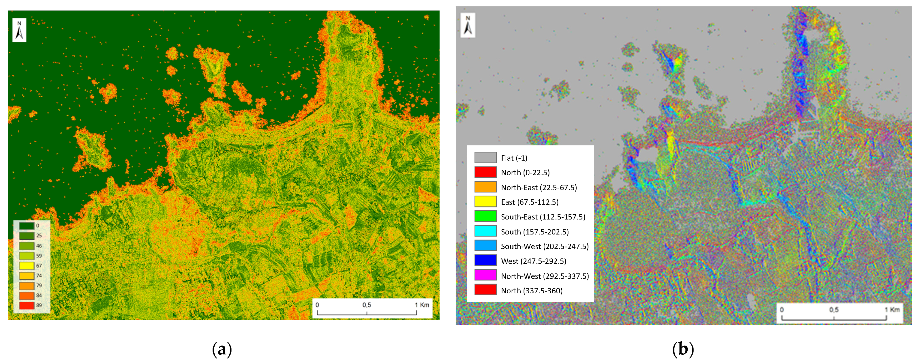
• The slope values ranged from 0 to 89°, with 0° corresponding to a flat surface such as the seawater or flatland (in green) and 89° corresponding to a steep cliff (in red in Figure 9a).
  

  Figure 9. Morphometric variables derived form the best Pleiades–1 DSM#2–3_1: slope in degrees (a); aspect (b); topographic position index, (TPI) (c); TPI–based landform classification (d).
• The aspect is categorized in 10 classes from 0 to 360°, according to the main cardinal points (north, south, east, west; Figure 9b). A value of −1 corresponds to flat areas such as those for seawater.
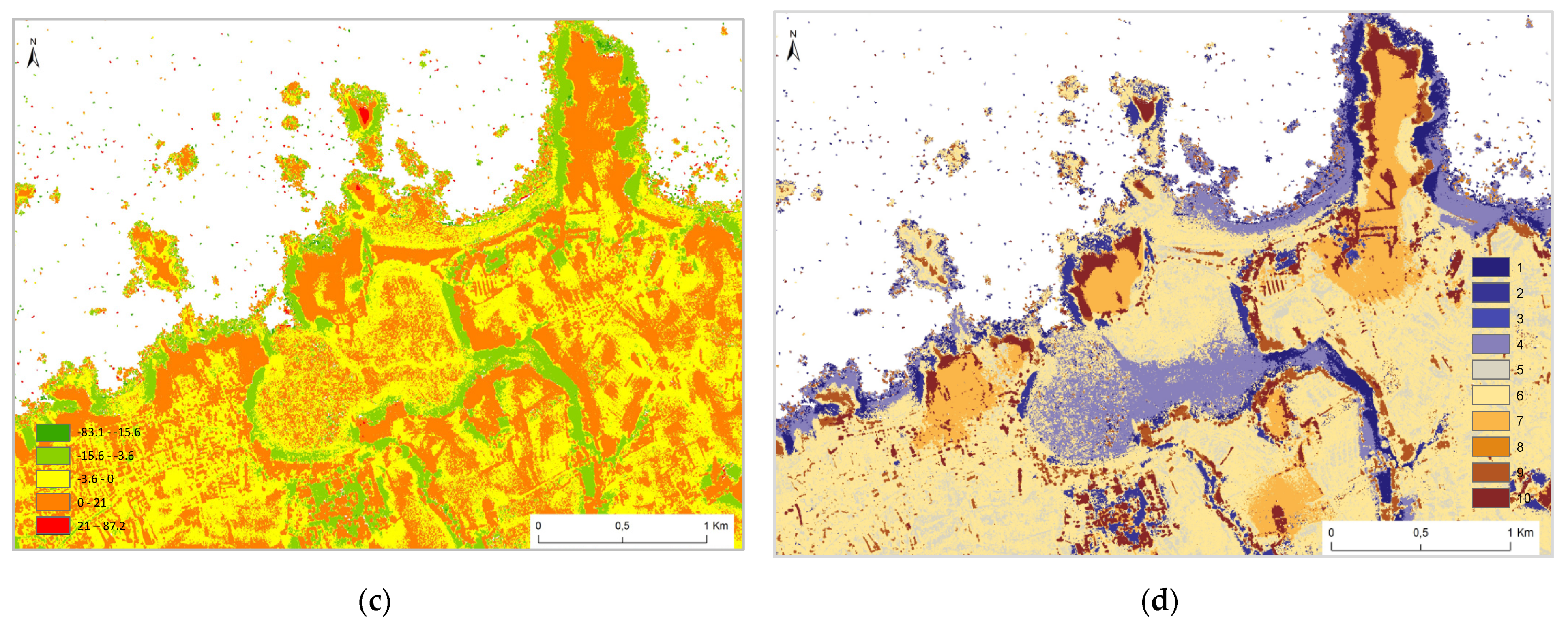
• TPI is the third morphometric contributor (Figure 9c).
• Finally, TPILC (Figure 9d) groups the landscapes into 10 classes (1 to 10).

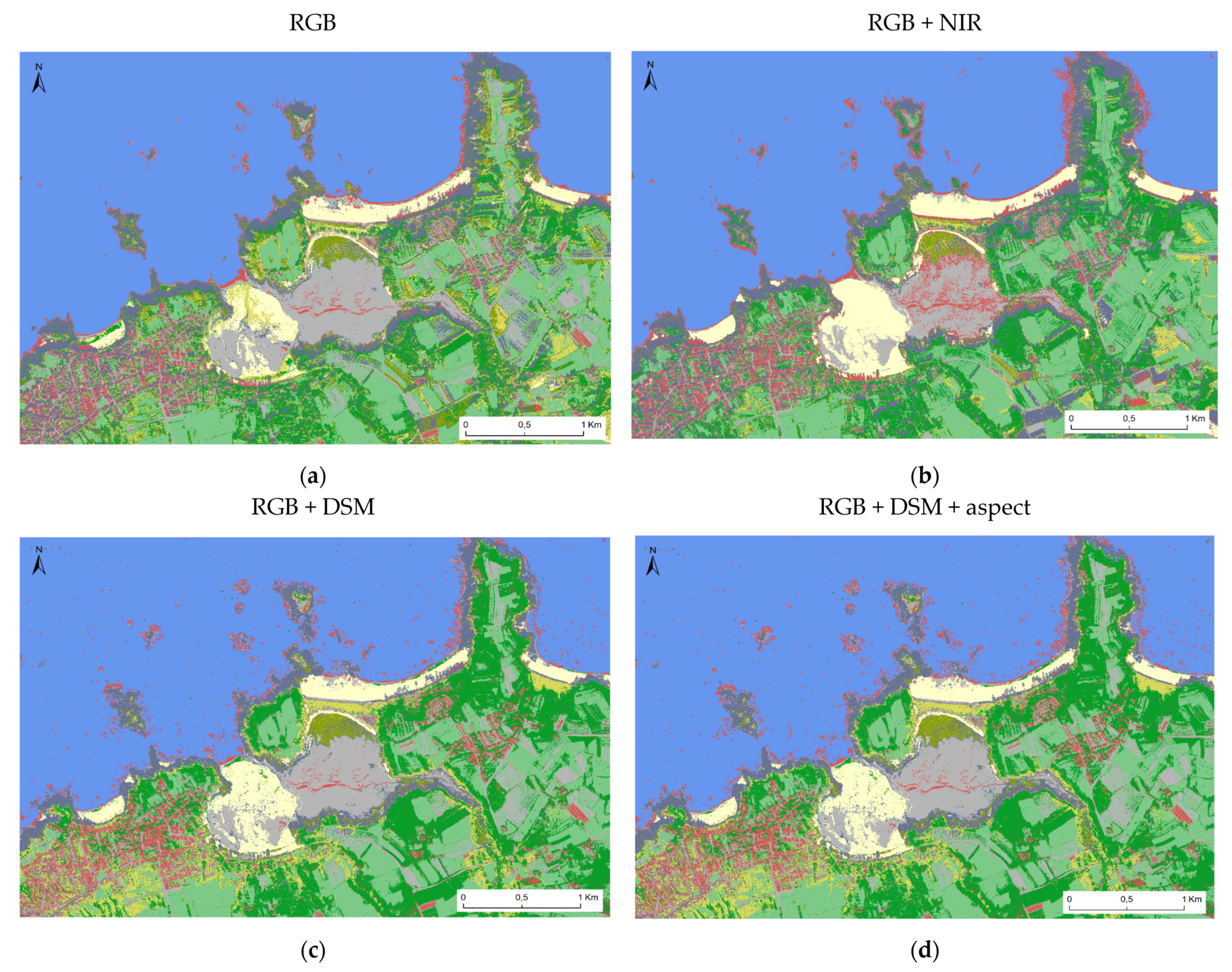
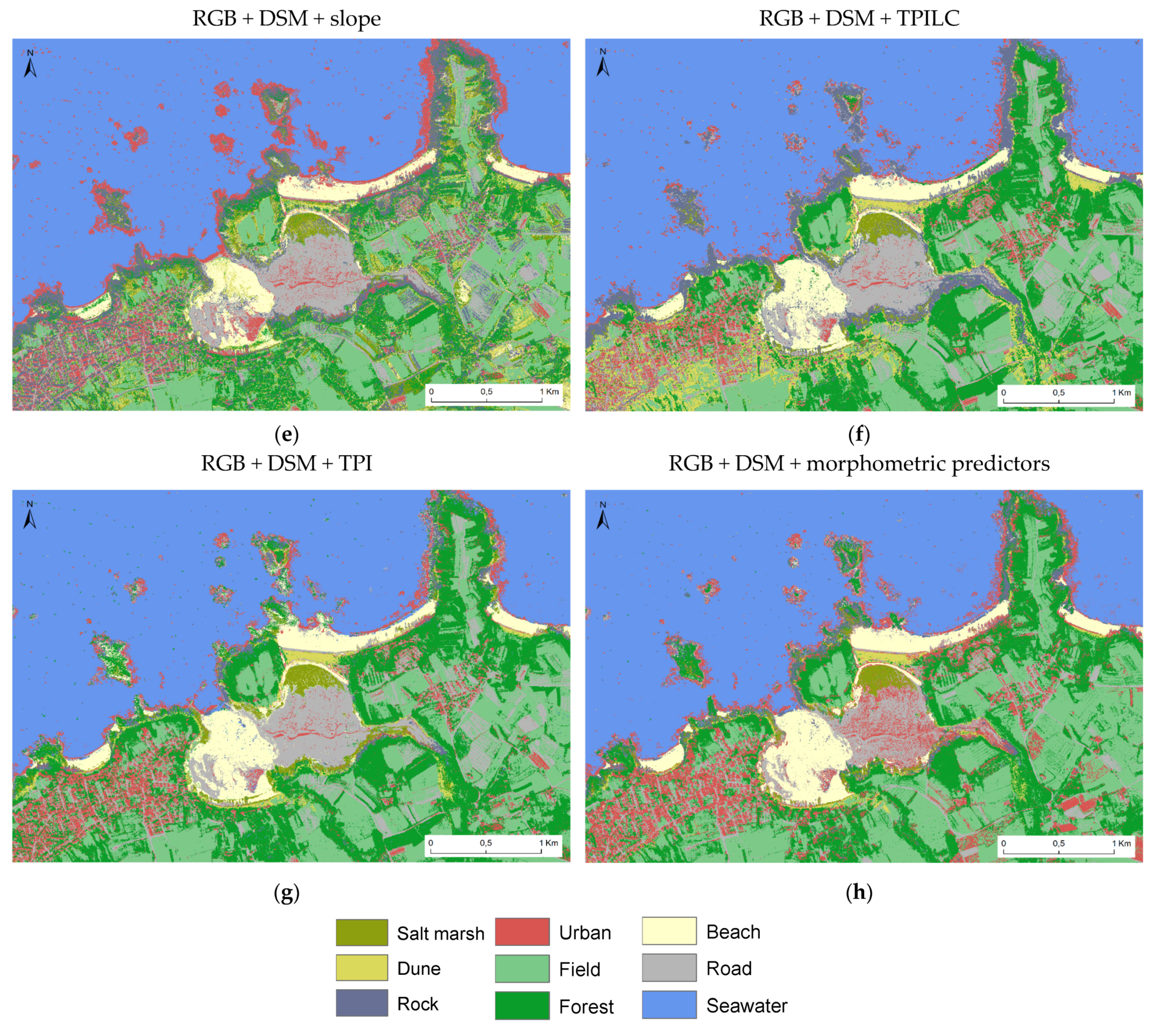
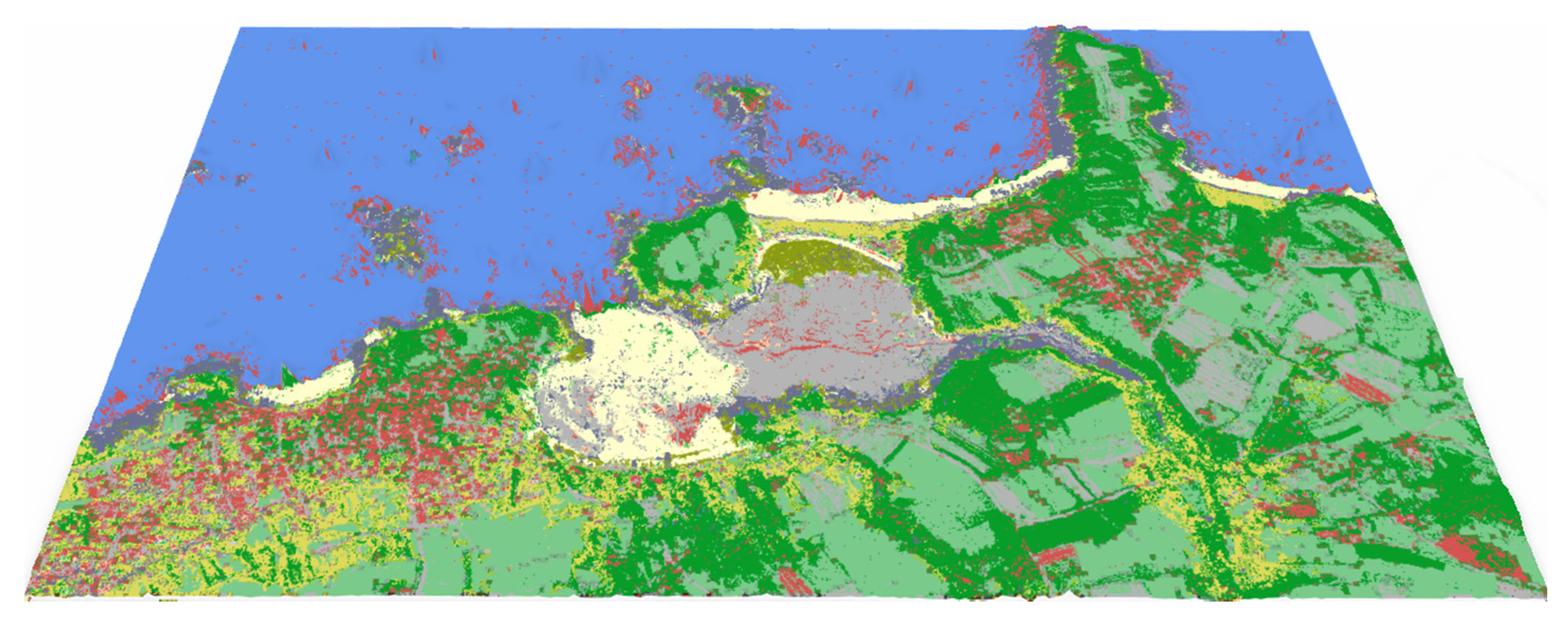
3.3. Pixel–Based Classification

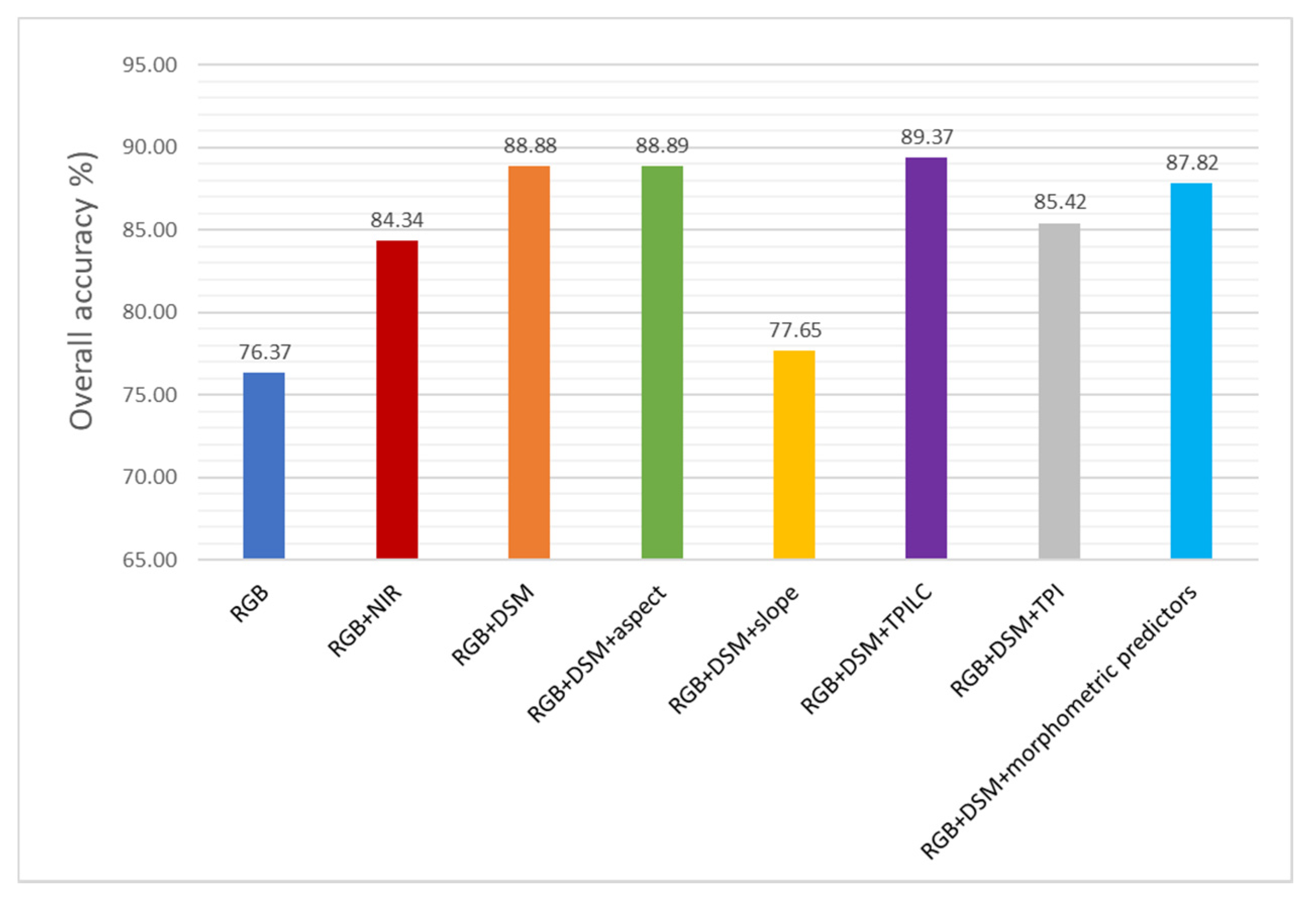
3.3.1. Overall Accuracy at the Landscape Scale

At the landscape scale, each band combination was assessed. To test individual contribution, the RGB spectral composite was used as a basis, achieving an OA of 76.37% (Figure 10).

Figure 10. Overall accuracy of the eight classifications performed with the maximum likelihood classifier.

The NIR band was also tested and obtained a score of 84.34% combined with the RGB.

Thus, in addition to the RGB, the DSM significantly enhanced the OA by +12.51%, but RGB + DSM + slope decreased the score (−11.23%) compared to the RGB + DSM combination (Figure 10).

The morphometric predictor combinations provided a strong contribution to the classification, with +9.05%, +11.45%, and +12.52% for the RGB + DSM + TPI and RGB + DSM + morphometric predictors and for RGB + DSM + aspect, respectively.

Finally, the best combination was the TPILC predictor combined with RGB + DSM, with a classification score of 89.37%, namely an augmentation of +13%.

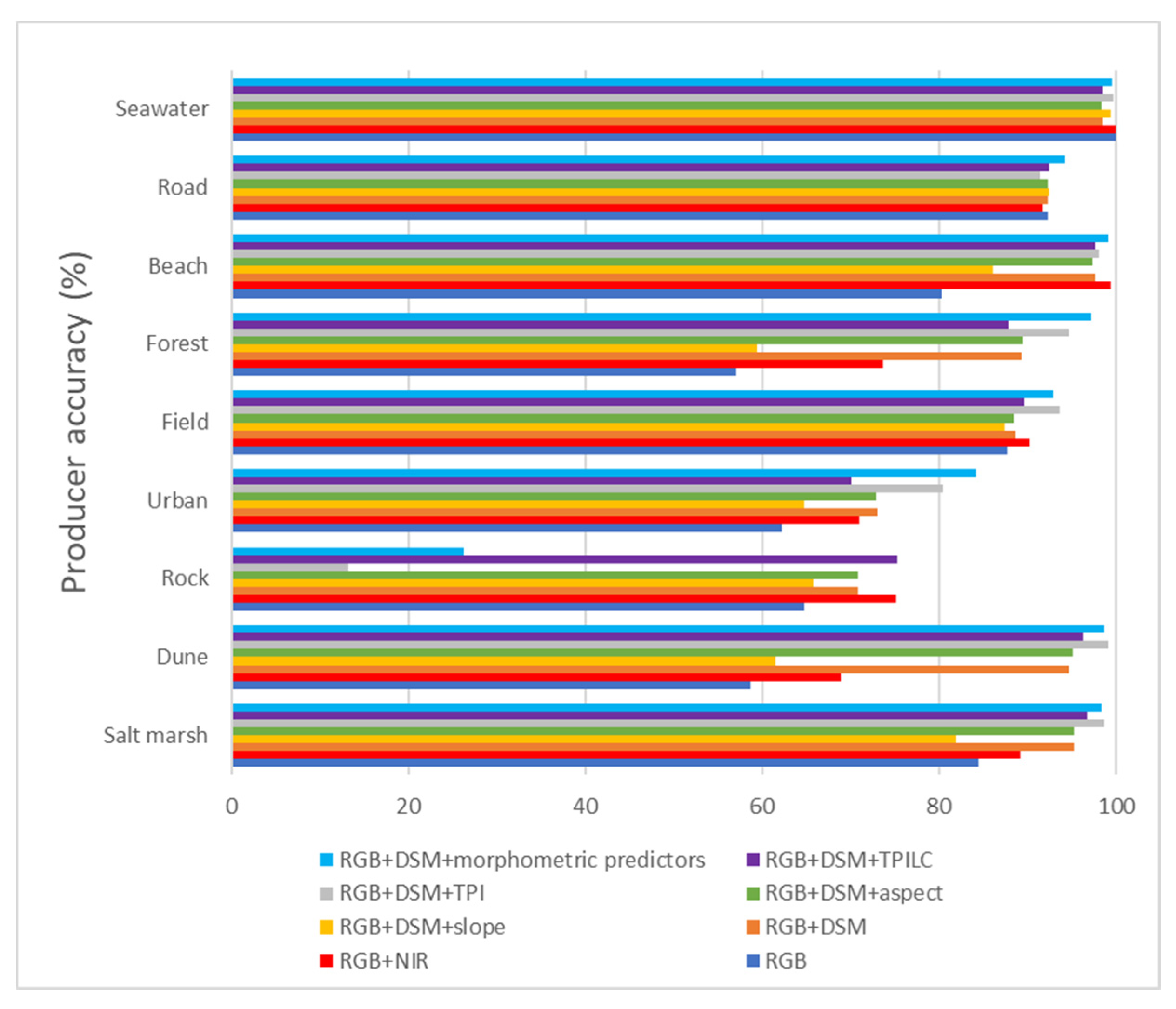
3.3.2. Evaluation at the Class Level

The analysis of the confusion matrix of each morphometric predictor added to the basic RGB highlights a heterogeneity between the classes (Table 3, Figure 11 and Figure 12).

Table 3. Producer accuracy (in %) from confusion matrix using the maximum likelihood classifier for the salt marsh, dune, rock, urban, field, forest, beach, road, and seawater classes.

	Salt Marsh	Dune	Rock	Urban	Field	Forest	Beach	Road	Seawater
RGB	84.47	58.67	64.8	62.27	87.67	57	80.27	92.27	100
RGB + NIR	89.13	68.93	75.07	71	90.27	73.67	99.4	91.67	100
RGB + DSM	95.2	94.67	70.8	73	88.6	89.27	97.67	92.33	98.47
RGB + DSM + slope	82	61.47	65.8	64.73	87.47	59.47	86.13	92.47	99.4
RGB + DSM + aspect	95.2	95.13	70.8	72.93	88.4	89.53	97.33	92.33	98.4
RGB + DSM + TPI	98.6	99.07	13.27	80.4	93.6	94.6	98.07	91.47	99.73
RGB + DSM + TPILC	96.67	96.27	75.27	70.13	89.67	87.93	97.6	92.4	98.47
RGB + DSM + morphometric predictors	98.33	98.67	26.33	84.13	92.93	97.2	99.13	94.2	99.53

Figure 11. Bar plot of the producer accuracy of the morphometric predictor on the basis RGB at the class level (salt marsh, dune, rock, field, forest, beach, road, and seawater).

Figure 12. Coastal mapping classification at the class level computed with the maximum likelihood classifier: Basis RGB (a); RGB + NIR (b); RGB + DSM (c); RGB + DSM + slope (d); RGB + DSM + aspect (e); RGB + DSM + TPI (f); RGB + DSM + TPILC (g); RGB + DSM + morphometric predictors (h).

Thus, the urban class obtained the worst results with the RGB and increased in terms of classification performance when another predictor was added. The slope predictor increased by 2.46. The addition of a morphometric predictor allowed the 70.13% of classification performance to increase until the threshold of 84.13% as reached with the combination RGB + DSM + morphometric predictor. The NIR predictor holds up reasonably, achieving a score of with 71% (Table 3, Figure 11 and Figure 12).

The trend for the forest class seems to be the same as the trend observed for the urban class. The slope provides a modest contribution of 2.47%, followed by the NIR predictor with a contribution of 16.67%, and then by the DSM contribution with a contribution of 32.27%. When added to the RGB + DSM, morphometric predictors aspect, TPILC, TPI, and the entire combination obtain values of +30.93%, +30.97%, +37.6%, and +40.2%, respectively.

The salt marsh, beach, and dune classes increased in classification accuracy when a morphometric variable was added to the reference RGB: +10.73%, +17.4%, and +36%, respectively with the RGB + DSM combination until the addition of TPI variable at 98.6% and 99.07% for the salt marsh and dune classes. The beach class obtained the best result with RGB + NIR, achieving results of 99.4%. In contrast to the salt marsh and beach classes, the rock class performed worst, with 13.27% and 26.33% with the RGB + TPI combinations and the complete combination of morphometric variables added to the RGB, respectively.

The road class obtained linear classification scores between 91.47% for RGB + DSM + TPI and 94.2% for the RGB + DSM + morphometric predictors.

The field class follows a slightly different pattern than the other classes since the worst result, which was still very acceptable, is achieved by the combination RGB + DSM + slope, with a score of 86.47%. The RGB combination increased the classification performance by only +0.2% and +0.93% for the RGB + DSM + aspect and +1.13% for the RGB + DSM combination. The RGB + DSM + TPILC, RGB + NIR, and RGB + DSM + morphometric predictors increased the classification performance by +2.2%, 2.8%, and +5.46%. The best combination for the field class was obtained by RGB + DSM + TPI, with a score of 93.6%.

The seawater class achieved high scores of almost 100% PA, regardless of the predictor (Table 3, Figure 11 and Figure 12).

4. Discussion

4.1. Pleiades–1 Digital Surface Model

4.1.1. The Intersection Angle as a Key Determinant

At the global scale, nine DSM were computed via RSP from three Pleiades–1 satellite images captured at three different angles of incidence: 16.41° for image #1, 15.35° for image #2, and 16.05° for image #3 (Figure 2a and Table 1). DSM#2–3_1, which was derived from the stereo reconstruction of images #2 and #3 outperformed, the other DSMs. According to the results of the satellite photogrammetry, reconstructions with the closest intersection angles (5.13°) produced better point–measurement accuracy compared to the the 2018–LiDAR altimetric reference. Another answer can also be provided by focusing on the solar angle [21]. Moreover, close or near–similar intersection angles increase the risk of “hidden sides” because of their proximity [22,23].

However, many studies have shown interest in using tri–stereo satellite images to benefit, when possible, from a nadir view [24]. The benefit of such a tri–stereo enables a reduction in the shadows that are created by trees or buildings. This approach is highly valued by urban planners, as it limits the risk of shadows and hidden areas [25].

As for photogrammetric reconstructions from UAV images, a deficient RMSE could be explained by reconstruction artifacts related to the algorithm or to the images themselves [26].

4.1.2. Ground Control Point Effect

At a more local scale, three scenarios can explain the results that were obtained. The first is the number of GCP that were extracted from the 2018–LiDAR as calibration points for our topographic models. The tests that were performed without GCP, with one, or with three GCP, showed that when we added GCP points, the model is more accurate [27]. However, The RPC files that were delivered with the Pleiades–1 images could be more powerful. The RPC files integrate all of the parameters that are related to the photographs in order to correct for the satellite images. This approach could be investigated in a future study.

4.1.3. Information Reflected by the LiDAR Wavelengths

Two laser sensors were used for the whole LiDAR dataset: a mixed topo–bathymetric laser in the NIR and green spectra, and a stronger bathymetric laser in the green spectrum, which was specifically used for deeper areas. Depending on the nature (albedo) of the coastal habitat, the wavelength that is used by the LiDAR does not return the same information, being more or less reflected. Thus, the reflectance in the NIR is strong for eco–geo–systems with high chlorophyll dominance, and conversely, it is fully absorbed by habitats with a high water content, such as seawater, for example [28].

The density of the LiDAR points may also play a crucial role. The intertidal and coastal land area is denser in a number of points per square meter than marine area (deep water area) is. The detection of features such as trees is easy when the density of measured points is high [29].

4.2. Topographic Contribution to Habitat Classification

At the landscape scale, the contribution of the morphometric predictors surpassed the classification performance. Although the basic RGB performs well, as soon as morphometric predictors are added, the OA increases (from +1.28% to +13%). The positive effect of the slope raster and its by–products on the landscape classification were evidenced in several studies based on satellite sensors [30] as well as in UAV studies [31]. The classification test with the addition of the NIR band showed the relevance of a classification with morphometric variables. Indeed, when these variables were added to the RGB, the classification performance on the coastal fringe increased considerably contrary to the multispectral RGB + NIR combination without any other predictors.

At the ecosystem class level, the morphometric predictors produced different results depending on the coastal habitat type. For example, the topographic variables provided successful results for salt marshes. This particular ecosystem is located in a geographical area that is sheltered from strong prevailing marine currents. Coastal erosion has minimal or no impact on the meadows, allowing the different plant species to grow.

5. Conclusions

This research study on satellite photogrammetry with Pleiades–1 tri–stereo images is meaningful for the classification of coastal landscapes at VHR, especially in the context of climate change and increasing anthropic pressure on the coastal fringe.

Three pairs of Pleiades–1 panchromatic images at the 0.5 m pixel size were tested for DSM generation, and nine DSM were evaluated from 36 2018 LiDAR validation points.

The best DSM was derived from images #2 and #3 (DSM#2–3_1), which featured, respectively, with incidence angles of 15.35° and 16.05° and an intersection angle of 5.13°. From this new DSM, four morphometric by–products were calculated: slope, aspect, topographic position index (TPI), and TPI–based landform classification (TPILC).

A pixel–based classifier, the probabilistic maximum likelihood, was applied to the 0.5 m pansharpened RGB images, which initially had a pixel side of 2 m. Nine classes (dune, salt marsh, rock, urban, field, forest, beach, road, and seawater) were examined to map the study site (Figure 13). The best combination of morphometric predictors provided a gain of 13% in the OA, reaching 89.37%, when added to the RGB + DSM. These findings will help scientists and managers who tasked with the coastal risks at VHR.

Figure 13. Best map classification draped over the best digital surface model.

In a study that will be published in the near future, photogrammetric reconstruction from a Pleiades–Neo panchromatic triplet at the 0.30 m spatial resolution will be evaluated, given that this new sensor benefits from six bands (purple, blue, green, red, red edge, NIR), meaning that it has two additional bands compared to Pleiades–1. Moreover, the purple band will be interesting to investigate for the sake of bathymetry extraction.

References

- Zhu, Z.; Lu, L.; Zhang, W.; Liu, W. AR6 Climate Change 2021: The Physical Science Basis; IPCC: Geneva, Switzerland, 2021. [Google Scholar]
- Mousavi, M.E.; Irish, J.L.; Frey, A.E.; Olivera, F.; Edge, B.L. Global warming and hurricanes: The potential impact of hurricane intensification and sea level rise on coastal flooding. Clim. Chang. 2010, 104, 575–597. [Google Scholar] [CrossRef]
- Collin, A.; James, D.; Jeanson, M. Mapping Tropical Coastal Social–Ecological Systems Using Unmanned Airborne Vehicle (UAV). In Marine Geological and Biological Habitat Mapping Geohab; 2019; Available online: https://hal.archives–ouvertes.fr/hal–02134739/document (accessed on 23 October 2021).
- Zanutta, A.; Lambertini, A.; Vittuari, L. UAV Photogrammetry and Ground Surveys as a Mapping Tool for Quickly Monitoring Shoreline and Beach Changes. J. Mar. Sci. Eng. 2020, 8, 52. [Google Scholar] [CrossRef] [Green Version]
- James, D.; Collin, A.; Mury, A.; Letard, M.; Guillot, B. UAV Multispectral Optical Contribution to Coastal 3D Modelling. In Proceedings of the 2021 IEEE International Geoscience and Remote Sensing Symposium IGARSS, Brussels, Belgium, 11–16 July 2021; pp. 7951–7954. [Google Scholar]
- Collin, A.; Dubois, S.; Ramambason, C.; Etienne, S. Very high–resolution mapping of emerging biogenic reefs using airborne optical imagery and neural network: The honeycomb worm (Sabellaria alveolata) case study. Int. J. Remote Sens. 2018, 39, 5660–5675. [Google Scholar] [CrossRef] [Green Version]
- Ishiguro, S.; Yamada, K.; Yamakita, T.; Yamano, H.; Oguma, H.; Matsunaga, T. Classification of Seagrass Beds by Coupling Airborne LiDAR Bathymetry Data and Digital Aerial Photographs. Landsc. Ecol. Asian Cult. 2016, 59–70. [Google Scholar] [CrossRef]
- Collin, A.M.; Andel, M.; James, D.; Claudet, J. The superspectral/hyperspatial worldview–3 as the link between spaceborne hyperspectral and airborne hyperspatial sensors: The case study of the complex tropical coast. ISPRS Int. Arch. Photogramm. Remote Sens. Spat. Inf. Sci. 2019, XLII–2/W13, 1849–1854. [Google Scholar] [CrossRef] [Green Version]
- Collin, A.; Archambault, P.; Planes, S. Bridging Ridge–to–Reef Patches: Seamless Classification of the Coast Using Very High Resolution Satellite. Remote Sens. 2013, 5, 3583–3610. [Google Scholar] [CrossRef] [Green Version]
- Satellite Imaging Corporation. Available online: https://www.satimagingcorp.com/satellite–sensors/ (accessed on 30 October 2021).
- James, D.; Collin, A.; Mury, A.; Costa, S. Very high resolution land use and land cover mapping using pleiades–1 stereo im–agery and machine learning. Int. Arch. Photogramm. Remote Sens. Spat. Inf. Sci. 2020, 43, 675–682. [Google Scholar] [CrossRef]
- James, D.; Collin, A.; Mury, A.; Letard, M. Enhancing uav coastal mapping using infrared pansharpening. ISPRS Int. Arch. Photogramm. Remote Sens. Spat. Inf. Sci. 2021, XLIII–B3–2, 257–264. [Google Scholar] [CrossRef]
- Archer, A.W. World’s highest tides: Hypertidal coastal systems in North America, South America and Europe. Sediment. Geol. 2013, 284, 1–25. [Google Scholar] [CrossRef]
- Airbus. Available online: https://www.intelligence–airbusds.com/imagery/constellation/pleiades/ (accessed on 30 October 2021).
- Qin, R. Rpc stereo processor (rsp)—A software package for digital surface model and orthophoto generation from satellite stereo imagery. ISPRS Ann. Photogramm. Remote Sens. Spat. Inf. Sci. 2016, 3, 77. [Google Scholar] [CrossRef] [Green Version]
- Saga Gis. Available online: http://www.saga–gis.org/ (accessed on 17 October 2021).
- Weiss, A.D. Topographic position and landforms analysis. In Proceedings of the Poster Presentation, ESRI Users Conference, San Diego, CA, USA, 9–13 July 2001. [Google Scholar]
- Guisan, A.; Weiss, S.B.; Weiss, A.D. GLM versus CCA spatial modeling of plant species distribution. Plant Ecol. 1999, 143, 107–122. [Google Scholar] [CrossRef]
- Harris Geospatial. Available online: https://www.l3harrisgeospatial.com/Software–Technology/ENVI (accessed on 21 July 2021).
- Story, M.; Congalton, R.G. Accuracy assessment: A user’s perspective. Photogramm. Eng. Remote Sens. 1986, 52, 397–399. [Google Scholar]
- Qui, R. A Critical Analysis of Satellite Stereo Pairs for Digital Surface Model Generation and A Matching Quality Prediction Model. ISPRS J. Photogramm. Remote Sens. 2019, 154, 139–150. [Google Scholar]
- Poli, D.; Remondino, F.; Angiuli, E.; Agugiaro, G. Evaluation of pleiades–1a triplet on trento testfield. ISPRS Int. Arch. Photogramm. Remote Sens. Spat. Inf. Sci. 2013, XL–1/W1, 287–292. [Google Scholar] [CrossRef] [Green Version]
- Collin, A.; Hench, J.L.; Pastol, Y.; Planes, S.; Thiault, L.; Schmitt, R.J.; Holbrook, S.J.; Davies, N.; Troyer, M. High resolution topobathymetry using a Pleiades–1 triplet: Moorea Island in 3D. Remote Sens. Environ. 2018, 208, 109–119. [Google Scholar] [CrossRef]
- Bernard, M.; Decluseau, D.; Gabet, L.; Nonin, P. 3D capabilities of pleiades satellite. ISPRS Int. Arch. Photogramm. Remote Sens. Spat. Inf. Sci. 2012, XXXIX–B3, 553–557. [Google Scholar] [CrossRef] [Green Version]
- Panagiotakis, E.; Chrysoulakis, N.; Charalampopoulou, V.; Poursanidis, D. Validation of Pleiades Tri–Stereo DSM in Urban Areas. ISPRS Int. J. Geo Inf. 2018, 7, 118. [Google Scholar] [CrossRef] [Green Version]
- Pichon, L.; Ducanchez, A.; Fonta, H.; Tisseyre, B. Quality of digital elevation models obtained from unmanned aerial vehicles for precision viticulture. OENO One 2016, 50, 3. [Google Scholar] [CrossRef] [Green Version]
- Rupnik, E.; Deseilligny, M.P.; Delorme, A.; Klinger, Y. Refined satellite image orientation in the free open–source photogram–metric tools Apero/Micmac. ISPRS Ann. Photogramm. Remote Sens. Spat. Inf. Sci. 2016, 3, 83. [Google Scholar] [CrossRef] [Green Version]
- Letard, M.; Collin, A.; Lague, D.; Corpetti, T.; Pastol, Y.; Ekelund, A.; Pergent, G.; Costa, S. Towards 3D Mapping of Seagrass Meadows with Topo–Bathymetric Lidar Full Waveform Processing. In Proceedings of the 2021 IEEE International Geoscience and Remote Sensing Symposium IGARSS, Brussels, Belgium, 11–16 July 2021; pp. 8069–8072. [Google Scholar] [CrossRef]
- Farid, A.; Rautenkranz, D.; Goodrich, D.C.; Marsh, S.E.; Sorooshian, S. Riparian vegetation classification from airborne laser scanning data with an emphasis on cottonwood trees. Can. J. Remote Sens. 2006, 32, 15–18. [Google Scholar] [CrossRef]
- Lee, D.G.; Shin, Y.H.; Lee, D.C. Land Cover Classification Using SegNet with Slope, Aspect, and Multidirectional Shaded Relief Images Derived from Digital Surface Model. J. Sens. 2020, 2020, 8825509. [Google Scholar] [CrossRef]
- James, D.; Collin, A.; Houet, T.; Mury, A.; Gloria, H.; Le Poulain, N. Towards Better Mapping of Seagrass Meadows using UAV Multispectral and Topographic Data. J. Coast. Res. 2020, 95, 1117–1121. [Google Scholar] [CrossRef]
Publisher’s Note: MDPI stays neutral with regard to jurisdictional claims in published maps and institutional affiliations. |
© 2022 by the authors. Licensee MDPI, Basel, Switzerland. This article is an open access article distributed under the terms and conditions of the Creative Commons Attribution (CC BY) license (https://creativecommons.org/licenses/by/4.0/).