Discrete Atomic Transform-Based Lossy Compression of Three-Channel Remote Sensing Images with Quality Control

Abstract

Lossy compression of remote sensing data has found numerous applications. Several requirements are usually imposed on methods and algorithms to be used. A large compression ratio has to be provided, introduced distortions should not lead to sufficient reduction of classification accuracy, compression has to be realized quickly enough, etc. An additional requirement could be to provide privacy of compressed data. In this paper, we show that these requirements can be easily and effectively realized by compression based on discrete atomic transform (DAT). Three-channel remote sensing (RS) images that are part of multispectral data are used as examples. It is demonstrated that the quality of images compressed by DAT can be varied and controlled by setting maximal absolute deviation. This parameter also strictly relates to more traditional metrics as root mean square error (RMSE) and peak signal-to-noise ratio (PSNR) that can be controlled. It is also shown that there are several variants of DAT having different depths. Their performances are compared from different viewpoints, and the recommendations of transform depth are given. Effects of lossy compression on three-channel image classification using the maximum likelihood (ML) approach are studied. It is shown that the total probability of correct classification remains almost the same for a wide range of distortions introduced by lossy compression, although some variations of correct classification probabilities take place for particular classes depending on peculiarities of feature distributions. Experiments are carried out for multispectral Sentinel images of different complexities.

1. Introduction

In recent years, remote sensing (RS) has found various applications [1,2,3,4], including in agriculture [5,6], forestry, catastrophe, ecological monitoring [5], land cover classification [6,7], and so on. This can be explained by several reasons. First, a great amount of useful information can be retrieved from acquired images, especially if they are high resolution and multichannel, which represents a set of component images of the same territory obtained in parallel or sequentially and co-registered [3,5,6] (using the term “multichannel”, we mean that component images can be acquired for different polarizations, wavelengths, or even by different sensors). Second, the situation with RS data value and volume becomes even more complicated because many modern RS systems can carry out frequent data collection, e.g., once a week or more frequently. Sentinel-1 and Sentinel-2 recently put into operation are examples of sensors producing such large volume multichannel RS data [7,8]. Other examples are hyperspectral data provided by different sensors [9,10,11].

Then, problems of big data arise [9,10] where efficient transmission, storage, and dissemination of RS data are several of them, alongside others relating to co-registration, filtering, and classification. In RS data transmission, storage, and dissemination, compression are helpful [12,13,14,15]. Both lossless [12,13,16] and lossy [14,15,17] approaches are intensively studied. Near-lossless methods have been designed and analyzed as well [18,19]. Lossless techniques produce undistorted data after decompression, but the compression ratio (CR) is often not large enough. Near-lossless methods allow obtaining larger values of CR, and introduced distortions are controlled (restricted) in one or another manner [20]. However, CR can be still not large enough. In turn, the lossy compression we focus on in this paper is potentially able to produce CR equal to tens and larger than one hundred [17,21]. This can be achieved by the expense of distortions where larger distortions are introduced for larger CR values. A question is what is a reasonable trade-off between an attained CR and introduced distortions [13,22,23,24,25] and how can it be reached?

An answer depends upon many factors:

(1)

Priority of requirements to compression, restrictions that can be imposed;

(2)

Criteria of compressed image quality, tasks to be solved using compressed images;

(3)

Image properties and characteristics;

(4)

Available computational resources, preference of mathematical tools that can be used as compression basis.

Consider all these factors. Compression can be used for different purposes, including reduction of data size before their downlink transferring from a sensor to a point of data reception via a limited bandwidth communication line, to store acquired images for their further use in national or local centers of RS data, and to transfer data to potential customers [13,23].

First, providing a given CR with a minimal level of distortions can be of prime importance. Then, the use of efficient spectral and spatial decorrelation transforms is needed [17,23,24], combined with modern coding techniques applied to quantized transform coefficients. Spectral decorrelation and 3D compression allow exploiting spectral redundancy of multichannel data inherent for many types of images as, e.g., multispectral and hyperspectral [25], to increase CR [24]. In this paper, we consider three-channel images combined of visible range components of Sentinel-2 images [25]. The main reason we consider separate compressions of component images with central wavelengths 492 nm (Blue), 560 nm (Green), and 665 nm (Red) of Sentinel-2 data (https://www.esa.int/Applications/Observing_the_Earth/Copernicus/Sentinel-2, accessed on 27 October 2021) is that they have the equal resolution that differs from the resolution of most other (except NIR-band) component images (in other words, we assume that Sentinel-2 images can be compressed in several groups, taking into account different resolutions in different component images, namely, 10 × 10, 20 × 20, and 60 × 60 m²). Besides, earlier, discrete atomic compression (DAC) was designed for color images (i.e., for three-channel image compression).

Second, it is possible that the main requirement is to provide the introduced losses below a given level. “Below a given level” can be described quantitatively or qualitatively. In the former case, one needs some criterion or criteria to measure the introduced distortions (see brief analysis below). In the latter case, it can be stated that, e.g., lossy compression should not lead to sufficient reduction of image classification accuracy (although even in this case “sufficient” can be described quantitatively). Here, it is worth recalling that considerable attention has been paid to the classification of lossy compressed images [17,26,27,28,29,30,31,32,33]. It has been shown that lossy compression can sometimes improve classification accuracy or, at least, the classification of compressed data provides approximately the same classification accuracy as classification of uncompressed data [34,35,36]. Thus, if compression is lossy, the procedures of providing appropriate quality of compressed data are needed [36].

Third, it is often desired to carry out compression quickly enough. In this sense, it is not reasonable to employ iterative procedures, especially if the number of iterations is random and depends on many factors. It is worth applying transforms that can be easily implemented and have fast algorithms, can be parallelized, and so on [12]. This explains why most efficient methods are based on discrete cosine transform and wavelets [36,37,38,39]. Here, we consider lossy compression based on discrete atomic transform (DAT) [40,41] where atomic functions are a specific kind of compactly supported smooth functions. As it will be shown below, DAT has a set of properties that are useful in the lossy compression of multichannel images.

Fourth, there can also be other important requirements. They can relate to the visual quality of compressed images [26], the necessity to follow some standards, etc. One of the specific requirements could be the security and privacy of compressed data [42,43]. There are many approaches to providing security and privacy of images in general and RS data in particular [44,45,46]. Currently, we concentrate on the problem of unauthorized viewing of image content. Usually, a processing procedure, which provides both compression and content protection, can be constructed as follows: image is compressed and afterward encrypted. This approach requires considerable additional computational resources, especially if a great number of digital images is processed. Another way is to apply a combination of some special image transform at the first step (for example, scramble technique [46]) with further data compressing. In this case, the following questions arise: (1) what compression efficiency is provided? (2) is it possible to reconstruct an image correctly if a lossy compression algorithm is applied? It has been recently shown that privacy of images compressed by DAT [47] can be provided practically without increasing the size of compressed files (actually, protection is integrated into compression). This is one of its obvious advantages that will be discussed in this paper in more detail.

As has been mentioned above, criteria of compressed image quality and tasks to be solved using compressed images describe the efficiency of compression and applicability of compressed data for further use. The maximal absolute deviation is often used in characterizing near-lossless compression [19]. Root mean square error (RMSE), mean square error (MSE) and peak signal-to-noise ratio (PSNR) are conventional metrics used in lossy image compression [13,26]. Different visual quality metrics are applied as well [48,49,50]. Criteria typical for image classification (a total (aggregate) probability of correct classification, probabilities of correct classification for particular classes, confusion matrices) are worth using if RS data classification is the final task of image processing [51]. There is a certain correlation between all these criteria, but they are not strictly established yet [52]. Because of this, it is worth carrying out studies for establishing such correlations. Note that correlations between aforementioned probabilities and compressed image quality characterized by maximal absolute deviation (MAD) or PSNR depend upon a classifier used [36,53,54]. In this paper, we employ the maximum likelihood (ML) method [25,53,54]. This method has shown itself to be efficient for classifying multichannel data [53,54,55], its efficiency is comparable to the efficiency of neural network classifier [36].

We have stated above that image properties and characteristics influence CR and coder performance. For simpler structure images, the introduced losses are usually smaller than for complex structure images for the same CR where image complexity can be characterized by, e.g., entropy (a larger entropy relates to more complex structure images). This means that compression should be analyzed for images of different complexity and, desirably, of natural scenes. Besides, noise present in images can influence image compression. First, noisy images are compressed worse than the corresponding noise-free images [25]. Second, if images are noisy, this should be taken into account in compression performance analysis and coder parameter setting [18,56]. Since component images in the visible range of multispectral Sentinel-2 data have a high signal-to-noise ratio (that corresponds to noise invisibility in case of image visual inspection), we further consider these images noise-free.

We assume that available computational resources, preference of mathematical tools to be used for compression are not of prime importance. Meanwhile, we can state that the DAT-based compression analyzed below possesses high computational efficiency [57].

Aggregating all these, we concentrate on the following:

• DAT is used as the basis of compression and we are interested in the analysis of its performance since it is rather fast, allows providing privacy of data, and has some other advantages [40,41,47,57];
• It is worth investigating how compression characteristics of DAT can be varied (adapted to practical tasks) and how the main criteria characterizing compression performance are inter-related;
• We are interested in how the DAT-based compression influences classification accuracy and, for this purpose, consider the classification of three-channel Sentinel-2 data using the ML method.

Thus, the goal of this paper is to carry out a thorough analysis of DAT application for compressing and further analysis of multichannel RS images using three-channel Sentinel-2 data. The main contributions of the paper are the following. First, we analyze and show what versions of DAT are the most attractive (preferable) for the considered application. Second, we analyze and propose ways to control distortions introduced by DAC. Third, we study how DAC influences the classification accuracy of RS data and show what parameter values have to be set to avoid sufficient degradation of classification characteristics.

The paper structure is the following. Section 2 considers DAT-based compression and its variants, basics of privacy providing. In Section 3, dependencies between the main parameters and criteria of DAT compression are investigated. Section 4 describes the used classifier and its training for two test images. Section 5 provides the results of experiments (classification) for the real-life three-channel image. A brief discussion is given in Section 6. Finally, the conclusions follow.

2. DAT-Based Compression and Its Properties

Below, we describe the discrete atomic compression that is the DAT-based image compression algorithm. Then, we consider the procedure of DAT, which is its core, and quality control mechanism.

2.1. Discrete Atomic Compression

In the algorithm DAC, the following classic lossy image compression approach is used: preprocessing → discrete transform → quantization → encoding. The application of DAC to full-color digital image processing is shown in Figure 1. In this case, the input is RGB-matrix. At the first step, luma (Y) and chroma (Cr, Cb) components are obtained. Further, each matrix Y, Cr, and Cb is processed separately. The procedure DAT is applied to them and matrices Ω^[Y], Ω^[Cr], Ω^[Cb] of DAT coefficients are computed. Next, elements of these matrices are quantized (further, we consider this process in more detail). Finally, quantized DAT-coefficients are encoded using a lossless compression algorithm. The range of most of these values is small. Moreover, depending on quantization coefficients choice, a significant part of them is equal to zero. A combination of the features described provides effective compression by such algorithms, as Huffman codes, which are often used in combination with run-length encoding, as well as arithmetic coding (AC) [55]. Consider this in more detail.

In this research, we apply the algorithm AC to compress bit streams obtained from quantized DAT-coefficients. Different ways to transform data into bitstream can be used. For example, the special bit planes bypass is applied in JPEG2000 [37]. In the current research, we use an approach that is based on Golomb coding [58]. Our proposition is to apply the following bitstream assignment: 0 ↔ 0, 1 ↔ 10, −1 ↔ 110, 2 ↔ 1110, −2 ↔ 11110, etc. In general, the code for 0 is 0, the code for positive k is the sequence of 2k−1 bits equal to 1 and end-bit 0, the code for negative −k is the sequence of 2k bits equal to 1 and end-bit 0. For example, a binary stream of the sequence {0, 3, 4, −1, −2, 1, 0, 0, 2} is 0111110111111101101111010001110. In addition, we use row-by-row scanning of the coded blocks. The choice of such a scan is based primarily on performance reasons, namely, on the principle of locality, which allows significant speeding up the data processing by effectively using the features of the memory architecture [59]. Of course, there may be another way to bypass the blocks, which might provide better compression efficiency.

The process of reconstructing a compressed image is carried out in the reverse order to that shown in Figure 1.

We note that the algorithm DAC can be used to compress grayscale digital images. In this case, the preprocessing step is skipped, and DAT is applied directly to the matrix of the image processed. After that, DAT-coefficients are quantized and encoded in the same way as above.

In the next subsection, we consider the procedure DAT in more detail.

2.2. Discrete Atomic Transform

Discrete atomic transform is based on the following expansion:

$$\mathrm{f}(\mathrm{x})={\displaystyle \sum _{\mathrm{k}=1}^{\mathrm{n}}{\displaystyle \sum _{\mathrm{j}\in {\mathrm{J}}_{\mathrm{k}}}{\mathsf{\omega }}_{\mathrm{k},\mathrm{j}}{\mathrm{w}}_{\mathrm{k}}\left(\mathrm{x}-\frac{2^{\mathrm{k}+1}\mathrm{j}}{\mathrm{N}}\right)}}+{\displaystyle \sum _{\mathrm{j}\in {\mathrm{J}}_{\mathrm{n}+1}}{\mathsf{\upsilon }}_{\mathrm{j}}{\mathrm{v}}_{\mathrm{n}}\left(\mathrm{x}-\frac{2^{\mathrm{n}+1}\mathrm{j}}{\mathrm{N}}\right)},$$

(1)

where f(x) is the function representing some discrete data D = {d₁, d₂, …, d_m}, n is positive integer, N is non-zero constant and the system $\left\{{\mathrm{w}}_{\mathrm{k}}\left(\mathrm{x}-\frac{2^{\mathrm{k}+1}\mathrm{j}}{\mathrm{N}}\right), {\mathrm{v}}_{\mathrm{n}}\left(\mathrm{x}-\frac{2^{\mathrm{n}+1}\mathrm{j}}{\mathrm{N}}\right)\right\}$ is a system of atomic wavelets [57]. These wavelets are constructed using the atomic function

$$\mathrm{u}{\mathrm{p}}_{\mathrm{s}}(\mathrm{x})=\frac{1}{2\mathsf{\pi }}{\displaystyle \underset{-\infty }{\overset{\infty }{\int }}{\mathrm{e}}^{\mathrm{itx}}{\displaystyle \prod _{\mathrm{k}=1}^{\infty }\frac{{\sin }^2\left(\mathrm{st}{(2\mathrm{s})}^{-\mathrm{k}}\right)}{{\mathrm{s}}^2\mathrm{t}{(2\mathrm{s})}^{-\mathrm{k}}\sin \left(\mathrm{t}{(2\mathrm{s})}^{-\mathrm{k}}\right)}\mathrm{dt}}}, \mathrm{s}=1,2,3,\dots .$$

In this research, we use the function $\mathrm{u}{\mathrm{p}}_{32}(\mathrm{x})$ and $\mathrm{N}=2^{\mathrm{n}+1}$.

From (1), it follows that $\mathrm{f}(\mathrm{x})=\mathrm{m}(\mathrm{x})+{\displaystyle \sum _{\mathrm{k}=1}^{\mathrm{n}}{\ell }_{\mathrm{k}}(\mathrm{x})}$, where $\mathrm{m}(\mathrm{x})={\displaystyle \sum _{\mathrm{j}}{\mathsf{\upsilon }}_{\mathrm{j}}{\mathrm{v}}_{\mathrm{n}}\left(\mathrm{x}-\frac{2^{\mathrm{n}+1}\mathrm{j}}{\mathrm{N}}\right)}$ represents the main value of f(x), i.e., a small copy of the data D, and each function ${\ell }_{\mathrm{k}}(\mathrm{x})={\displaystyle \sum _{\mathrm{j}}{\mathsf{\omega }}_{\mathrm{k},\mathrm{j}}{\mathrm{w}}_{\mathrm{k}}\left(\mathrm{x}-\frac{2^{\mathrm{k}+1}\mathrm{j}}{\mathrm{N}}\right)}$ describes orthogonal components corresponding to the wavelet ${\mathrm{w}}_{\mathrm{k}}(\mathrm{x})$. The function f(x) is defined by the system of atomic wavelet coefficients $\Omega =\left\{{\mathsf{\omega }}_{\mathrm{k}\mathrm{j}},{\mathsf{\upsilon }}_{\mathrm{j}}\right\}$, which is equivalent to the description of the discrete data D by $\mathsf{\Omega }$. A procedure of atomic wavelet computation is called discrete atomic transform of the data D (Figure 2). In addition, the number n is called its depth.

We note that the depth of DAT can be varied. This means that a structure and, therefore, result of DAT can be changed.

There are many ways to construct DAT of multidimensional data. Here, we concentrate on the two-dimensional case, since image processing is considered.

Let D be a rectangular matrix.

The first way to construct discrete atomic transform of the matrix D is as follows: first, array transform DAT of the depth n is applied to each row of the matrix D and then to each column of the matrix of DAT-coefficients obtained at the previous step (see Figure 3). We call this procedure DAT1 of the depth n.

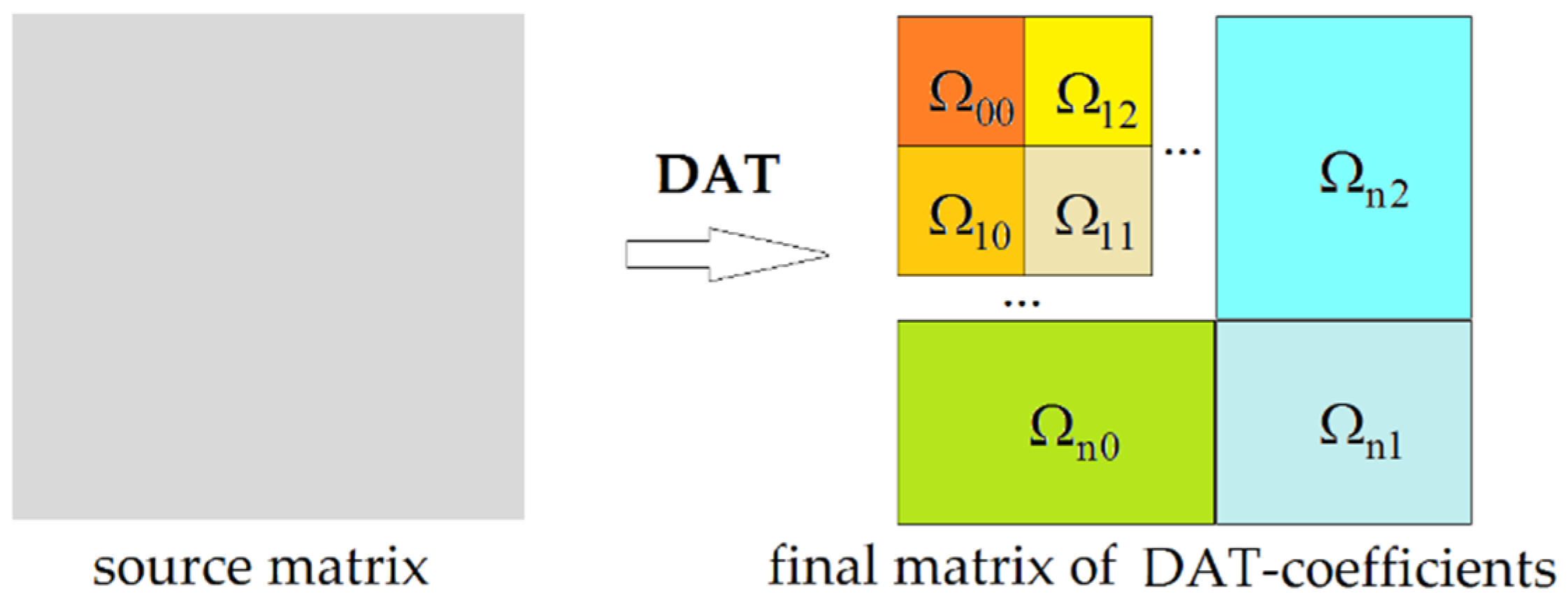
Consider another approach. First, array transform DAT of depth 1 is applied to each row of D and then to each column of the resulting matrix (Figure 4). In this way, a simple matrix transform, which is called DAT2, of depth 1 is built. The matrix of DAT-coefficients $\Omega$ is a result. This matrix has a block structure: the block ${\Omega }_{0,0}$ contains a small, aggregated copy of the source data D, all others contain DAT-coefficients of the corresponding orthogonal layers.

If we apply DAT2 of depth 1 to the block ${\Omega }_{00}$, i.e., left upper block, we obtain the matrix transform, which is called DAT2 of depth 2. In the same way, the matrix transform DAT2 of any valid depth n is constructed (Figure 5). Such a transform belongs to classic wavelet transforms that are widely used in image compression [58,60].

It is clear that DAT1 and DAT2 are significantly different. The output matrices have different structures, and their elements have different meanings. For this reason, complete information about the matrix transform applied is required in order to reconstruct the original matrix D.

Note that various mixtures of DAT1 and DAT2 can be applied. For example, first, DAT2 of the depth 1 can be applied, and then each block of the resulting matrix can be transformed by DAT1 (Figure 6). In addition, different combinations of DAT-procedure reuse can be applied to blocks of the matrix obtained at the previous step.

Hence, there is a great variety of constructions of the two-dimensional DAT. We stress that any attempt to correctly reconstruct the source matrix D using the given matrix of DAT-coefficients $\Omega$ requires huge computational resources if comprehensive information about DAT-procedure applied is absent. Moreover, the source matrix can be divided into blocks, each of which can be then transformed by DAT. Notice that this approach is used in such algorithms as JPEG [61] and WebP [62].

It is obvious that changes in the structure of DAT affect the DAC efficiency including complexity, memory savings, and metrics of quality loss. For this reason, the following question is of particular interest: what is the dependence of the DAC compression efficiency on the structure of DAT applied? An answer to this question makes it possible to choose such a structure of DAT that provides the best results with respect to different criteria.

In [47], DAT1 of the depth 5 and DAT2 of the depth 5 were considered, and it was shown that they provided almost the same compression ratio with the same distortions measured by RMSE (actually, only one compression mode of DAC, which provides the average RMSE = 2.8913, was considered), i.e., a significant variation of DAT structure does not reduce the efficiency of the DAC. It was proposed to apply this feature in order to provide protection of digital images.

Further, we compare DAT1 and DAT2. In opposite to [47], in the current research, a greater number of DAT structures is considered. Moreover, analysis is carried out for a wider range of quality loss levels. It will be shown that almost the same results can be obtained using these principally different matrix transforms. In other words, a significant variation of DAT structure does not significantly affect the processing results. For this reason, it is natural to expect that other intermediate structures of DAT provide practically the same compression results.

The following combination of features makes the algorithm DAC a promising tool for image protection and compression:

• a great variety of structures of the procedure DAT, which is a core of DAC;
• a possibility to reconstruct the source image correctly if and only if the correct inverse transform is applied;
• almost the same compression efficiency provided by different structures of DAT.

It is obvious that if DAC is used in some software, a key containing information about the structure of DAT applied should not be stored in the compressed file in order to provide protection of image content. If this requirement is satisfied, then a high level of privacy protection is guaranteed. If unauthorized persons obtain access to file and compression technology, but do not have the key, then correct content reconstruction requires great computational resources. Such a hack can be performed with more complication by encrypting some elements of the file with a compressed image.

Consider some special data structure requirements. Different variants of the matrix form DAT are based on one-dimensional DAT, i.e., DAT of an array. From functional properties of atomic wavelets [57], which constitute a core of DAT, it follows that a length of the source array A should be equal to $\mathrm{l}\mathrm{e}\mathrm{n}\mathrm{g}\mathrm{t}\mathrm{h}(\mathrm{A})=\mathrm{s}·2^{\mathrm{n}}$, where n is a depth of the DAT and s is some integer. This restriction is called the length condition. If it is not satisfied, then it is suggested to extend A such that equality holds. We propose to fill extra elements by values, which are equal to the last element of A. In this case, the extended version of A has up to $2^{\mathrm{n}}-1$ extra elements. When processing the matrix M, its rows and columns should also satisfy the length condition, defined by the structure of DAT. In order to provide such satisfaction, it is proposed to add extra columns, each of which coincides with the last column of M, and after that to add extra rows using the same approach. This provides a possibility to apply the DAT of any structure to a matrix of any size.

2.3. Quality Loss Control Mechanism

DAC is the lossy compression algorithm. Main distortions occur during the quantization of DAT-coefficients. It is clear that appropriate coefficients of quantization should be used. In the standards of some algorithms (for instance, JPEG), the recommended values are given. However, sometimes developers of software and devices apply their own coefficients. We stress that loss of quality depends a lot on quantization coefficients. For this reason, their choice should provide fulfillment of requirements for the quality in terms of some given metrics.

In [60], a quality loss control mechanism for the algorithm DAC was introduced. It provides the possibility to obtain the desired distortions measured by maximum absolute deviation (MAD) often used in remote sensing [22,23]. Basically, this metric is defined by the formula

$$\mathrm{M}\mathrm{A}\mathrm{D}=\underset{\mathrm{i},\mathrm{j}}{\max }\left|{\mathrm{X}}_{\mathrm{i}\mathrm{j}}-{\mathrm{Y}}_{\mathrm{i}\mathrm{j}}\right|,$$

where $\mathrm{X}=\left({\mathrm{X}}_{\mathrm{i}\mathrm{j}}\right),\mathrm{Y}=\left({\mathrm{Y}}_{\mathrm{i}\mathrm{j}}\right)$ are the source and reconstructed images, respectively. For the case of full-color digital images, the MAD-metric is built as follows:

$$\mathrm{M}\mathrm{A}\mathrm{D}=\underset{\mathrm{i},\mathrm{j}}{\max }\left\{\left|{\mathrm{X}}_{\mathrm{i}\mathrm{j}}^{[\mathrm{R}]}-{\mathrm{Y}}_{\mathrm{i}\mathrm{j}}^{[\mathrm{R}]}\right|,\left|{\mathrm{X}}_{\mathrm{i}\mathrm{j}}^{[\mathrm{G}]}-{\mathrm{Y}}_{\mathrm{i}\mathrm{j}}^{[\mathrm{G}]}\right|,\left|{\mathrm{X}}_{\mathrm{i}\mathrm{j}}^{[\mathrm{B}]}-{\mathrm{Y}}_{\mathrm{i}\mathrm{j}}^{[\mathrm{B}]}\right|\right\},$$

where $\left({\mathrm{X}}_{\mathrm{i}\mathrm{j}}^{[\mathrm{R}]},{\mathrm{X}}_{\mathrm{i}\mathrm{j}}^{[\mathrm{G}]},{\mathrm{X}}_{\mathrm{i}\mathrm{j}}^{[\mathrm{B}]}\right), \left({\mathrm{Y}}_{\mathrm{i}\mathrm{j}}^{[\mathrm{R}]},{\mathrm{Y}}_{\mathrm{i}\mathrm{j}}^{[\mathrm{G}]},{\mathrm{Y}}_{\mathrm{i}\mathrm{j}}^{[\mathrm{B}]}\right)$ are RGB-components of pixels ${\mathrm{X}}_{\mathrm{i}\mathrm{j}}$ and ${\mathrm{Y}}_{\mathrm{i}\mathrm{j}}$.

High sensitivity even to minor distortions is a key feature of MAD. Note that if MAD is small, then quality loss, which is obtained during processing (e.g., due to lossy compression), is insignificant. If MAD is large, then it means that at least one pixel is changed considerably. Although, if only several pixels have significant changes of color intensity, visual quality might remain high, especially when processing high-resolution images. Hence, MAD-metric should be used as a metric of distortions in the case of low-quality loss or near lossless compression.

Consider the quality loss control mechanism, which was proposed in [60], in more detail. It is based on an estimate concerning the expansion (1).

We start with the transform DAT1 and the case of grayscale image processing. Let D be a source matrix. Using DAT1, we obtain the matrix $\Omega$ that consists of blocks ${\left\{{\Omega }_{\mathrm{i},\mathrm{j}}\right\}}_{\mathrm{i},\mathrm{j}=0}^{\mathrm{n}}$ (see Figure 3). Denote by ${\left\{{\mathsf{\delta }}_{\mathrm{i},\mathrm{j}}\right\}}_{\mathrm{i},\mathrm{j}=0}^{\mathrm{n}}$ a set of positive real numbers. Consider the following quantization procedure:

$${\Psi }_{0,0}=\mathrm{R}\mathrm{o}\mathrm{u}\mathrm{n}\mathrm{d}\left(\frac{{\Omega }_{0,0}}{{\mathsf{\delta }}_{0,0}}\right), {\Psi }_{0,\mathrm{j}}=\mathrm{R}\mathrm{o}\mathrm{u}\mathrm{n}\mathrm{d}\left(\frac{2^{2\mathrm{j}-1}{\Omega }_{0,\mathrm{j}}}{{\mathsf{\delta }}_{0,\mathrm{j}}}\right) \mathrm{for} \mathrm{j}=1,\dots ,\mathrm{n},$$

(2)

$${\Psi }_{\mathrm{i},0}=\mathrm{R}\mathrm{o}\mathrm{u}\mathrm{n}\mathrm{d}\left(\frac{2^{2\mathrm{i}-1}{\Omega }_{\mathrm{i},0}}{{\mathsf{\delta }}_{\mathrm{i},0}}\right) \mathrm{for} \mathrm{i}=1,\dots ,\mathrm{n} \mathrm{and} {\Psi }_{\mathrm{i},\mathrm{j}}=\mathrm{R}\mathrm{o}\mathrm{u}\mathrm{n}\mathrm{d}\left(\frac{2^{2(\mathrm{i}+\mathrm{j}-1)}{\Omega }_{\mathrm{i},\mathrm{j}}}{{\mathsf{\delta }}_{\mathrm{i},\mathrm{j}}}\right) \mathrm{for} \mathrm{i}, \mathrm{j}=1,\dots ,\mathrm{n}.$$

(3)

It is presented in matrix form. We assume that all operations are applied to each element of blocks. Using (2), (3), the matrix $\Psi ={\left({\Psi }_{\mathrm{i},\mathrm{j}}\right)}_{\mathrm{i},\mathrm{j}=0}^{\mathrm{n}}$ is computed. In DAC, blocks of this matrix are encoded using binary AC.

Dequantization is constructed as follows:

$${\tilde{\Omega }}_{0,0}={\mathsf{\delta }}_{0,0}{\Psi }_{0,0}, {\tilde{\Omega }}_{0,\mathrm{j}}=\frac{{\mathsf{\delta }}_{0,\mathrm{j}}}{2^{2\mathrm{j}-1}}{\Psi }_{0,\mathrm{j}} \mathrm{for} \mathrm{j}=1,\dots , \mathrm{n},$$

(4)

$${\tilde{\Omega }}_{\mathrm{i},0}=\frac{{\mathsf{\delta }}_{\mathrm{i},0}}{2^{2\mathrm{i}-1}}{\Psi }_{\mathrm{i},0} \mathrm{for} \mathrm{i}=1,\dots , \mathrm{n} \mathrm{and} {\tilde{\Omega }}_{\mathrm{i},\mathrm{j}}=\frac{{\mathsf{\delta }}_{\mathrm{i},\mathrm{j}}}{2^{2(\mathrm{i}+\mathrm{j}-1)}}{\Psi }_{\mathrm{i},\mathrm{j}} \mathrm{for} \mathrm{i}, \mathrm{j}=1,\dots , \mathrm{n}.$$

(5)

This procedure provides computation of the matrix $\tilde{\Omega }={\left\{{\tilde{\Omega }}_{\mathrm{i},\mathrm{j}}\right\}}_{\mathrm{i},\mathrm{j}=0}^{\mathrm{n}}$ that is further used in order to obtain $\tilde{\mathrm{D}}$, which is a matrix of the decompressed image.

It follows that if (2)–(5) are applied, then

$$\mathrm{M}\mathrm{A}\mathrm{D}\le {\displaystyle \sum _{\mathrm{i},\mathrm{j}=0}^{\mathrm{n}}{\mathsf{\delta }}_{\mathrm{i},\mathrm{j}}}.$$

(6)

The right part of this inequality is an upper bound of MAD. We denote it by UBMAD. In other words, the proposed quantization and dequantization procedures provides that loss of quality measured by MAD is not greater than UBMAD, which is defined by parameters of quantization ${\left\{{\mathsf{\delta }}_{\mathrm{i},\mathrm{j}}\right\}}_{\mathrm{i},\mathrm{j}=0}^{\mathrm{n}}$. As it can be seen, DAT-coefficients corresponding to the same wavelet layer are quantized using the same quantization coefficient.

When processing full-color digital image, we propose to apply the same approach. Consider three sets of positive real numbers ${\left\{{\mathsf{\delta }}_{\mathrm{i},\mathrm{j}}^{[\mathrm{Y}]}\right\}}_{\mathrm{i},\mathrm{j}=0}^{\mathrm{n}}$, ${\left\{{\mathsf{\delta }}_{\mathrm{i},\mathrm{j}}^{[\mathrm{C}\mathrm{r}]}\right\}}_{\mathrm{i},\mathrm{j}=0}^{\mathrm{n}}$ and ${\left\{{\mathsf{\delta }}_{\mathrm{i},\mathrm{j}}^{[\mathrm{C}\mathrm{b}]}\right\}}_{\mathrm{i},\mathrm{j}=0}^{\mathrm{n}}$. Each of these sets is used in (2)–(5) for quantizing and dequantizing of matrices Ω^[Y], Ω^[Cr], Ω^[Cb] of DAT-coefficients corresponding to Y, Cr, and Cb respectively. In this case,

$$\mathrm{M}\mathrm{A}\mathrm{D}\le \max \left\{{\displaystyle \sum _{\mathrm{i},\mathrm{j}=0}^{\mathrm{n}}{\mathsf{\delta }}_{\mathrm{i},\mathrm{j}}^{[\mathrm{Y}]}},{\displaystyle \sum _{\mathrm{i},\mathrm{j}=0}^{\mathrm{n}}{\mathsf{\delta }}_{\mathrm{i},\mathrm{j}}^{[\mathrm{C}\mathrm{r}]}},{\displaystyle \sum _{\mathrm{i},\mathrm{j}=0}^{\mathrm{n}}{\mathsf{\delta }}_{\mathrm{i},\mathrm{j}}^{[\mathrm{C}\mathrm{b}]}}\right\}.$$

(7)

where the right part is a maximum of three values, each of which is a sum of real numbers introduced above. This maximum is denoted by UBMAD.

Further, consider the transform DAT2, which is used for grayscale image compressing. A result of the application of DAT2 to the matrix D of the image processed is the matrix Ω that consists of blocks ${\left\{{\Omega }_{0,0},{\Omega }_{\mathrm{k},0},{\Omega }_{\mathrm{k},1},{\Omega }_{\mathrm{k},2}\right\}}_{\mathrm{k}=1}^{\mathrm{n}}$ (see Figure 5). Let ${\left\{{\mathsf{\delta }}_{0,0},{\mathsf{\delta }}_{\mathrm{k},0},{\mathsf{\delta }}_{\mathrm{k},1},{\mathsf{\delta }}_{\mathrm{k},2}\right\}}_{\mathrm{k}=1}^{\mathrm{n}}$ be a set of positive numbers. As before, these values are used in quantizing blocks of the matrix Ω. This procedure is:

$${\Psi }_{0,0}=\mathrm{R}\mathrm{o}\mathrm{u}\mathrm{n}\mathrm{d}\left(\frac{{\Omega }_{0,0}}{{\mathsf{\delta }}_{0,0}}\right), {\Psi }_{\mathrm{k},0}=\mathrm{R}\mathrm{o}\mathrm{u}\mathrm{n}\mathrm{d}\left(\frac{2^{2\mathrm{k}-1}{\Omega }_{\mathrm{k},0}}{{\mathsf{\delta }}_{\mathrm{k},0}}\right),$$

(8)

$${\Psi }_{\mathrm{k},1}=\mathrm{R}\mathrm{o}\mathrm{u}\mathrm{n}\mathrm{d}\left(\frac{2^{2(2\mathrm{k}-1)}{\Omega }_{\mathrm{k},1}}{{\mathsf{\delta }}_{\mathrm{k},1}}\right) \mathrm{and} {\Psi }_{\mathrm{k},2}=\mathrm{R}\mathrm{o}\mathrm{u}\mathrm{n}\mathrm{d}\left(\frac{2^{2\mathrm{k}-1}{\Omega }_{\mathrm{k},2}}{{\mathsf{\delta }}_{\mathrm{k},2}}\right) \mathrm{for} \mathrm{k}=1,\dots , \mathrm{n}.$$

(9)

Dequantization is built as follows:

$${\tilde{\Omega }}_{0,0}={\mathsf{\delta }}_{0,0}{\Psi }_{0,0}, {\tilde{\Omega }}_{\mathrm{k},0}=\frac{{\mathsf{\delta }}_{\mathrm{k},0}}{2^{2\mathrm{k}-1}}{\Psi }_{\mathrm{k},0},$$

(10)

$${\tilde{\Omega }}_{\mathrm{k},1}=\frac{{\mathsf{\delta }}_{\mathrm{k},1}}{2^{2(2\mathrm{k}-1)}}{\Psi }_{\mathrm{k},1} \mathrm{and} {\tilde{\Omega }}_{\mathrm{k},2}=\frac{{\mathsf{\delta }}_{\mathrm{k},2}}{2^{2\mathrm{k}-1}}{\Psi }_{\mathrm{k},2} \mathrm{for} \mathrm{k}=1,\dots , \mathrm{n}.$$

(11)

Computation of the matrix $\tilde{\Omega }$, which is used in order to obtain the decompressed image, is provided by (10), (11). Quality loss measured by MAD satisfies the following inequality:

$$\mathrm{M}\mathrm{A}\mathrm{D}\le {\mathsf{\delta }}_{0,0}+{\displaystyle \sum _{\mathrm{k}=1}^{\mathrm{n}}\left({\mathsf{\delta }}_{\mathrm{k},0}+{\mathsf{\delta }}_{\mathrm{k},1}+{\mathsf{\delta }}_{\mathrm{k},2}\right)}.$$

(12)

By UBMAD, we denote the right part of this expression.

In the case of full-color image compression using DAC with DAT2, the same can be used. Three sets ${\left\{{\mathsf{\delta }}_{0,0}^{[\mathrm{Y}]},{\mathsf{\delta }}_{\mathrm{k},0}^{[\mathrm{Y}]},{\mathsf{\delta }}_{\mathrm{k},1}^{[\mathrm{Y}]},{\mathsf{\delta }}_{\mathrm{k},2}^{[\mathrm{Y}]}\right\}}_{\mathrm{k}=1}^{\mathrm{n}}$, ${\left\{{\mathsf{\delta }}_{0,0}^{[\mathrm{C}\mathrm{r}]},{\mathsf{\delta }}_{\mathrm{k},0}^{[\mathrm{C}\mathrm{r}]},{\mathsf{\delta }}_{\mathrm{k},1}^{[\mathrm{C}\mathrm{r}]},{\mathsf{\delta }}_{\mathrm{k},2}^{[\mathrm{C}\mathrm{r}]}\right\}}_{\mathrm{k}=1}^{\mathrm{n}}$ and ${\left\{{\mathsf{\delta }}_{0,0}^{[\mathrm{C}\mathrm{b}]},{\mathsf{\delta }}_{\mathrm{k},0}^{[\mathrm{C}\mathrm{b}]},{\mathsf{\delta }}_{\mathrm{k},1}^{[\mathrm{C}\mathrm{b}]},{\mathsf{\delta }}_{\mathrm{k},2}^{[\mathrm{C}\mathrm{b}]}\right\}}_{\mathrm{k}=1}^{\mathrm{n}}$ are applied as parameters of quantization. In order to obtain formulas for quantizing and dequantizing the matrices Ω^[Y], Ω^[Cr], Ω^[Cb], one should put these values to (8)–(11). In this case, the following inequality holds:

$$\begin{gathered} \mathrm{M}\mathrm{A}\mathrm{D}\le \max \{{\mathsf{\delta }}_{0,0}^{[\mathrm{Y}]}+{\displaystyle \sum _{\mathrm{k}=1}^{\mathrm{n}}\left({\mathsf{\delta }}_{\mathrm{k},0}^{[\mathrm{Y}]}+{\mathsf{\delta }}_{\mathrm{k},1}^{[\mathrm{Y}]}+{\mathsf{\delta }}_{\mathrm{k},2}^{[\mathrm{Y}]}\right)}, {\mathsf{\delta }}_{0,0}^{[\mathrm{C}\mathrm{r}]}+{\displaystyle \sum _{\mathrm{k}=1}^{\mathrm{n}}\left({\mathsf{\delta }}_{\mathrm{k},0}^{[\mathrm{C}\mathrm{r}]}+{\mathsf{\delta }}_{\mathrm{k},1}^{[\mathrm{C}\mathrm{r}]}+{\mathsf{\delta }}_{\mathrm{k},2}^{[\mathrm{C}\mathrm{r}]}\right)}, \\ {\mathsf{\delta }}_{0,0}^{[\mathrm{C}\mathrm{b}]}+{\displaystyle \sum _{\mathrm{k}=1}^{\mathrm{n}}\left({\mathsf{\delta }}_{\mathrm{k},0}^{[\mathrm{C}\mathrm{b}]}+{\mathsf{\delta }}_{\mathrm{k},1}^{[\mathrm{C}\mathrm{b}]}+{\mathsf{\delta }}_{\mathrm{k},2}^{[\mathrm{C}\mathrm{b}]}\right)}\}. \end{gathered}$$

(13)

Further, the right part of (13) is denoted by UBMAD.

This implies that (2)–(5) in combination with (6), (7) and (8)–(11) in combination with (12), (13) provide control of quality loss measured by MAD-metric when compressing digital images by DAC with DAT1 and DAT2, respectively.

It is obvious that (6), (7), (12), and (13) are upper bounds. Application of the proposed methods of quantization and dequantization does not provide obtaining MAD, which is equal to the desired value. Nevertheless, the following property is guaranteed: quality loss measured by this metric does not exceed the given value. This feature is important if a minor loss of quality is required.

The choice of parameters $\left\{{\mathsf{\delta }}_{\mathrm{i},\mathrm{j}}\right\}$ or $\left\{{\mathsf{\delta }}_{\mathrm{i},\mathrm{j}}^{[\mathrm{Y}]},{\mathsf{\delta }}_{\mathrm{i},\mathrm{j}}^{[\mathrm{C}\mathrm{r}]},{\mathsf{\delta }}_{\mathrm{i},\mathrm{j}}^{[\mathrm{C}\mathrm{b}]}\right\}$, when processing respectively grayscale or full-color images, defines quality loss settings of DAC. Many lossy compression algorithms, including DAC, have the following feature: if one fixes some setting of quality and processes two images of different content complexity, results of non-equal distortions are usually obtained. Hence, the following question is of particular interest: what is a variation of compression efficiency indicators? In the next section, we study this question. Besides, as has been mentioned above, the metric MAD might be a non-adequate measure of distortions if its value is large. In this case, other quality loss indicators, in particular, RMSE and PSNR can be used:

$$\begin{gathered} \mathrm{R}\mathrm{M}\mathrm{S}\mathrm{E}=\sqrt{\frac{1}{3\mathrm{m}\mathrm{n}}{\displaystyle \sum _{\mathrm{i},\mathrm{j}=1}^{\mathrm{m},\mathrm{n}}\left({\left({\mathrm{X}}_{\mathrm{i}\mathrm{j}}^{[\mathrm{R}]}-{\mathrm{Y}}_{\mathrm{i}\mathrm{j}}^{[\mathrm{R}]}\right)}^2+{\left({\mathrm{X}}_{\mathrm{i}\mathrm{j}}^{[\mathrm{G}]}-{\mathrm{Y}}_{\mathrm{i}\mathrm{j}}^{[\mathrm{B}]}\right)}^2+{\left({\mathrm{X}}_{\mathrm{i}\mathrm{j}}^{[\mathrm{B}]}-{\mathrm{Y}}_{\mathrm{i}\mathrm{j}}^{[\mathrm{b}]}\right)}^2\right)}}, \\ \mathrm{P}\mathrm{S}\mathrm{N}\mathrm{R}=20{\log }_{10}\frac{255}{\mathrm{R}\mathrm{M}\mathrm{S}\mathrm{E}}, \end{gathered}$$

where ${\mathrm{X}}_{\mathrm{i}\mathrm{j}}=\left({\mathrm{X}}_{\mathrm{i}\mathrm{j}}^{[\mathrm{R}]},{\mathrm{X}}_{\mathrm{i}\mathrm{j}}^{[\mathrm{G}]},{\mathrm{X}}_{\mathrm{i}\mathrm{j}}^{[\mathrm{B}]}\right), {\mathrm{Y}}_{\mathrm{i}\mathrm{j}}=\left({\mathrm{Y}}_{\mathrm{i}\mathrm{j}}^{[\mathrm{R}]},{\mathrm{Y}}_{\mathrm{i}\mathrm{j}}^{[\mathrm{G}]},{\mathrm{Y}}_{\mathrm{i}\mathrm{j}}^{[\mathrm{B}]}\right)$ are pixels of RGB-images X and Y, which are respectively the source and the reconstructed images of the size $\mathrm{m}\times \mathrm{n}$.

Further, we investigate the correlation of these metrics and MAD, as well as their dependence on UBMAD. For this purpose, a set of 100 test images is used. Each of them is processed using the algorithm DAC with different quality loss settings and structures of DAT.

3. Discrete Atomic Compression of Test Data

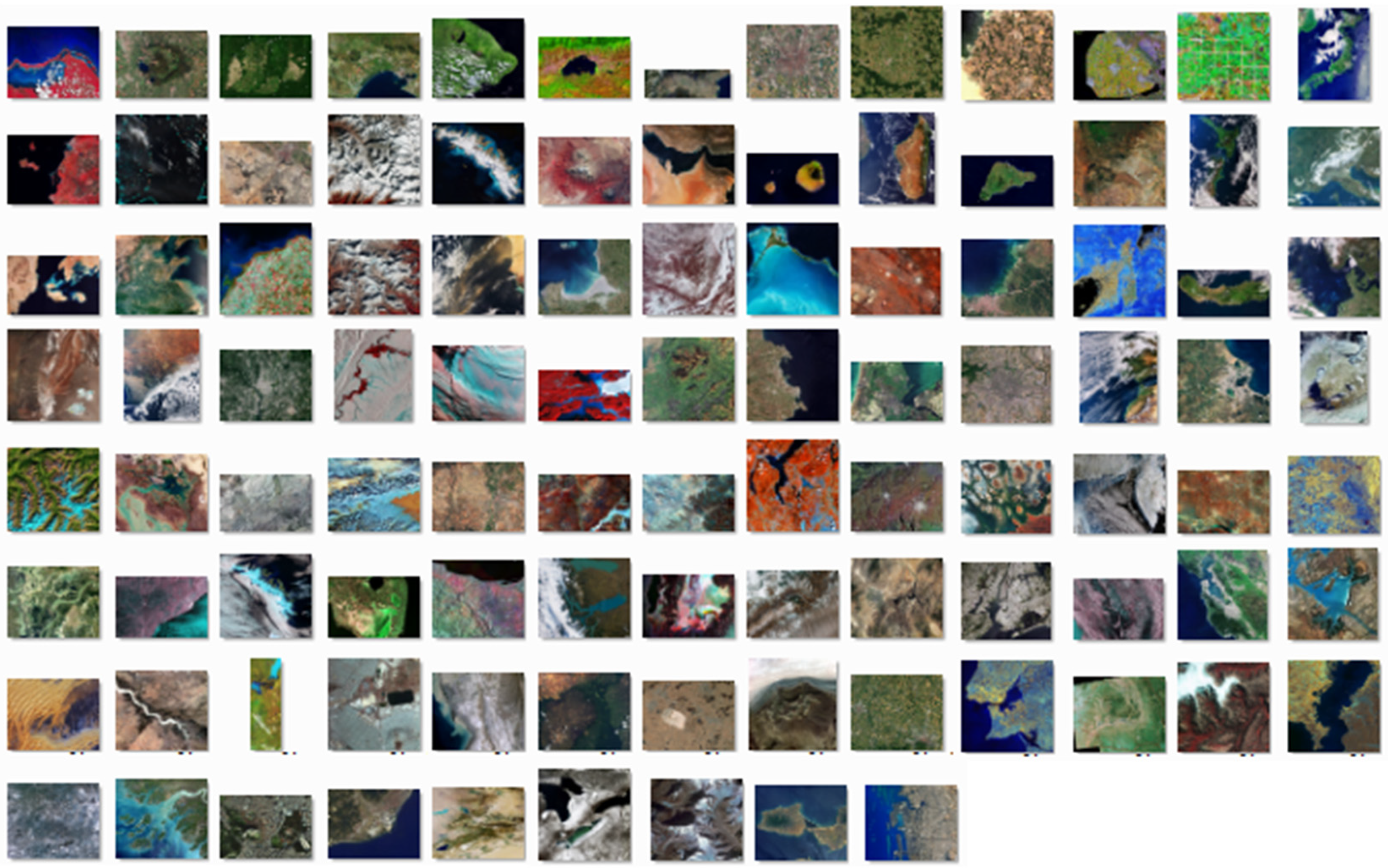
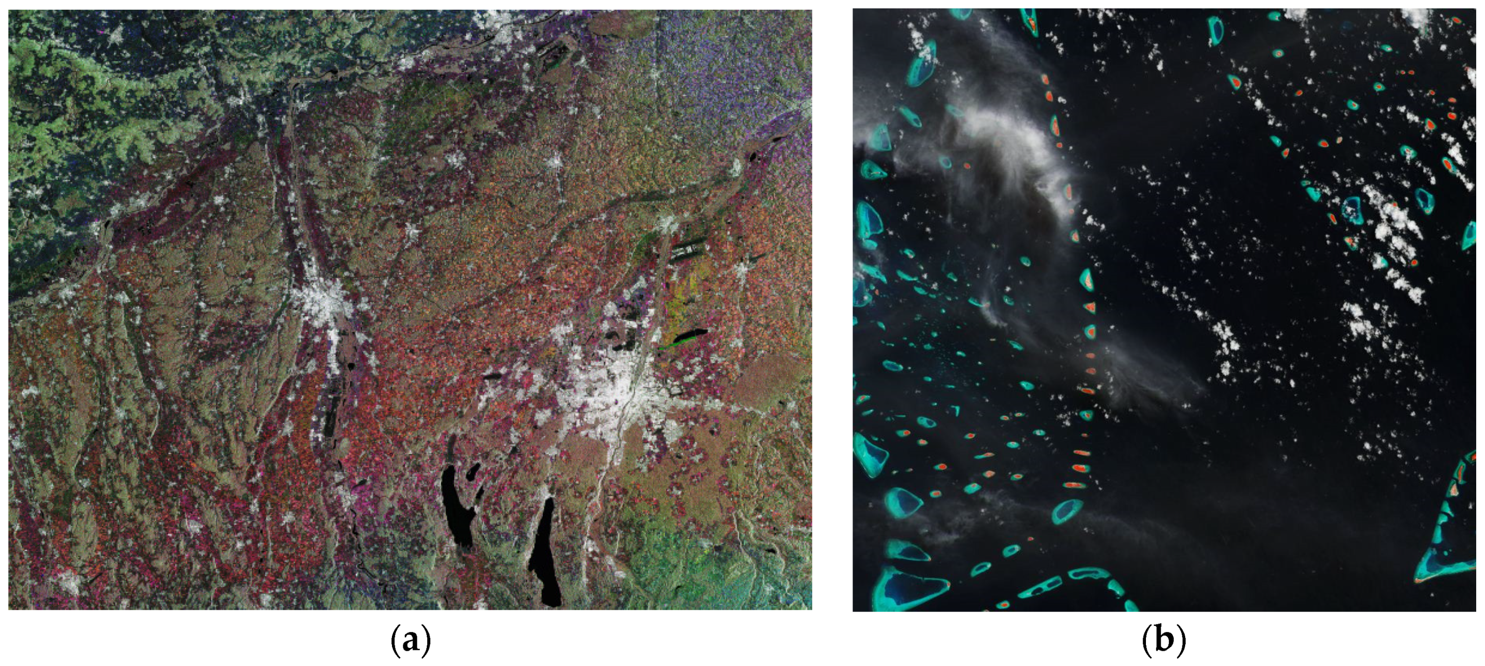
In the current research, we used 100 digital images (see Figure 7) of the European Space Agency (ESA). They were downloaded from ESA official site: https://www.esa.int/ESA_Multimedia/Images, accessed on 27 October 2021. In addition, these test data are available at the link to Google-drive folder (here, RGB-images in BMP-format, short information about them, and tables with results of their processing can be found): https://drive.google.com/drive/folders/1PSld3GqFQJYfrNs_b4uaxieY4m3AlwW2?usp=sharing, accessed on 27 October 2021. One of the principal features of the test data applied is the presence of a great number of small details and sharp changes of color (Figure 8a).

In other words, mostly images with complex content are used. However, some of them contain domains of relatively constant color in combination with smooth color changes (Figure 8b).

For testing purposes, it can be used in situ datasets too. These data can be collected during different land surveys, for example along the roads (Figure 9), and can be especially useful for crop classification. During data preprocessing, it could be prepared small polygons, which can be some representation of different homogeneous land cover classes.

Each of the test images is processed by the algorithms DAC with DAT1 of the depth 5 and DAT2 with the depth n = 1, 2, 3, 4, and 5. Different quality loss settings, which are defined by the values $\left\{{\mathsf{\delta }}_{\mathrm{i},\mathrm{j}}^{[\mathrm{Y}]},{\mathsf{\delta }}_{\mathrm{i},\mathrm{j}}^{[\mathrm{C}\mathrm{r}]},{\mathsf{\delta }}_{\mathrm{i},\mathrm{j}}^{[\mathrm{C}\mathrm{b}]}\right\}$, are used. The following steps are applied:

(1)

fix the structure of DAT and its depth in the case of DAT2;

(2)

fix parameters $\left\{{\mathsf{\delta }}_{\mathrm{i},\mathrm{j}}^{[\mathrm{Y}]},{\mathsf{\delta }}_{\mathrm{i},\mathrm{j}}^{[\mathrm{C}\mathrm{r}]},{\mathsf{\delta }}_{\mathrm{i},\mathrm{j}}^{[\mathrm{C}\mathrm{b}]}\right\}$ and compute UBMAD;

(3)

for each test image perform the following:

–

compress the current image;

–

compute compression ratio (CR): $\mathrm{CR}=\frac{\mathrm{size} \mathrm{of} \mathrm{source} \mathrm{file}}{\mathrm{size} \mathrm{of} \mathrm{cimpressed} \mathrm{file}}$;

–

decompress image;

–

compute quality loss measured by MAD, RMSE, and PSNR;

–

store results in Table.

In this paper, Tables with the results obtained are not given due to their huge size (these data are presented in files Efficiency_indicators.pdf, ESA_data_DAT_1.xlsx, and ESA_data_DAT_2.xlsx, which are available at the link to Google-drive folder https://drive.google.com/drive/folders/1PSld3GqFQJYfrNs_b4uaxieY4m3AlwW2?usp=sharing, accessed on 27 October 2021). Further, we present their analysis.

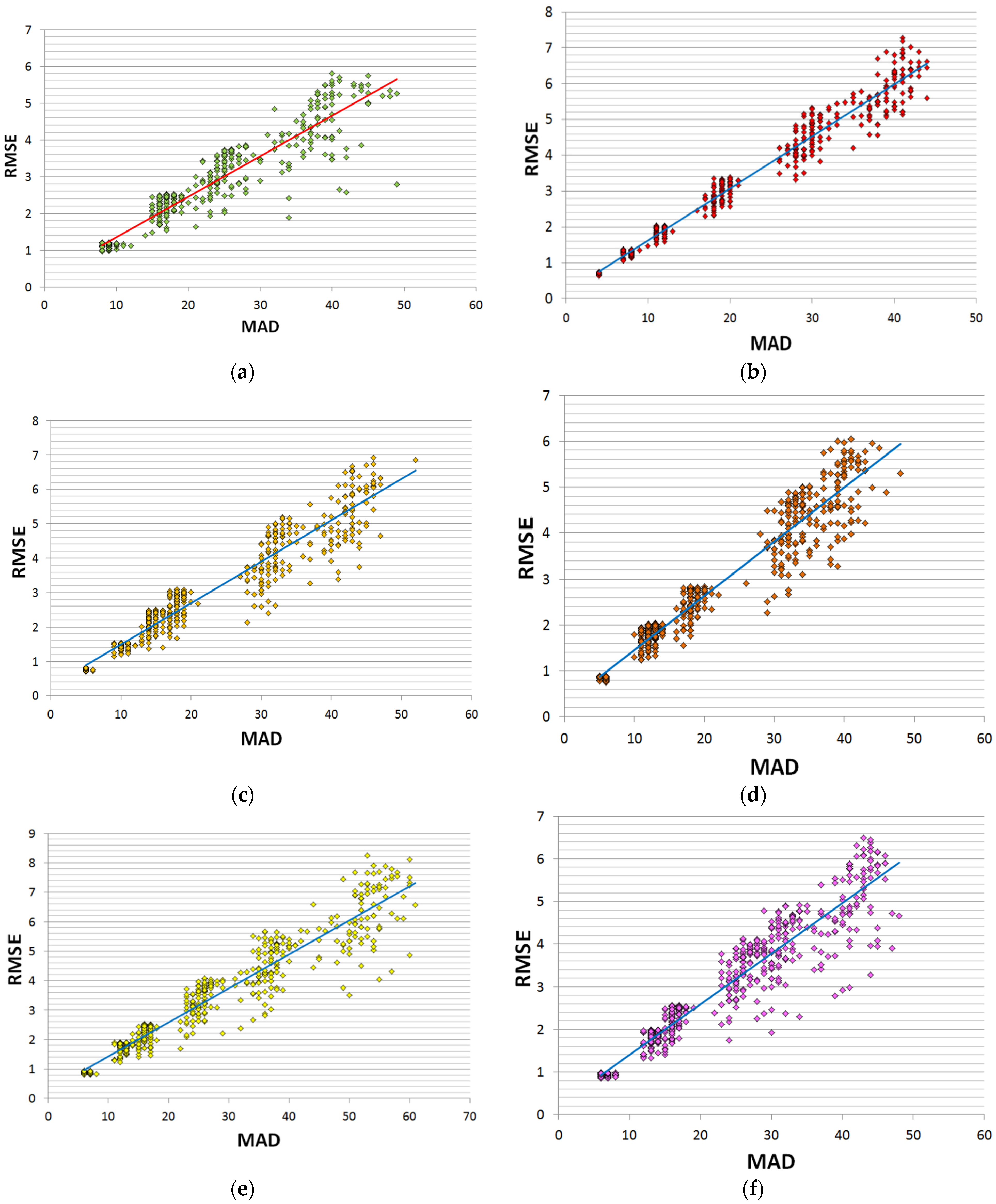
First, we study the correlation of quality loss metrics RMSE, PSNR, and MAD. Since PSNR is a function of RMSE, it is sufficient to investigate the dependence of RMSE on MAD. In Figure 10, scatter plots of RMSE vs. MAD are shown. In addition, we have computed Pearson’s correlation coefficient R and Spearman’s rank-order correlation coefficient $\mathsf{\rho }$ [63]. Moreover, using the least-square method [63], linear regression equations have been constructed. Their graphs are also given in Figure 10. In

Table 1. Indicators of correlation of MAD and RMSE for different structures of DAT.

Structure of DAT	Pearson’s Correlation Coefficient	Spearman’s Rank Correlation Coefficients	Parameters of Linear Regression		$\mathbf{Value} \mathbf{of} \mathbf{Test} \mathbf{Statistic} \overline{\mathbf{F}}$
			a	b
DAT1 of the depth 5	0.936	0.940	0.110	0.264	2802.34
DAT2 of the depth 1	0.988	0.985	0.145	0.173	23,608.65
DAT2 of the depth 2	0.963	0.967	0.120	0.285	7624.15
DAT2 of the depth 3	0.965	0.954	0.118	0.272	8181.95
DAT2 of the depth 4	0.960	0.967	0.116	0.270	7172.21
DAT2 of the depth 5	0.948	0.952	0.118	0.222	5292.41

, values of R, $\mathsf{\rho }$, as well as coefficients a, b of the linear equation $\mathrm{y}=\mathrm{a}\mathrm{x}+\mathrm{b}$, where y = RMSE and x = MAD, are presented.

Furthermore, using the ANOVA F-test [64], we have checked whether there is a linear regression relationship between RMSE and MAD. For this purpose, the following test statistic has been computed:

$$\overline{\mathrm{F}}=\frac{{\displaystyle \sum _{\mathrm{i}=1}^{\mathrm{n}}{\left({\widehat{\mathrm{y}}}_{\mathrm{i}}-\overline{\mathrm{y}}\right)}^2}}{\frac{1}{\mathrm{n}-2}{\displaystyle \sum _{\mathrm{i}=1}^{\mathrm{n}}{\left({\mathrm{y}}_{\mathrm{i}}-{\widehat{\mathrm{y}}}_{\mathrm{i}}\right)}^2}},$$

where n = 100 is the number of analyzed values, $\left\{{\mathrm{y}}_1,\dots ,{\mathrm{y}}_{\mathrm{n}}\right\}$ is a set of RMSE-values and $\overline{\mathrm{y}}=\frac{1}{\mathrm{n}}{\displaystyle \sum _{\mathrm{i}=1}^{\mathrm{n}}{\mathrm{y}}_{\mathrm{i}}}$; ${\widehat{\mathrm{y}}}_{\mathrm{i}}=\mathrm{a}{\mathrm{x}}_{\mathrm{i}}+\mathrm{b}$, where a, b are coefficients of linear regression, $\left\{{\mathrm{x}}_1,\dots ,{\mathrm{x}}_{\mathrm{n}}\right\}$ are values of MAD. Here, we note that the point $\left({\mathrm{x}}_{\mathrm{i}},{\mathrm{y}}_{\mathrm{i}}\right)$ is a pair of quality loss values measured by MAD and RMSE for an i-th test image. In Table 1, values of $\overline{\mathrm{F}}$ are given. This statistic is compared with ${\mathrm{F}}_{1,\mathrm{n}-2}$ from F-table [64]. Currently, ${\mathrm{F}}_{1,\mathrm{n}-2}=3.865$. If $\overline{\mathrm{F}}>{\mathrm{F}}_{1,\mathrm{n}-2}$, then there is a linear regression between y and x, i.e., RMSE and MAD. It follows from Table 1 that, for each structure of DAT, there is the linear regression between quality loss indicators MAD and RMSE. This is also evidenced by the fact that values of both Pearson’s correlation and Spearman’s rank correlation coefficients are close to 1.

Second, we investigate a dependence of MAD, RMSE, PSNR and CR on UBMAD. For this purpose, we compute mean (E), minimum, maximum values and deviation ($\mathsf{\sigma }$) of these compression efficiency indicators for each value of UBMAD applied. In addition, we calculate percentage of values obtained that belongs to segments $\left[\mathrm{E}-\mathrm{k}\mathsf{\sigma },\mathrm{E}+\mathrm{k}\mathsf{\sigma }\right]$ for k = 1, 2 and 3. In other words, we estimate the scatter of experimental data with respect to the mean. In

Table 2. DAT1 of the depth 5: indicators of compression efficiency.

Indicator		UBMAD
		36	63	95	155
MAD	min	8	14	20	30
	max	12	20	30	49
	mean (E)	9.030	16.890	24.840	38.710
	deviation (σ)	0.688	1.154	2.135	4.103
	$\mathrm{percentage} \mathrm{of} \mathrm{values} \mathrm{in} \left[\mathrm{E}-\mathsf{\sigma },\mathrm{E}+\mathsf{\sigma }\right]$	67	81	66	65
	$\mathrm{percentage} \mathrm{of} \mathrm{values} \mathrm{in} \left[\mathrm{E}-2\mathsf{\sigma },\mathrm{E}+2\mathsf{\sigma }\right]$	97	98	96	94
	$\mathrm{percentage} \mathrm{of} \mathrm{values} \mathrm{in} \left[\mathrm{E}-3\mathsf{\sigma },\mathrm{E}+3\mathsf{\sigma }\right]$	99	100	100	100
RMSE	min	0.972	1.405	1.644	1.887
	max	1.210	2.524	3.849	5.806
	mean (E)	1.138	2.204	3.098	4.451
	deviation (σ)	0.056	0.272	0.500	0.856
	$\mathrm{percentage} \mathrm{of} \mathrm{values} \mathrm{in} \left[\mathrm{E}-\mathsf{\sigma },\mathrm{E}+\mathsf{\sigma }\right]$	77	69	68	68
	$\mathrm{percentage} \mathrm{of} \mathrm{values} \mathrm{in} \left[\mathrm{E}-2\mathsf{\sigma },\mathrm{E}+2\mathsf{\sigma }\right]$	93	96	95	96
	$\mathrm{percentage} \mathrm{of} \mathrm{values} \mathrm{in} \left[\mathrm{E}-3\mathsf{\sigma },\mathrm{E}+3\mathsf{\sigma }\right]$	100	100	100	100
PSNR, dB	min	46.473	40.090	36.424	32.854
	max	48.378	45.180	43.815	42.615
	mean (E)	47.017	41.340	38.433	35.343
	deviation (σ)	0.444	1.155	1.517	1.856
	$\mathrm{percentage} \mathrm{of} \mathrm{values} \mathrm{in} \left[\mathrm{E}-\mathsf{\sigma },\mathrm{E}+\mathsf{\sigma }\right]$	78	78	70	73
	$\mathrm{percentage} \mathrm{of} \mathrm{values} \mathrm{in} \left[\mathrm{E}-2\mathsf{\sigma },\mathrm{E}+2\mathsf{\sigma }\right]$	93	96	94	95
	$\mathrm{percentage} \mathrm{of} \mathrm{values} \mathrm{in} \left[\mathrm{E}-3\mathsf{\sigma },\mathrm{E}+3\mathsf{\sigma }\right]$	99	99	99	99
CR	min	1.236	1.595	1.817	2.146
	max	4.734	14.326	24.138	44.525
	mean (E)	2.269	3.769	4.940	7.376
	deviation (σ)	0.633	1.740	2.833	5.297
	$\mathrm{percentage} \mathrm{of} \mathrm{values} \mathrm{in} \left[\mathrm{E}-\mathsf{\sigma },\mathrm{E}+\mathsf{\sigma }\right]$	75	85	90	92
	$\mathrm{percentage} \mathrm{of} \mathrm{values} \mathrm{in} \left[\mathrm{E}-2\mathsf{\sigma },\mathrm{E}+2\mathsf{\sigma }\right]$	95	95	96	97
	$\mathrm{percentage} \mathrm{of} \mathrm{values} \mathrm{in} \left[\mathrm{E}-3\mathsf{\sigma },\mathrm{E}+3\mathsf{\sigma }\right]$	98	99	98	98

and

Table 3. DAT2 of the depth 2: indicators of compression efficiency.

Indicator		UBMAD
		7	14	20	25	46	64
MAD	min	5	9	13	15	27	34
	max	6	12	17	21	36	52
	mean (E)	5.030	10.180	14.480	17.860	31.300	42.360
	deviation (σ)	0.171	0.575	0.771	1.005	1.851	2.952
	$\mathrm{percentage} \mathrm{of} \mathrm{values} \mathrm{in} \left[\mathrm{E}-\mathsf{\sigma },\mathrm{E}+\mathsf{\sigma }\right]$	97	70	85	67	74	68
	$\mathrm{percentage} \mathrm{of} \mathrm{values} \mathrm{in} \left[\mathrm{E}-2\mathsf{\sigma },\mathrm{E}+2\mathsf{\sigma }\right]$	97	91	99	96	97	97
	$\mathrm{percentage} \mathrm{of} \mathrm{values} \mathrm{in} \left[\mathrm{E}-3\mathsf{\sigma },\mathrm{E}+3\mathsf{\sigma }\right]$	97	98	99	99	100	99
RMSE	min	0.704	1.146	1.367	1.405	2.135	3.276
	max	0.817	1.543	2.503	3.093	5.194	6.915
	mean (E)	0.774	1.452	2.172	2.569	4.043	5.287
	deviation (σ)	0.031	0.091	0.278	0.396	0.724	0.873
	$\mathrm{percentage} \mathrm{of} \mathrm{values} \mathrm{in} \left[\mathrm{E}-\mathsf{\sigma },\mathrm{E}+\mathsf{\sigma }\right]$	63	85	69	68	67	66
	$\mathrm{percentage} \mathrm{of} \mathrm{values} \mathrm{in} \left[\mathrm{E}-2\mathsf{\sigma },\mathrm{E}+2\mathsf{\sigma }\right]$	96	93	96	96	97	98
	$\mathrm{percentage} \mathrm{of} \mathrm{values} \mathrm{in} \left[\mathrm{E}-3\mathsf{\sigma },\mathrm{E}+3\mathsf{\sigma }\right]$	100	99	100	100	100	100
PSNR, dB	min	49.884	44.360	40.158	38.322	33.819	31.334
	max	51.179	46.943	45.414	45.172	41.541	37.827
	mean (E)	50.356	44.909	41.471	40.046	36.146	33.788
	deviation (σ)	0.348	0.571	1.196	1.454	1.668	1.483
	$\mathrm{percentage} \mathrm{of} \mathrm{values} \mathrm{in} \left[\mathrm{E}-\mathsf{\sigma },\mathrm{E}+\mathsf{\sigma }\right]$	64	87	77	72	70	68
	$\mathrm{percentage} \mathrm{of} \mathrm{values} \mathrm{in} \left[\mathrm{E}-2\mathsf{\sigma },\mathrm{E}+2\mathsf{\sigma }\right]$	96	93	95	95	95	97
	$\mathrm{percentage} \mathrm{of} \mathrm{values} \mathrm{in} \left[\mathrm{E}-3\mathsf{\sigma },\mathrm{E}+3\mathsf{\sigma }\right]$	100	98	99	99	99	100
CR	min	1.210	1.425	1.645	1.754	2.127	2.375
	max	4.174	7.829	13.806	16.46	27.301	38.611
	mean (E)	2.138	2.909	3.838	4.343	6.484	8.286
	deviation (σ)	0.533	0.983	1.624	1.941	3.328	4.659
	$\mathrm{percentage} \mathrm{of} \mathrm{values} \mathrm{in} \left[\mathrm{E}-\mathsf{\sigma },\mathrm{E}+\mathsf{\sigma }\right]$	74	77	80	81	78	79
	$\mathrm{percentage} \mathrm{of} \mathrm{values} \mathrm{in} \left[\mathrm{E}-2\mathsf{\sigma },\mathrm{E}+2\mathsf{\sigma }\right]$	96	96	96	96	96	96
	$\mathrm{percentage} \mathrm{of} \mathrm{values} \mathrm{in} \left[\mathrm{E}-3\mathsf{\sigma },\mathrm{E}+3\mathsf{\sigma }\right]$	98	98	99	99	99	99

, the results of computation are given for the case of DAT1 of the depth 5 and DAT2 of the depth 2 (the results concerning other cases are presented in the file Efficiency_indicators.pdf that can be found at the link given above). As it can be seen, the difference between minimum and maximum is great. For instance, when processing test images “Southern Bavaria” (Figure 8a) and “Jewels of the Maldives” (Figure 8b) by DAC with DAT1 and UBMAD = 155, we obtain, respectively, PSNR = 32.854 dB, CR = 2.146 and PSNR = 42.615 dB, CR = 44.525, which are, respectively, minimum and maximum values of the correspondent indicators. Nevertheless, percent of values, which belong to segments $\left[\mathrm{E}-\mathsf{\sigma },\mathrm{E}+\mathsf{\sigma }\right]$ and $\left[\mathrm{E}-2\mathsf{\sigma },\mathrm{E}+2\mathsf{\sigma }\right]$, is great. Besides, we see that $\mathsf{\sigma }$ is small if UBMAD is small. Although, $\mathsf{\sigma }$ grows as UBMAD increases.

Hence, in the algorithm DAC, there is a mechanism for control of quality loss measured by MAD, RMSE and PSNR. It does not provide obtaining some values of these indicators, but it guarantees with high level of certainty that each of them is within fixed limits.

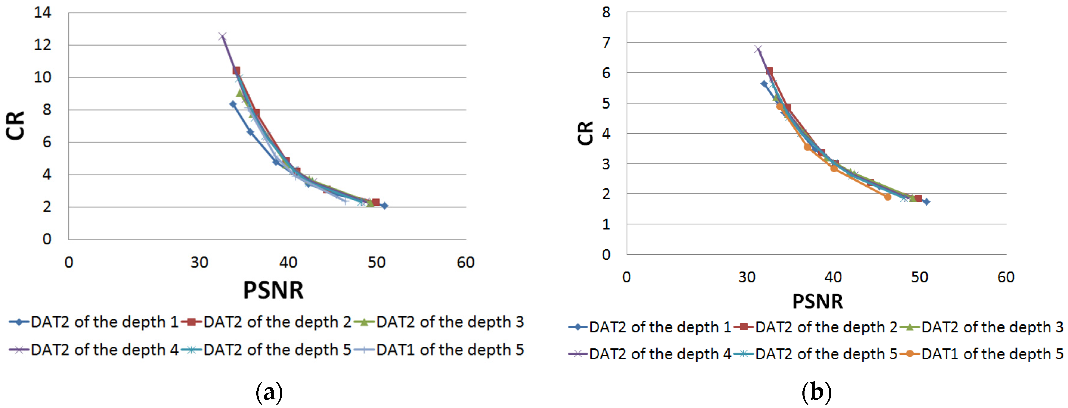
Next, in Figure 11, dependences of the mean value of CR on the mean value of PSNR for each structure of DAT are shown. We see that curves are close to each other except for the one corresponding to DAT2 of the depth 1. This means that it is not recommended to use DAT2 of the depth 1 and that a structure of DAT can be changed without significant changes of compression efficiency, which is important in the context of privacy protection requirements (see Section 2.2).

Finally, we verify the results presented above by processing other test data. In Figure 12, the test images SS3 and SS4 are shown.

Table 4. Results of compressing SS3 and SS4 using DAC with DAT1 of the depth 5.

Indicator	Image	UBMAD
		36	63	95	155
MAD	SS3	10	14	18	29
	SS4	8	14	20	41
RMSE	SS3	1.213	2.317	3.025	4.306
	SS4	1.222	2.498	3.604	5.198
PSNR, dB	SS3	46.451	40.832	38.518	35.449
	SS4	46.389	40.178	36.994	33.815
CR	SS3	2.347	3.906	5.134	8.103
	SS4	1.898	2.827	3.529	4.863

and

Table 5. Results of compressing SS3 and SS4 using DAC with DAT2 of the depth 2.

Indicator	Image	UBMAD
		7	14	20	25	46	64
MAD	SS3	5	9	12	15	27	34
	SS4	4	9	13	16	29	36
RMSE	SS3	0.814	1.536	2.270	2.617	3.869	4.949
	SS4	0.817	1.552	2.460	2.964	4.663	5.919
PSNR, dB	SS3	49.920	44.405	41.009	39.774	36.379	34.240
	SS4	49.889	44.311	40.312	38.694	34.757	32.687
CR	SS3	2.242	3.060	4.164	4.840	7.806	10.398
	SS4	1.836	2.363	2.987	3.343	4.830	6.047

contain results of their compressing. We stress that we have used the same quality loss settings as when processing the previous test data set. Figure 13 shows the dependence of CR on PSNR. It follows that there is no significant difference between results obtained for different structures of DAT. Furthermore, we see that indicators MAD, RMSE, PSNR, and CR belong to segments obtained when processing ESA images.

4. Considered Approach to Multichannel Image Classification

4.1. Maximum Likelihood Classifier

The process of pixel-by-pixel classification of raster images consists of the distribution of all pixels into classes in accordance with the value of each of them in one or more zones of the spectrum. Formally, the task is reduced to the creation of an optimal classifier that maps a set of observations of class attributes into a set of classes (represented by unique names or numbers) $d\left(x\right):X\to A$. The optimality criterion is usually understood as the requirement that when elements x from the observation space X are presented in the classification process, correct decisions are made as often as possible. Variability of spectral features, imperfect characteristics of imaging systems, noise, and interference during registration are sources of stochasticity in decision-making. Since observations X are realizations of random variables, the transformation d(x) is a random function, the class number also turns out to be a random variable. Thus, the design of pattern recognition methods is inevitably associated with the study of random mappings and is based on information-statistical methods for the formation of feature space, nonparametric estimation of probability densities, and the adoption of statistical hypotheses.

Statistical recognition methods, in contrast to heuristic ones, allow making mathematically sound decisions taking into account the available a priori information about the form of distribution$f\left(\overrightarrow{x};\overrightarrow{\theta }|a_k\right)$ for all sets of patterns $A=\left\{a_k\right\}$ and the probability of appearance of patterns for each class $P\left(a_k\right)$. In this case, the values of the attributes of the classes are considered as realizations of random variables, and their joint probability distribution densities are used to describe the etalons of the classes.

All statistical decision rules are based on the formation of the likelihood ratio L

$$\frac{f\left({\overrightarrow{x}}^{*};\overrightarrow{\theta }|a_u\right)}{f\left({\overrightarrow{x}}^{*};\overrightarrow{\theta }|a_v\right)}$$

and its comparison to a certain threshold, the value of which is determined by the selected criterion. The choice of criterion determines the way of dividing the space of features X into closed non-intersecting decision-making areas $G_k$, k = 1, 2, …, K, each of which contains such values of features $\overrightarrow{x}\in X$ that are most characteristic (probable) for one of the classes. Then, each pixel of the image s with spatial coordinates (i, j) is assigned to the class in the area of which its vector of values ${\overrightarrow{x}}^{*}\left(i,j\right)$ falls.

Complete and detailed knowledge of a priori information is consistent with the Bayesian approach to classification. The Bayesian classifier provides minimal error rates and is used to compare the performance of other classification algorithms. In the absence of information about the prior probabilities of classes and losses associated with making erroneous decisions, the maximum likelihood criterion is used. Following this criterion, the vector of values of a current pixel ${\overrightarrow{x}}^{*}\left(i,j\right)$ is alternately substituted into the probabilistic models of class etalons. The decision is made in favor of the class for which the likelihood function is maximal:

$$f\left({\overrightarrow{x}}^{*};\overrightarrow{\theta }|a_v\right)=\underset{1\le k\le K}{\max }\left\{f\left({\overrightarrow{x}}^{*};\overrightarrow{\theta }|a_k\right)\right\}\Rightarrow s\in a_v.$$

The results $f\left({\overrightarrow{x}}^{*}\left(i,j\right)|a_k\right)$, k = 1… K are compared to each other and the maximum value of the likelihood function is selected; its number is the number of the class to which the current pixel $s\left(i,j\right)$ belongs. Since, in statistical recognition, the densities $f\left(\overrightarrow{x};\overrightarrow{\theta }|a_k\right)$ are in general not known, their estimates obtained at the stage of training the classifier are substituted into the decision rule.

Supervised classification procedures (supervised learning) are characterized by the presence of training samples. When classifying remote sensing data, training samples are collections of pixels that represent a recognizable pattern or potential class. Usually, these are some well-defined homogeneous areas in the image, identified based on the true data on the Earth’s surface.

In the case of nonparametric estimation of the PDF based on the training sample (N points of the c-dimensional space), it is necessary to restore the form of the a priori unknown surface $f_c\left(\overrightarrow{x}\right)$ in the (c + 1)-dimensional space of features. Difficulties in constructing adequate multivariate statistical models are due to the fact that the methodology of data processing in the presence of correlations is based on the assumption that the distributions under consideration are normal. At the same time, the distributions of real multichannel data often have a non-Gaussian form and are determined over a finite interval of admissible values. To approximate such distributions, one can use the multivariate $S_B$–Johnson distribution

$$\begin{gathered} f_p\left(\overrightarrow{x}\right)={\left(2\pi \right)}^{-p/2}{\left|\mathbf{R}\right|}^{-1/2}{{\displaystyle \prod }}_{\kappa =1}^p\frac{{\eta }_{\kappa }{\lambda }_{\kappa }}{\left(x_{\kappa }-{\epsilon }_{\kappa }\right)\left({\lambda }_{\kappa }+{\epsilon }_{\kappa }-x_{\kappa }\right)}\times , \\ \times exp\left[-\frac{1}{2}{{\displaystyle \sum }}_{\kappa ,\upsilon =1}^p{R}_{\kappa \upsilon }^{-1}\left({\gamma }_{\kappa }+{\eta }_{\kappa }ln\left(\frac{x_{\kappa }-{\epsilon }_{\kappa }}{{\lambda }_{\kappa }+{\epsilon }_{\kappa }-x_{\kappa }}\right)\right)\left({\gamma }_{\upsilon }+{\eta }_{\upsilon }ln\left(\frac{x_{\upsilon }-{\epsilon }_{\upsilon }}{{\lambda }_{\upsilon }+{\epsilon }_{\upsilon }-x_{\upsilon }}\right)\right)\right], \end{gathered}$$

where ε is the displacement parameter, λ is the scale parameter, η and γ are the parameters of the distribution shape; R is a correlation matrix.

The disadvantage of the Johnson distribution is the lack of a direct connection between the estimates of sample moments with the distribution parameters $\overrightarrow{\theta }=\left\{\epsilon ,\lambda ,\eta ,\gamma \right\}$. Methods for estimating these parameters for each component of the feature vector are iterative and are reduced to solving an optimization problem of the form

$$\mathrm{F}\left(\overrightarrow{\theta }\right)={\displaystyle \int }{\left[H\left(x_{\kappa }\right)-f\left(x_{\kappa };\overrightarrow{\theta }\right)\right]}^{2}d{x}_{\kappa }\to min,$$

where $H\left(x_{\kappa }\right)$ is the empirical distribution (histogram) of the kth component.

Based on the results of constructing one-dimensional statistical models of the components of the feature vector for each class, it is possible to obtain a matrix of parameters of a multivariate distribution

$${\mathsf{\Theta }}_k={\left\{{\epsilon }_{\kappa k},{\lambda }_{\kappa k},{\eta }_{\kappa k},{\gamma }_{\kappa k}\right\}}_{p\times 4}.$$

The elements of the sample correlation matrix R are found as

$${\widehat{R}}_{\kappa \upsilon }=\frac{1}{NM}{{\displaystyle \sum }}_{i=1}^N{{\displaystyle \sum }}_{j=1}^M{z}_{\kappa }\left(i,j\right)z_{\upsilon }\left(i,j\right),$$

where z is a normal random variable with zero mathematical expectation and unit variance, obtained by transforming the original sample x:

$$z=\gamma +\eta ln\left(\frac{x-\epsilon }{\lambda +\epsilon -x}\right).$$

The obtained multidimensional models of class references are used to assign each analyzed pixel to a particular class based on the values of the likelihood functions.

4.2. ML Classifier Training

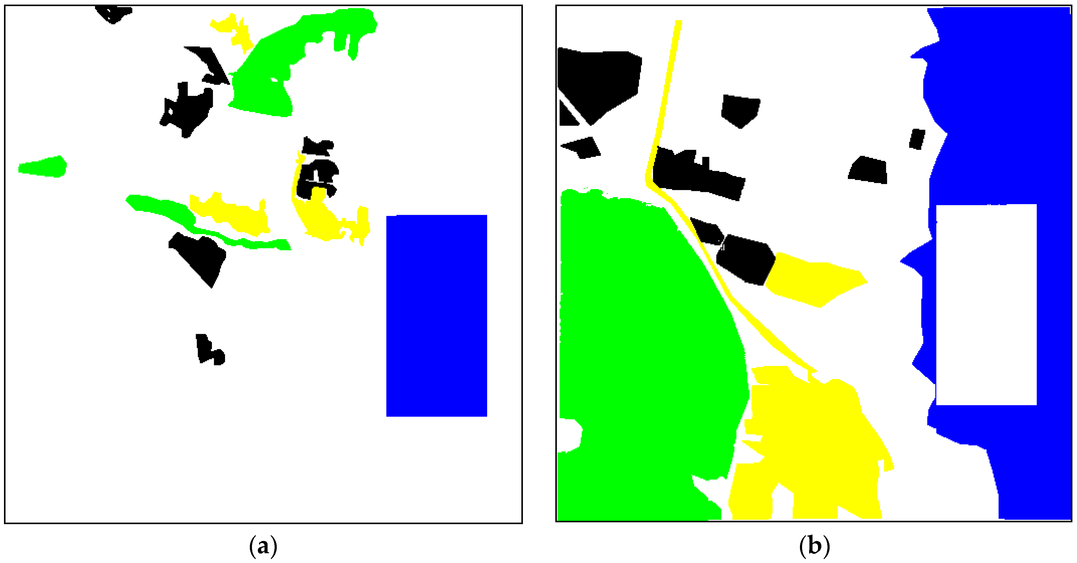
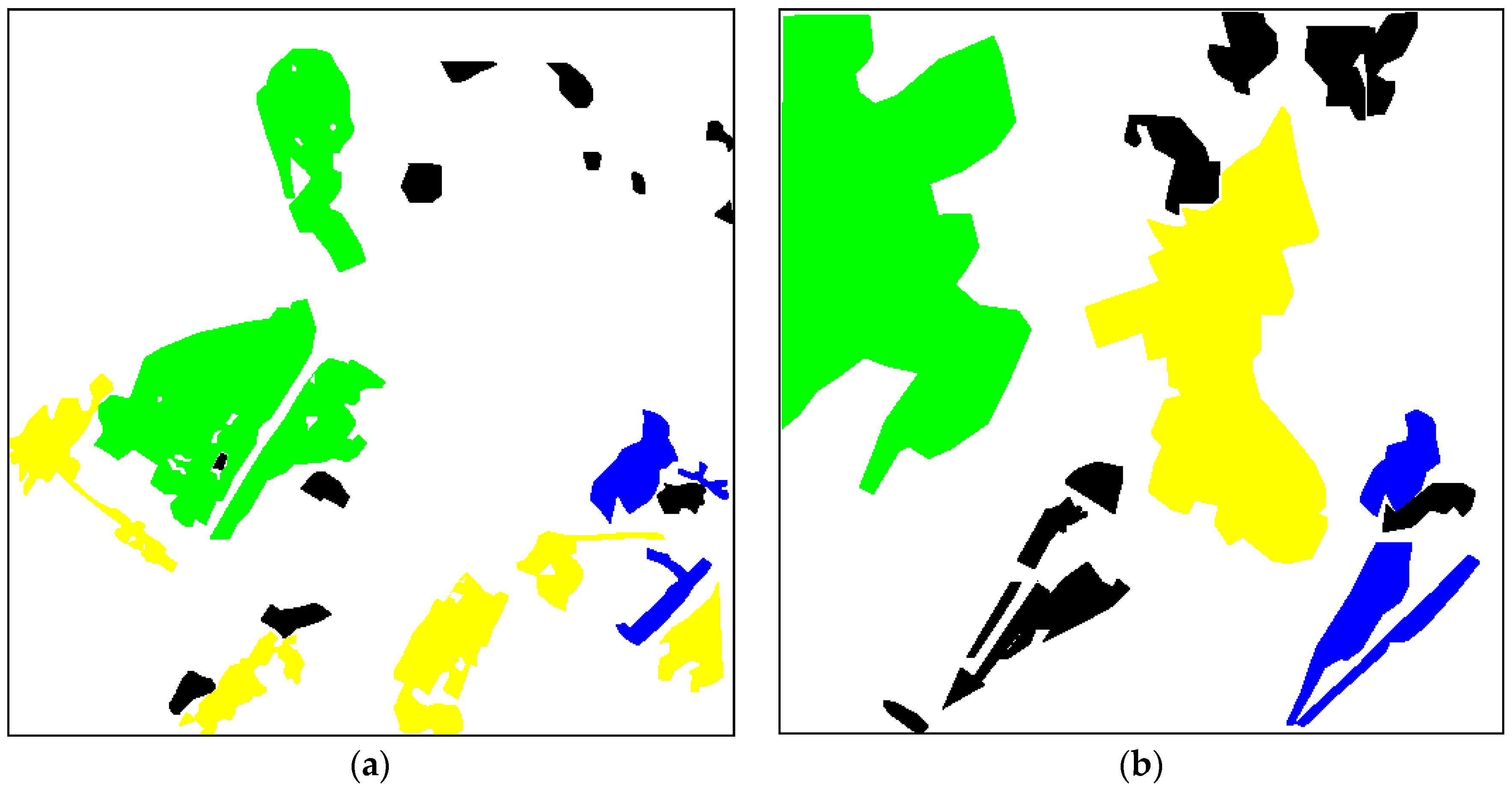
To study the effect of the compression procedure on the classification results, we have taken two multichannel images of 512 × 512 pixels obtained from the Sentinel-2 satellite (Figure 12). It has been assumed that each image contains four classes of objects: 1—Urban, 2—Water, 3—Vegetation, and 4—Bare soil. Based on factual data on the territory represented in these images (Kharkiv and its environs, Ukraine), relatively homogeneous fragments of images representing separate classes have been identified. Each of the selected fragments was marked with a conditional color corresponding to a certain class: Urban—yellow, Water—blue, Vegetation—green, and Bare soil—black. The sets of reference marked pixels have been divided into two non-overlapping subsets: training and control (verification) samples.

The marked areas (sets of reference pixels) have been divided into two subsets, which were used for training and assessing the quality of the classifier (Figure 14 and Figure 15). At the same time, it has been assumed that these subsets can partially overlap. The volumes of the training samples have been of the order of (4… 20) × 10³ pixels, the volumes of the verification samples have been several times larger ((7… 50) × 10³ pixels).

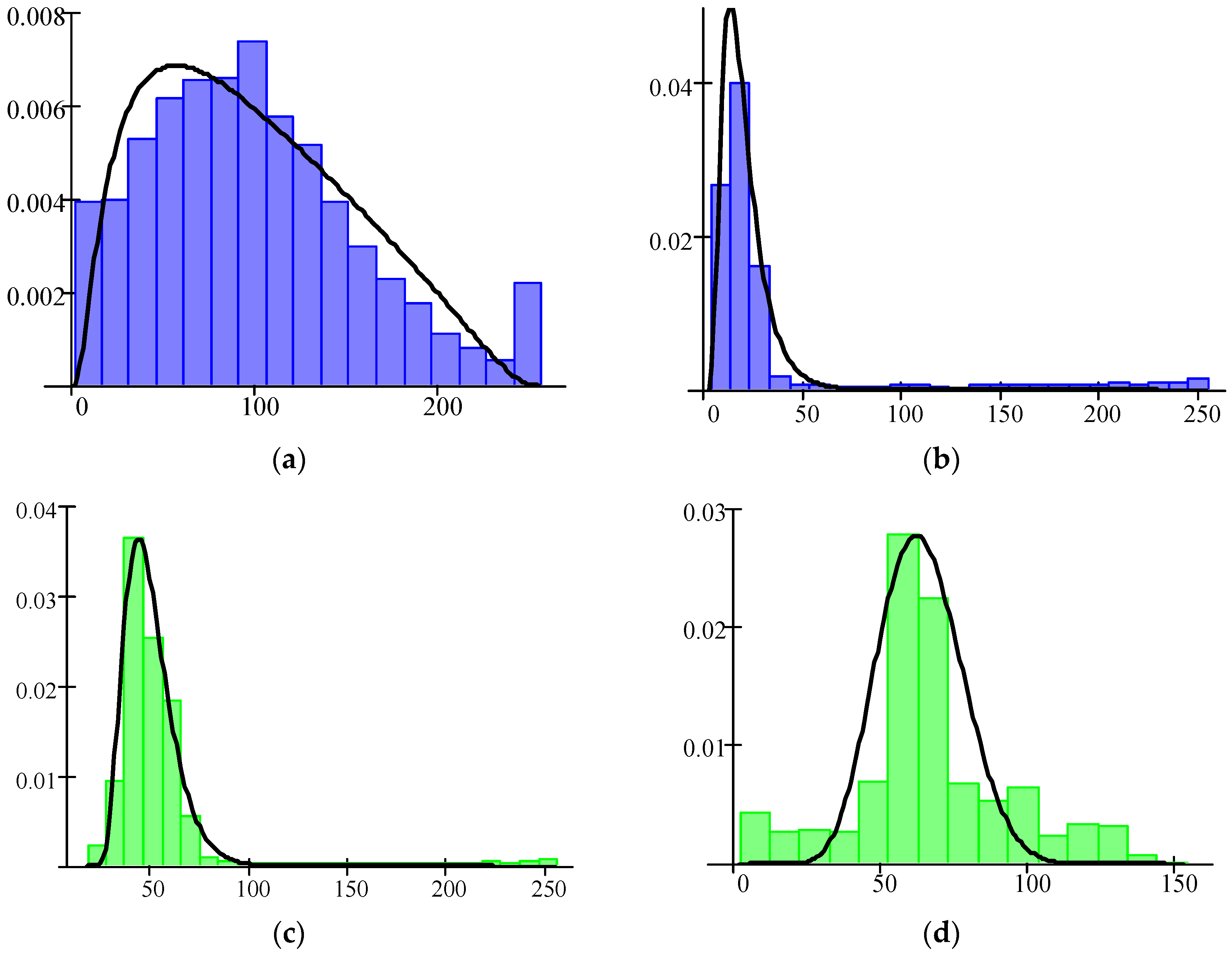
Figure 16 shows the empirical distributions of spectral features G, B for four classes of objects on the test image in Figure 12a, and graphs of the densities of Johnson’s S_B-distribution, which approximate them. As one can see, there is a sufficient overlapping of features in the feature space.

After obtaining the reference class descriptions, a pixel-by-pixel classification has been carried out according to the criterion of maximum likelihood. To assess the reliability of the classification, control samples have been used. The percentage of correctly recognized patterns of the kth class $Q_k$ was in this case an empirical estimate of the probability of correct recognition of the kth class $P_{kk}$. The estimate of the overall probability of correct recognition (quality criterion) for unknown (i.e., equiprobable) a priori class probabilities was determined as

$$P_{total}=\frac{1}{K}{{\displaystyle \sum }}_{k=1}^K{Q}_k.$$

5. Analysis of Classification Characteristics

Classification accuracy depends on many factors including a used classifier and its parameters, methodology of its training, image properties, and compression parameters. The classifier type, its parameters, and methodology of its training are fixed. Two images of different complexity will be analyzed in this Section. The main emphasis here is on the impact of compression parameters.

Let us start by considering the simpler structure image (Figure 12a). Let us analyze more in detail confusion matrices for compression with DAT of depth = 1 for different MAD values. The obtained results are presented in

Table 6. Probabilities of correct classifications for particular classes depending on image quality.

Class	Urban	Water	Vegetation	Bare Soil
	Original (Uncompressed) Image
Urban	0.912	1.71 × 10−4	5.05 × 10−3	0.083
Water	4.39 × 10−3	0.995	7.67 × 10−4	0
Vegetation	0.02	0.056	0.889	0.035
Bare soil	0.294	0	1.57 × 10−4	0.706
	Compressed image, MAD = 4
Urban	0.916	1.71 × 10−4	5.39 × 10−3	0.079
Water	0.018	0.972	0.011	0
Vegetation	0.02	0.051	0.902	0.026
Bare soil	0.31	0	7.85 × 10−5	0.690
	Compressed image, MAD = 7
Urban	0.921	1.28 × 10−4	5.05 × 10−3	0.074
Water	0.023	0.956	0.021	1.47 × 10−5
Vegetation	0.022	0.048	0.907	0.023
Bare soil	0.32	0	7.85 × 10−5	0.680
	Compressed image, MAD = 10
Urban	0.918	8.56 × 10−5	5.48 × 10−3	0.077
Water	0.027	0.954	0.019	2.95 × 10−5
Vegetation	0.022	0.046	0.91	0.022
Bare soil	0.338	0	2.36 × 10−4	0.661
	Compressed image, MAD = 16
Urban	0.918	1.71 × 10−4	6.04 × 10−3	0.076
Water	0.155	0.814	0.031	0
Vegetation	0.026	0.045	0.905	0.024
Bare soil	0.335	0	7.85 × 10−5	0.664
	Compressed image, MAD = 22
Urban	0.926	1.71 × 10−4	4.67 × 10−3	0.069
Water	0.035	0.945	0.020	0
Vegetation	0.025	0.039	0.925	0.011
Bare soil	0.295	0	0	0.705
	Compressed image, MAD = 35
Urban	0.915	2.14 × 10−4	6.76 × 10−3	0.078
Water	0.05	0.935	0.014	1.47 × 10−5
Vegetation	0.038	0.041	0.89	0.031
Bare soil	0.385	0	0	0.615

.

Analysis of data in Table 6 shows the following. First, classes are recognized with sufficiently different probabilities. The class Water is usually recognized in the best way although this is not the case for MAD = 16. Variations of the probability of correct recognition for the class Water (P₂₂) are due to two obstacles.

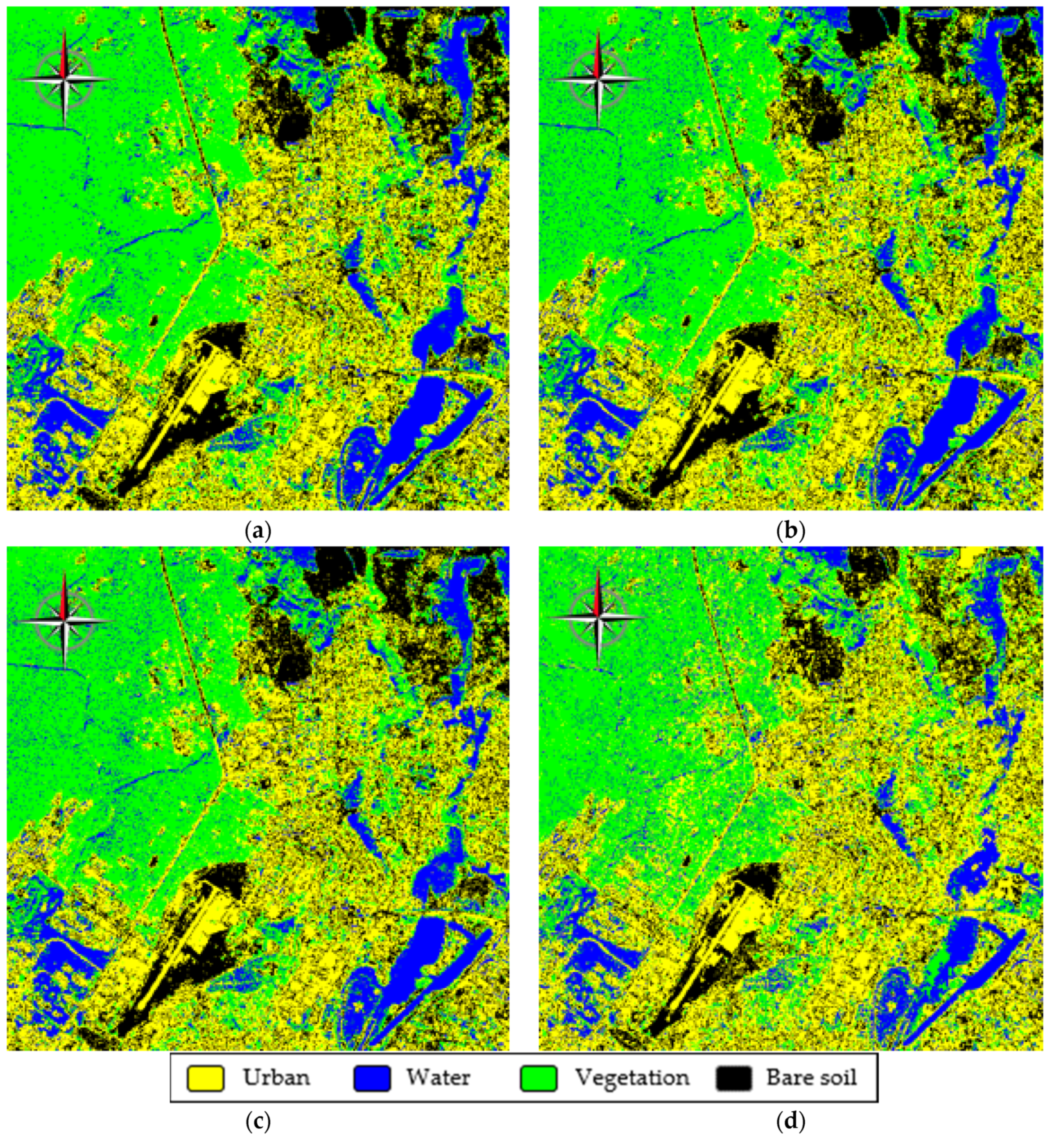
First, this class has sufficient overlapping of features distributions with other classes and probability density functions for this class are “narrow” (see Figure 17). Second, distortions due to lossy compression, in particular, mean shifting for large homogeneous areas, can lead to misclassifications. This effect is illustrated by two classification maps in Figure 18. For MAD = 16, there are many misclassifications (the pixels that belong to the class Water are related to the class Urban and shown by yellow color). The class Urban is recognized with approximately the same probability of correct recognition P₁₁. The probability of correct recognition P₃₃ for the class Vegetation does not change a lot. Finally, the probability of correct recognition P₄₄ for the class Bare Soil changes a little for small MAD values and sufficiently reduces for the largest MAD = 35.

Second, since there are overlappings in the feature space, there are misclassifications. In particular, the pixels belonging to the class Bare Soil are often recognized as Urban and vice versa. This is not surprising and always happens in RS data classification for classes “close” to each other.

Third, the total probability of correct classification P_total depends on MAD. Being equal to 0.876 for original images, it occurs to be equal to 0.87 for MAD = 4, 0.866 for MAD = 7, 0.861 for MAD = 10, 0.825 for MAD = 16, 0.875 for MAD = 22, and 0.839 for MAD = 35. Thus, there is some tendency of reduction of P_total with “local variations”.

Let us now consider the results for other depths of DAT. The obtained probabilities are presented in

Table 7. Probabilities for classes and total probabilities of correct classification for depth 2 and different MAD.

Classes	Depth_2
	MAD_5	MAD_9	MAD_12	MAD_15	MAD_27	MAD_34
Urban	0.917	0.919	0.919	0.919	0.916	0.917
Water	0.967	0.951	0.960	0.965	0.965	0.970
Vegetation	0.902	0.908	0.910	0.910	0.908	0.906
Bare soil	0.690	0.670	0.666	0.680	0.691	0.679
Ptotal	0.869	0.862	0.864	0.869	0.870	0.868

,

Table 8. Probabilities for classes and total probabilities of correct classification for depth 3 and different MAD.

Classes	Depth_3
	MAD_5	MAD_12	MAD_13	MAD_15	MAD_26	MAD_32
Urban	0.918	0.921	0.919	0.921	0.915	0.918
Water	0.963	0.954	0.955	0.958	0.964	0.936
Vegetation	0.905	0.908	0.909	0.905	0.895	0.895
Bare soil	0.689	0.659	0.663	0.650	0.667	0.649
Ptotal	0.869	0.861	0.862	0.859	0.860	0.850

,

Table 9. Probabilities for classes and total probabilities of correct classification for depth 4 and different MAD.

Classes	Depth_4
	MAD_5	MAD_11	MAD_14	MAD_20	MAD_29	MAD_42
Urban	0.917	0.919	0.919	0.918	0.918	0.917
Water	0.962	0.953	0.954	0.968	0.957	0.931
Vegetation	0.904	0.907	0.906	0.904	0.893	0.902
Bare soil	0.688	0.659	0.657	0.663	0.663	0.648
Ptotal	0.868	0.860	0.859	0.863	0.858	0.850

and

Table 10. Probabilities for classes and total probabilities of correct classification for depth 5 and different MAD.

Classes	Depth_5
	MAD_6	MAD_11	MAD_13	MAD_21	MAD_27	MAD_35
Urban	0.917	0.919	0.921	0.919	0.919	0.916
Water	0.964	0.954	0.954	0.966	0.966	0.975
Vegetation	0.904	0.906	0.906	0.902	0.895	0.896
Bare soil	0.681	0.651	0.650	0.674	0.666	0.665
Ptotal	0.866	0.857	0.858	0.865	0.862	0.863

.

As one can see, probabilities for particular classes slightly vary depending on the depth of DAT and MAD but not by much. They remain more stable than in the case of DAT with depth 1. Concerning the total probability of correct classification, its small degradation with MAD increasing is observed for depths 3 and 4, but reduction can be considered acceptable, if it does not exceed 0.02.

Let us now consider the second real-life test image that has a complex structure (Figure 12b). Its classification maps for the original image and three values of MAD are presented in Figure 19. The comparison shows that there are no essential differences between the classification maps. Another observation is that there are quite many misclassifications from the Vegetation class to Water (authors from Kharkiv live or work in this region). The confusion matrix (

Table 11. Confusion matrix for original image in Figure 12b.

Class	Probability of Decision
	Urban	Water	Vegetation	Bare Soil
Urban	0.645	2.9 × 10−2	9.6 × 10−2	0.230
Water	4.3 × 10−2	0.860	8.7 × 10−2	9.7 × 10−3
Vegetation	4.87 × 10−3	0.052	0.943	1.8 × 10−4
Bare soil	0.160	7.54 × 10−3	3.8 × 10−2	0.795

) confirms this. Here, it is seen that the class Water is recognized worse than in the previous case. The class Urban is also recognized worse while the classes Vegetation and Bare Soil are recognized better than in the previous case. P_total equals 0.811. For comparison,

Table 12. Confusion matrix for the image compressed with DAT of depth 1 with MAD = 11.

Class	Probability of Decision
	Urban	Water	Vegetation	Bare Soil
Urban	0.647	0.0249	0.0975	0.2307
Water	0.0534	0.8236	0.1132	9.84 × 10−3
Vegetation	8.71 × 10−3	0.0911	0.90	2.32 × 10−4
Bare soil	0.1729	6.47 × 10−3	0.0425	0.7781

gives an example of a confusion matrix for the compressed image. As one can see, there is no essential difference, at least in probabilities P₁₁, P₂₂, P₃₃, and P₄₄. P_total = 0.787, i.e., noticeable reduction of P_total takes place, and it is worth analyzing probabilities for different MAD values and depths of DAT.

Thus, let us consider data for different depths of DAT and different values of MAD. They are presented in

Table 13. Probabilities for classes and total probabilities of correct classification for depth 1 and different MAD.

Classes	Depth_1
	MAD_4	MAD_7	MAD_11	MAD_16	MAD_25	MAD_34
Urban	0.6469	0.6483	0.6469	0.6488	0.6565	0.6733
Water	0.8424	0.8316	0.8236	0.8201	0.8428	0.6991
Vegetation	0.9058	0.8938	0.9	0.8994	0.8797	0.865
Bare soil	0.7964	0.7849	0.7781	0.7652	0.7526	0.6035
Ptotal	0.798	0.790	0.787	0.783	0.783	0.710

,

Table 14. Probabilities for classes and total probabilities of correct classification for depth 2 and different MAD.

Classes	Depth_2
	MAD_4	MAD_9	MAD_13	MAD_16	MAD_29	MAD_36
Urban	0.6476	0.6471	0.6479	0.6479	0.6536	0.6603
Water	0.8409	0.8287	0.8247	0.8232	0.8282	0.829
Vegetation	0.9027	0.8952	0.9012	0.8999	0.8951	0.9016
Bare soil	0.7915	0.7827	0.7729	0.7763	0.7844	0.7799
Ptotal	0.796	0.788	0.787	0.787	0.790	0.793

,

Table 15. Probabilities for classes and total probabilities of correct classification for depth 3 and different MAD.

Classes	Depth_3
	MAD_5	MAD_10	MAD_14	MAD_15	MAD_30	MAD_40
Urban	0.6482	0.6459	0.6462	0.647	0.654	0.6528
Water	0.835	0.8246	0.823	0.8237	0.8139	0.8036
Vegetation	0.8997	0.8992	0.9002	0.8996	0.888	0.9109
Bare soil	0.794	0.7809	0.7781	0.7657	0.7651	0.7819
Ptotal	0.794	0.788	0.787	0.784	0.780	0.787

,

Table 16. Probabilities for classes and total probabilities of correct classification for depth 4 and different MAD.

Classes	Depth_4
	MAD_6	MAD_12	MAD_15	MAD_21	MAD_30	MAD_44
Urban	0.6482	0.6481	0.6501	0.6496	0.6545	0.6707
Water	0.8358	0.8247	0.8204	0.8154	0.8189	0.7712
Vegetation	0.8912	0.8969	0.8975	0.8949	0.886	0.8866
Bare soil	0.7923	0.7759	0.7646	0.7661	0.7775	0.7498
Ptotal	0.792	0.786	0.783	0.782	0.784	0.770

and

Table 17. Probabilities for classes and total probabilities of correct classification for depth 5 and different MAD.

Classes	Depth_5
	MAD_7	MAD_11	MAD_15	MAD_22	MAD_32	MAD_35
Urban	0.6496	0.6489	0.6505	0.6521	0.6528	0.6668
Water	0.8431	0.83	0.8255	0.8121	0.7986	0.8079
Vegetation	0.9021	0.9017	0.8995	0.8903	0.8854	0.8949
Bare soil	0.7912	0.77	0.7618	0.7704	0.7694	0.7598
Ptotal	0.797	0.788	0.784	0.781	0.777	0.782

. As it follows from data analysis in these Tables, there is a tendency of reduction of P_total if MAD increases. This is especially obvious for a depth equal to 1. For MAD = 34, the considerable reduction of P₂₂ and P₄₄ takes place.

The smallest reduction takes place for depth = 2. For other depths, the results for depths 3, 4, and 5 are, in general, better than for depth = 1, but worse than for depth = 2. For depth = 2, it is possible to state that classification results are acceptable for all considered MAD values (even MAD = 36) because P_total for compressed images is less than P_total for the original image by no more than 0.03.

Certainly, these two examples are not enough to obtain full imagination of classification accuracy of compressed images and give some final recommendations. Besides, classification results usually depend on a classifier applied. To partly move around these shortcomings of previous analysis, we have carried out additional experiments for other Sentinel-2 images of different complexity, the Landsat image, and a neural network classifier. The obtained data are briefly presented below (a more detailed data can be found at the following link to the Google drive folder: https://drive.google.com/drive/folders/14m7TLLM7o836yGzJo9NKlaUc9sLsL5VK?usp=sharing, accessed on 27 October 2021).

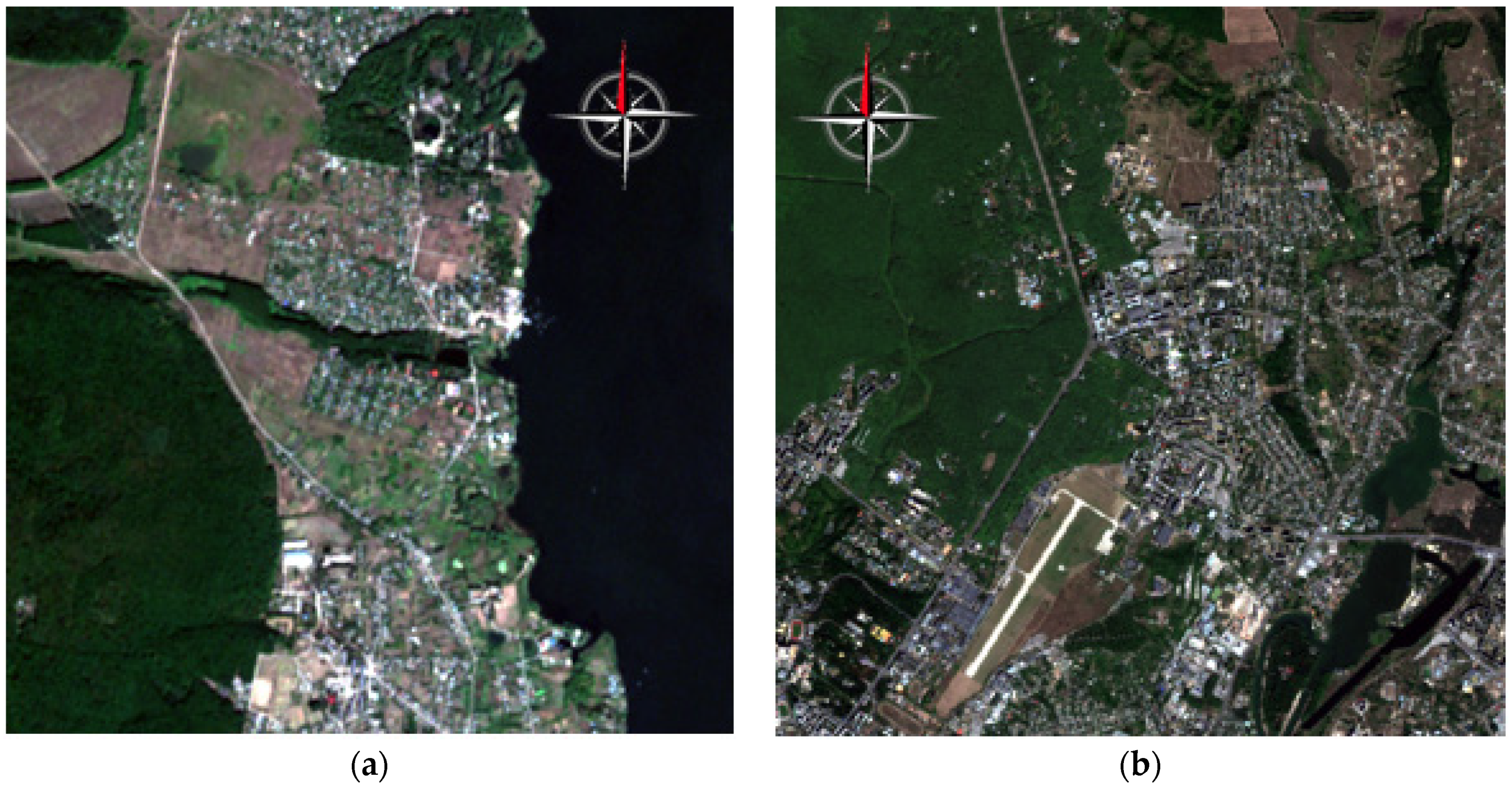
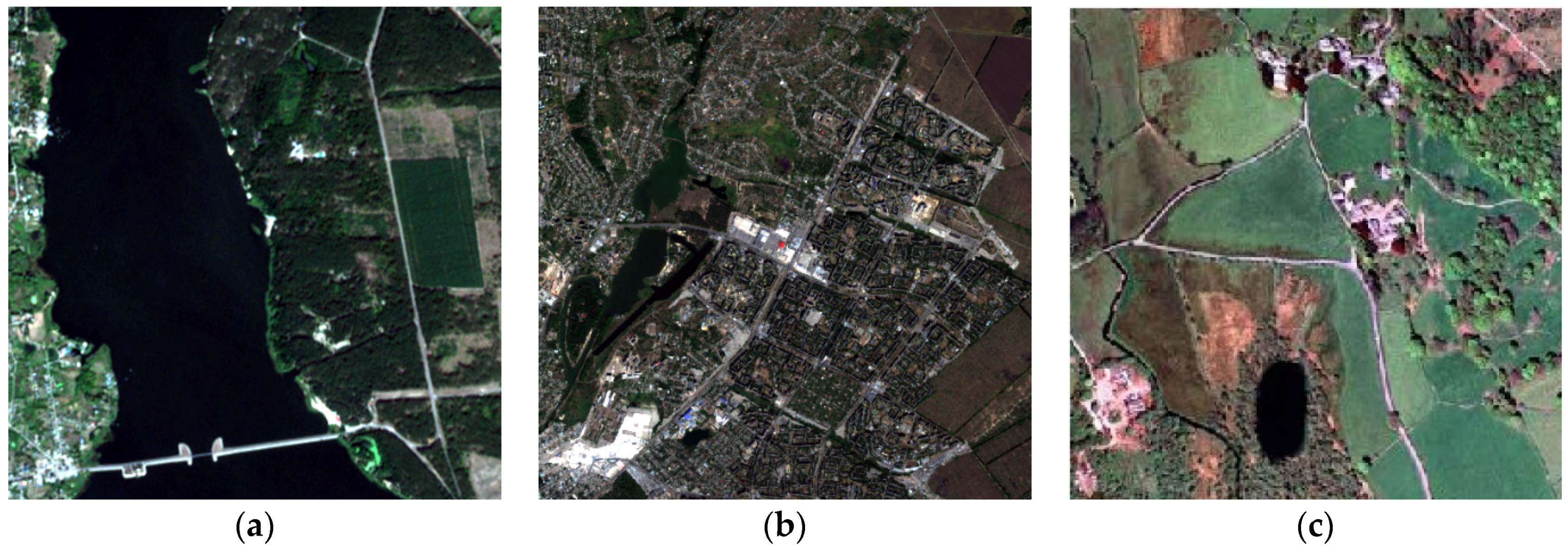
The experiments have been performed for 512 × 512 pixel fragments of Sentinel-2 and Landsat images (Figure 20).

Table 18. Total probabilities of correct classification for depth 2 and different MAD for the image in Figure 20a using ML and NN classifiers.

Classifier	Depth_2
	MAD_5	MAD_9	MAD_12	MAD_15	MAD_27	MAD_34
ML	0.869	0.862	0.864	0.869	0.870	0.862
NN	0.878	0.873	0.875	0.880	0.877	0.871

presents the total probabilities of correct classification for the image in Figure 20, a compressed with depth 2. The three-layer neural network (NN) classifier has been trained using the same fragments as for the ML classifier. The verification fragments are also the same to provide the correctness of comparisons. Classifiers have been trained for non-compressed data. The analysis shows that the probabilities are practically at the same level for all MAD values except the last one where a small reduction of P_total is observed. The classification accuracy for the NN classifier is slightly better but not sufficiently.

Table 19. Total probabilities of correct classification for depth 2 and different MAD for the image in Figure 20b using ML and NN classifiers.

Classifier	Depth_2
	MAD_5	MAD_9	MAD_13	MAD_17	MAD_30	MAD_39
ML	0.842	0.836	0.827	0.829	0.821	0.814
NN	0.862	0.850	0.849	0.846	0.846	0.837

gives the results (P_total) for the image in Figure 20b. As one can see, the more complicated structure image is classified worse than a simpler one (compare the data in Table 18 and Table 19). Again, the NN classifier performs a little bit better than the ML one. Finally, there is a general tendency to reduction of P_total if the MAD of introduced losses increases. Meanwhile, if MAD is less than 30, the reduction of classification accuracy is acceptable.

Finally,

Table 20. Total probabilities of correct classification for depth 2 and different MAD for the image in Figure 20c using the ML classifier.

Classes	Original	MAD_4	MAD_7	MAD_11	MAD_18	MAD_24	MAD_37
Soil	0.747	0.740	0.741	0.744	0.736	0.695	0.651
Grass	0.812	0.810	0.811	0.810	0.796	0.798	0.343
Water	0.967	0.967	0.970	0.970	0.968	0.967	0.974
Urban	0.989	0.989	0.989	0.989	0.986	0.985	0.982
Bushes	0.812	0.805	0.806	0.807	0.797	0.718	0.701
Ptotal	0.865	0.862	0.863	0.864	0.857	0.833	0.730

presents a part of the results obtained for the Landsat image in Figure 20c using the ML classifier. The probabilities for particular five classes and the total probability of correct classification are given. As one can see, the classification results are quite stable if introduced distortions are not too large (MAD < 20, PSNR > 38 dB), then a fast reduction of classification accuracy takes place if MAD increases (PSNR decreases).

In addition, in Figure 21, the results of compressing the images given in Figure 20 are presented. Figure 21a shows almost the same behavior of dependence of PSNR on MAD for all three images. This means that the dependence of PSNR on MAD depends on image content only slightly. In contrast, compression efficiency measured by CR significantly depends on the image content. For instance, the test image shown in Figure 20b has a lot of small objects and sharp changes of color intensity. As one can see, CR for this image is the smallest for any value of PSNR considered (Figure 21b).

6. Discussion

Below, we discuss the obtained results and present some recommendations concerning their further applications.

First, computation complexity is of particular interest, especially, when processing a huge amount of digital images. In [54], it has been shown that computation of DAT-coefficients is linear in the size of data processed, i.e., time complexity of DAT is O(N), where N is the number of pixels. However, one specific feature of digital devices and/or computational systems should be taken into account when applying DAC. In terms of time expenses, data transferring from one memory part to another (needed in the calculation of DAT) can take more time than performing arithmetic operations [56]. Note that when applying DAT of the depth greater than 1, such a transferring is used and the time needed for it increases if depth becomes larger. For this reason, the use of DAT of the low depth can be recommended if high performance is required.

Second, it follows from the results obtained in the previous sections that DAT2 of the depth 2 can be recommended from the viewpoint of the same performance compared to DAT versions with the larger depth. Since this recommendation is consistent with the observation for computational complexity, the use of DAT2 with depth = 2 can be treated as a reasonable practical choice.

In practice, one might need to provide lossy compression of RS data with providing the desired quality characterized, e.g., by the desired PSNR. In this sense, although inequalities (7) and (12) are upper estimates, there is a possibility to obtain compressed data with loss of quality measured by PSNR, MAD, or RMSE which are close to the desired values. Consider this, e.g., for PSNR. Let a structure of DAT be fixed. For instance, let DAT1 of the depth 5 or DAT2 of the depth 2 be chosen. If PSNR = p is desired, then settings of DAC can be found as follows:

–

compute $\mathrm{RMSE}=\mathrm{r}=255·{10}^{-\mathrm{p}/20}$;

–

find MAD = $(\mathrm{r}-\mathrm{b})/\mathrm{a}$, where a and b are parameters of linear regression $\mathrm{y}=\mathrm{a}\mathrm{x}+\mathrm{b}$, $\mathrm{x}=\mathrm{M}\mathrm{A}\mathrm{D}$, $\mathrm{y}=\mathrm{RMSE}$ (here, the values presented in Table 1 can be used);

–

find UBMAD, using interpolation methods and data from Table 2 or Table 3 depending on the structure of DAT.

The value of UBMAD computed defines the settings of DAC. These settings provide distortions measured by PSNR that, with high probability, belong to an appropriately narrow neighborhood of p.

The UBMAD can be also found directly, using the dependence of the mean value of PSNR on UBMAD (see data in Table 2 and Table 3). However, the error of providing a desired PSNR might be greater due to non-linear dependence between these two parameters if linear interpolation is applied.

In addition, as is mentioned in Section 2.1, any matrix M can be processed by DAT of arbitrary structure. Although, in this case, if its rows or columns do not satisfy the length condition mentioned, then application of the extension procedure is required. This leads to an increase in the number of DAT coefficients. Nevertheless, since atomic wavelets have zero mean value [57], most extra DAT coefficients are equal to zero. Such data are well compressed by the proposed coding. When processing images of a high resolution, a wide variety of the DAT variants can be applied without a significant increase of additional data. Moreover, if the DAC is considered as a data protection coder, then some increase in the compressed file size is insignificant.

Besides, it is shown that there is no significant difference in the mean value of CR provided by DAT1 and DAT2 (except the case of the depth 1) for any distortions measured by PSNR (see Figure 11). This means that significant variation of the structure of DAT does not affect significant changes in compression efficiency. Such a result provides the possibility to achieve both compression and protection.

Finally, the algorithm DAC was compared with JPEG in [40,41,47]. It has been shown that, on average, DAC provides a higher compression ratio than JPEG for the same quality measured by PSNR. We note that previously Huffman codes and run-length encoding were used to compress quantized DAT-coefficients. In the current research, binary arithmetic coding is applied instead. In [65], it has been shown that such an approach provides better compression of quantized DAT-coefficients than a combination of Huffman codes with run-length encoding. Hence, the following statement is valid: on average, the algorithm DAC with binary arithmetic coding of quantized DAT-coefficients compresses three-channel better than JPEG with the same distortions measured by PSNR.

Furthermore, the proposed quality loss control mechanism provides distortions measured by MAD that are not greater than UBMAD, which defines quality loss settings. It is only this value that can be varied to obtain different quality losses. In Section 3, using statistical methods, it is shown that there is linear dependence of RMSE on MAD, and coefficients of linear regression are provided. Hence, a mechanism for controlling the loss of quality measured by RMSE and PSNR is obtained. This result is of particular importance since the metric MAD is adequate only if it is small; other metrics, especially RMSE and PSNR should be used otherwise. Further, inequality MAD $\le$UBMAD is an upper bound. If the value of UBMAD is fixed, then actual MAD can be significantly smaller than UBMAD. This feature is shown in Table 2 and Table 3. Nevertheless, in these tables, the dependence of the mean value of MAD (also, RMSE, PSNR, and CR) and its deviation on UBMAD is provided. Moreover, it is shown that a high percentage of values obtained experimentally belongs to segments [E − $2\mathsf{\sigma }$, E + $2\mathsf{\sigma }$], where E is the mean value and $\mathsf{\sigma }$ is deviation. In other words, the limits of efficiency indicators are obtained for each structure of DAT and each value of UBMAD. This provides a possibility to obtain the desired results in terms of MAD, RMSE, PSNR, and CR.

Finally, we have carried out verification of the proposed approach for some other three-channel images acquired by Sentinel-2 and then compressed by DAT2 with depth equal to 2. The obtained results and recommendations are similar to those presented for the two images used in our research above.

In the future for additional assessment of quality and accuracy of the proposed methods, it will be useful to deal with more sensitive classification tasks such as different crop type classification and other applied problems.

7. Conclusions

In this paper, we have analyzed the task of lossy compression of three-channel images using discrete atomic transform. Two real-life images of different complexity have been considered. The quality of compressed images has been characterized in different ways: using MAD and RMSE (or PSNR) and applying probabilities of correct recognition, both total and for particular classes (ML classifiers have been used).

The following has been demonstrated:

-

There are many versions of DAC where compression using DAT2 with depth equal to 2 can be recommended for practical use because of the following reasons: (a) it has quite low computational complexity; (b) rate/distortion characteristics are better than for DAC with DAT of depth 1 and practically the same as for DAT with larger depth values; (c) privacy protection is provided; taken all together, these properties explain our recommendation.

-

Lossy compression based on DAT is controlled by UBMAD but we have got approximations that allow recalculating UPMAD to MAD, RMSE, and PSNR and, thus, providing the desired quality of compressed images quite accurately and without iterations; this is a useful property especially if compression should be performed quickly, e.g., onboard of satellite or airborne carrier with compressing large volumes of RS data;

-

classification results (obtained for ML classifier) for lossy compressed data depend on image complexity; for the image of low complexity, lossy compression has a low negative impact on classification accuracy if MAD is less than 35 (PSNR is larger than about 34 dB); for the image of high complexity, lossy compression for the same conditions might lead to a reduction of total probability of correct classification by about 3% that seems to be acceptable for practice.

-

DAT-based compression performs better than JPEG, and one of its main advantages is the possibility of easily providing data privacy.

In the future, we plan to analyze more images and consider other classifiers; besides, we plan to extend the DAT-based compression to RS data with more than three numbers of channels and other applied tasks such as crop type classification monitoring of forests cuts, etc.

References

1. Pillai, D.K. New Computational Models for Image Remote Sensing and Big Data. In Big Data Analytics for Satellite Image Processing and Remote Sensing; Swarnalatha, P., Sevugan, P., Eds.; IGI Global: Hershey, PA, USA, 2018; pp. 1–21. [Google Scholar]
2. Mielke, C.; Boshce, N.K.; Rogass, C.; Segl, K.; Gauert, C.; Kaufmann, H. Potential Applications of the Sentinel-2 Multispectral Sensor and the ENMAP hyperspectral Sensor in Mineral Exploration. EARSeL Eproc. 2014, 13, 93–102. [Google Scholar] [CrossRef]
3. Joshi, N.; Baumann, M.; Ehammer, A.; Fensholt, R.; Grogan, K.; Hostert, P.; Jepsen, M.R.; Kuemmerle, T.; Meyfroidt, P.; Mitchard, E.T.A.; et al. A Review of the Application of Optical and Radar Remote Sensing Data Fusion to Land Use Mapping and Monitoring. Remote Sens. 2016, 8, 70. [Google Scholar] [CrossRef] [Green Version]
4. Kussul, N.; Lavreniuk, M.; Kolotii, A.; Skakun, S.; Rakoid, O.; Shumilo, L. A workflow for Sustainable Development Goals indicators assessment based on high-resolution satellite data. Int. J. Digit. Earth 2020, 13, 309–321. [Google Scholar] [CrossRef]
5. Kolotii, A.; Kussul, N.; Shelestov, A.; Skakun, S.; Yailymov, B.; Basarab, R.; Ostapenko, V. Comparison of biophysical and satellite predictors for wheat yield forecasting in Ukraine. Int. Arch. Photogramm. Remote Sens. Spat. Inf. Sci.—ISPRS Arch. 2015, 40, 39–44. [Google Scholar] [CrossRef] [Green Version]
6. Kussul, N.; Mykola, L.; Shelestov, A.; Skakun, S. Crop inventory at regional scale in Ukraine: Developing in season and end of season crop maps with multi-temporal optical and SAR satellite imagery. Eur. J. Remote Sens. 2018, 51, 627–636. [Google Scholar] [CrossRef] [Green Version]
7. Kussul, N.; Shelestov, A.; Lavreniuk, M.; Butko, I.; Skakun, S. Deep learning approach for large scale land cover mapping based on remote sensing data fusion. In Proceedings of the 2016 IEEE International Geoscience and Remote Sensing Symposium (IGARSS), Beijing, China, 10–15 July 2016; pp. 198–201. [Google Scholar] [CrossRef]
8. Zhong, P.; Wang, R. Multiple-Spectral-Band CRFs for Denoising Junk Bands of Hyperspectral Imagery. IEEE Trans. Geosci. Remote Sens. 2013, 51, 2269–2275. [Google Scholar] [CrossRef]
9. Sajjad, H.; Kumar, P. Future Challenges and Perspective of Remote Sensing Technology. In Applications and Challenges of Geospatial Technology; Kumar, P., Rani, M., Chandra Pandey, P., Sajjad, H., Chaudhary, B., Eds.; Springer: Cham, Switzerland, 2019; pp. 275–277. [Google Scholar] [CrossRef]
10. First Applications from Sentinel-2A. Available online: http://www.esa.int/Our_Activities/Observing_the_Earth/Copernicus/Sentinel-2/First_applications_from_Sentinel-2A (accessed on 7 October 2021).
11. Kussul, N.; Lemoine, G.; Gallego, F.J.; Skakun, S.; Lavreniuk, M.; Shelestov, A. Parcel-Based Crop Classification in Ukraine Using Landsat-8 Data and Sentinel-1A Data. IEEE J. Sel. Top. Appl. Earth Obs. Remote Sens. 2016, 9, 2500–2508. [Google Scholar] [CrossRef]
12. Bioucas-Dias, J.M.; Plaza, A.; Camps-Valls, G.; Scheunders, P.; Nasrabadi, N.; Chanussot, J. Hyperspectral Remote Sensing Data Analysis and Future Challenges. IEEE Geosci. Remote Sens. Mag. 2013, 1, 6–36. [Google Scholar] [CrossRef] [Green Version]
13. Chi, M.; Plaza, A.; Benediktsson, J.A.; Sun, Z.; Shen, J.; Zhu, Y. Big Data for Remote Sensing: Challenges and Opportunities. Proc. IEEE 2016, 104, 2207–2219. [Google Scholar] [CrossRef]
14. Manolakis, D.G.; Lockwood, R.B.; Cooley, T.W. Hyperspectral Imaging Remote Sensing: Physics, Sensors, and Algorithms; Cambridge University Press: Cambridge, UK, 2016. [Google Scholar] [CrossRef]
15. Yu, G.; Vladimirova, T.; Sweeting, M.N. Image compression systems on board satellites. Acta Astronaut. 2009, 64, 988–1005. [Google Scholar] [CrossRef]
16. Christophe, E. Hyperspectral Data Compression Tradeoff. In Optical Remote Sensing in Advances in Signal Processing and Exploitation Techniques; Prasad, S., Bruce, L., Chanussot, J., Eds.; Springer: Berlin/Heidelberg, Germany, 2011; pp. 9–29. [Google Scholar] [CrossRef]
17. Blanes, I.; Magli, E.; Serra-Sagrista, J. A Tutorial on Image Compression for Optical Space Imaging Systems. IEEE Geosci. Remote Sens. Mag. 2014, 2, 8–26. [Google Scholar] [CrossRef] [Green Version]
18. Zemliachenko, A.N.; Kozhemiakin, R.A.; Uss, M.L.; Abramov, S.K.; Ponomarenko, N.N.; Lukin, V.V. Lossy compression of hyperspectral images based on noise parameters estimation and variance stabilizing transform. J. Appl. Remote Sens. 2014, 8, 25. [Google Scholar] [CrossRef]
19. Chow, K.; Tzamarias, D.E.O.; Blanes, I.; Serra-Sagristà, J. Using Predictive and Differential Methods with K2-Raster Compact Data Structure for Hyperspectral Image Lossless Compression. Remote Sens. 2019, 11, 2461. [Google Scholar] [CrossRef] [Green Version]
20. Radosavljevic, M.; Brkljac, B.; Lugonja, P.; Crnojevic, V.; Trpovski, Ž.; Xiong, Z.; Vukobratovic, D. Lossy Compression of Multispectral Satellite Images with Application to Crop Thematic Mapping: A HEVC Comparative Study. Remote Sens. 2020, 12, 1590. [Google Scholar] [CrossRef]
21. Blanes, I.; Kiely, A.; Hernández-Cabronero, M.; Serra-Sagristà, J. Performance Impact of Parameter Tuning on the CCSDS-123.0-B-2 Low-Complexity Lossless and Near-Lossless Multispectral and Hyperspectral Image Compression Standard. Remote Sens. 2019, 11, 1390. [Google Scholar] [CrossRef] [Green Version]
22. Aiazzi, B.; Alparone, L.; Baronti, S. Near-lossless compression of 3-D optical data. IEEE Trans. Geosci. Remote Sens. 2001, 39, 2547–2557. [Google Scholar] [CrossRef]
23. Aiazzi, B.; Alparone, L.; Baronti, S.; Lastri, C.; Selva, M. Spectral Distortion in Lossy Compression of Hyperspectral Data. J. Electr. Comput. Eng. 2012, 2012, 850637. [Google Scholar] [CrossRef] [Green Version]
24. Santos, L.; Lopez, S.; Callico, G.; Lopez, J.; Sarmiento, R. Performance evaluation of the H.264/AVC video coding standard for lossy hyperspectral image compression. IEEE J. Sel. Top. Appl. Earth Observ. Remote Sens. 2012, 5, 451–461. [Google Scholar] [CrossRef]
25. Krivenko, S.; Krylova, O.; Bataeva, E.; Lukin, V. Smart Lossy Compression of Images Based on Distortion Prediction. Telecommun. Radio Eng. 2018, 77, 1535–1554. [Google Scholar] [CrossRef]
26. Vasilyeva, I.; Li, F.; Abramov, S.; Lukin, V.V.; Vozel, B.; Chehdi, K. Lossy compression of three-channel remote sensing images with controllable quality. In Proceedings of the SPIE 11862, Image and Signal Processing for Remote Sensing XXVII, Madrid, Spain, Online Only. 12 September 2021; p. 118620R. [Google Scholar] [CrossRef]
27. Penna, B.; Tillo, T.; Magli, E.; Olmo, G. Transform Coding Techniques for Lossy Hyperspectral Data Compression. IEEE Trans. Geosci. Remote Sens. 2007, 45, 1408–1421. [Google Scholar] [CrossRef]
28. Manolakis, D.; Lockwood, R.; Cooley, T. On the Spectral Correlation Structure of Hyperspectral Imaging Data. In Proceedings of the IGARSS 2008—2008 IEEE International Geoscience and Remote Sensing Symposium, Boston, MA, USA, 7–11 July 2008; pp. II-581–II-584. [Google Scholar]
29. Lam, K.W.; Lau, W.; Li, Z. The effects on image classification using image compression technique. Amsterdam. Int. Arch. Photogramm. Remote Sens. 2000, 33, 744–751. [Google Scholar]
30. Ozah, N.; Kolokolova, A. Compression improves image classification accuracy. In Advances in Artificial Intelligence. Canadian AI 2019. Lecture Notes in Computer Science; Meurs, M.J., Rudzics, F., Eds.; Springer: Cham, Switzerland, 2019; pp. 525–530. [Google Scholar] [CrossRef]
31. Chen, Z.; Ye, H.; Yingxue, Z. Effects of Compression on Remote Sensing Image Classification Based on Fractal Analysis. IEEE Trans. Geosci. Remote Sens. 2019, 57, 4577–4589. [Google Scholar] [CrossRef]
32. García-Sobrino, J.; Laparra, V.; Serra-Sagristà, J.; Calbet, X.; Camps-Valls, G. Improved Statistically Based Retrievals via Spatial-Spectral Data Compression for IASI Data. IEEE Trans. Geosci. Remote Sens. 2019, 57, 5651–5668. [Google Scholar] [CrossRef]
33. Perra, C.; Atzori, L.; De Natale, F.G.B. Introducing supervised classification into spectral VQ for multi-channel image compression. In IGARSS 2000. IEEE 2000 International Geoscience and Remote Sensing Symposium. Taking the Pulse of the Planet: The Role of Remote Sensing in Managing the Environment. Proceedings (Cat. No.00CH37120); IEEE: Hoboken, NJ, USA, 2000; Volume 2, pp. 597–599. [Google Scholar] [CrossRef]
34. Zabala, A.; Pons, X. Impact of lossy compression on mapping crop areas from remote sensing. Int. J. Remote Sens. 2013, 34, 2796–2813. [Google Scholar] [CrossRef]
35. Zabala, A.; Pons, X.; Diaz-Delgado, R.; Garcia, F.; Auli-Llinas, F.; Serra-Sagrista, J. Effects of JPEG and JPEG2000 Lossy Compression on Remote Sensing Image Classification for Mapping Crops and Forest Areas. In Proceedings of the 2006 IEEE International Symposium on Geoscience and Remote Sensing, Denver, CO, USA, 31 July–4 August 2006; pp. 790–793. [Google Scholar] [CrossRef] [Green Version]
36. Lukin, V.; Vasilyeva, I.; Krivenko, S.; Li, F.; Abramov, S.; Rubel, O.; Vozel, B.; Chehdi, K.; Egiazarian, K. Lossy Compression of Multichannel Remote Sensing Images with Quality Control. Remote Sens. 2020, 12, 3840. [Google Scholar] [CrossRef]
37. Taubman, D.; Marcellin, M. JPEG2000 Image Compression Fundamentals, Standards and Practice; Springer: Boston, MA, USA, 2002; 777p. [Google Scholar]
38. Khelifi, F.; Bouridane, A.; Kurugollu, F. Joined spectral trees for scalable SPIHT-based multispectral image compression. IEEE Trans. Multimed. 2008, 10, 316–329. [Google Scholar] [CrossRef]
39. Balasubramanian, R.; Ramakrishnan, S.S. Wavelet application in compression of a remote sensed image. In Proceedings of the 2013 the International Conference on Remote Sensing, Environment and Transportation Engineering (RSETE 2013), Nanjing, China; 2013; pp. 659–662. [Google Scholar]
40. Lukin, V.; Brysina, I.; Makarichev, V. Discrete Atomic Compression of Digital Images: A Way to Reduce Memory Expenses. In Integrated Computer Technologies in Mechanical Engineering. Advances in Intelligent Systems and Computing; Nechyporuk, M., Pavlikov, V., Kritskiy, D., Eds.; Springer: Cham, Switzerland, 2020; Volume 113, pp. 492–502. [Google Scholar] [CrossRef]
41. Makarichev, V.O.; Lukin, V.V.; Brysina, I.V.; Vozel, B.; Chehdi, C. Atomic wavelets in lossy and near-lossless image compression. In Proceedings of the SPIE 11533, Image and Signal Processing for Remote Sensing XXVI, Edinburgh, UK, Online Only. 20 September 2020. [Google Scholar] [CrossRef]
42. Maniadaki, M.; Papathanasopoulos, A.; Mitrou, L.; Maria, E.-A. Reconciling Remote Sensing Technologies with Personal Data and Privacy Protection in the European Union: Recent Developments in Greek Legislation and Application Perspectives in Environmental Law. Laws 2021, 10, 33. [Google Scholar] [CrossRef]
43. Schoenmaker, A. Community Remote Sensing Legal Issues. Available online: https://swfound.org/media/62081/schoenmaker_paper_community_remote_sensing_legal_issues_final.pdf (accessed on 7 October 2021).
44. Kumari, M.; Gupta, S.; Sardana, P. A Survey of Image Encryption Algorithms. 3D Res. 2017, 8, 37. [Google Scholar] [CrossRef]
45. Liu, S.; Guo, C.; Sheridan, J.T. A review of optical image encryption technique. Opt. Laser Technol. 2014, 57, 327–342. [Google Scholar] [CrossRef]
46. Mondal, B. Cryptographic image scrambling techniques. In Cryptographic and Information Security Approaches for Images and Videos; Ramakrishnan, S., Ed.; CRC Press: Boca Raton, FL, USA, 2018; pp. 37–65. [Google Scholar]
47. Makarichev, V.; Lukin, V.; Brysina, I. Discrete Atomic Compression with Different Structures of Discrete Atomic Transform: Efficiency Comparison and Perspectives of Application to Digital Images Privacy Protection. In Proceedings of the 2020 IEEE 11th International Conference on Dependable Systems, Services and Technologies (DESSERT), Kyiv, Ukraine, 14–18 May 2020; pp. 301–306. [Google Scholar] [CrossRef]
48. Lukin, V.; Ponomarenko, N.; Egiazarian, K.; Astola, J. Analysis of HVS-Metrics’ Properties Using Color Image Database TID 2013. Proc. ACIVS 2015, 613–624. Available online: https://www.semanticscholar.org/paper/Analysis-of-HVS-Metrics’-Properties-Using-Color-Ponomarenko-Lukin/0ef7f0524a7f97af609a865e7afb102ccdf5e8e1 (accessed on 7 October 2021).
49. Lin, W.; Jay Kuo, C.-C. Perceptual visual quality metrics: A survey. J. Vis. Commun. Image Represent. 2011, 22, 297–312. [Google Scholar] [CrossRef]
50. Ponomarenko, N.; Silvestri, F.; Egiazarian, K.; Carli, M.; Astola, J.; Lukin, V. On between-coefficient contrast masking of DCT basis functions. In Proceedings of the CD-ROM Proceedings of VPQM, Scottsdale, AZ, USA, 25–26 January 2007. [Google Scholar]
51. Congalton, R.G.; Green, K. Assessing the Accuracy of Remotely Sensed Data: Principles and Practices; CRC Press: Boca Raton, FL, USA, 1999. [Google Scholar]
52. Lukin, V.; Abramov, S.; Krivenko, S.; Kurekin, A.; Pogrebnyak, O. Analysis of classification accuracy for pre-filtered multichannel remote sensing data. J. Expert Syst. Appl. 2013, 40, 6400–6411. [Google Scholar] [CrossRef]
53. Sun, J.; Yang, J.; Zhang, C.; Yun, W.; Qu, J. Automatic remotely sensed image classification in a grid environment based on the maximum likelihood method. Math. Comput. Model. 2013, 58, 573–581. [Google Scholar] [CrossRef]
54. Sisodia, P.S.; Tiwari, V.; Kumar, A. Analysis of Supervised Maximum Likelihood Classification for remote sensing image. In Proceedings of the International Conference on Recent Advances and Innovations in Engineering (ICRAIE-2014), Jaipur, India, 9–11 May 2014; pp. 1–4. [Google Scholar] [CrossRef]
55. Proskura, G.; Vasilyeva, I.; Fangfang, L.; Lukin, V. Classification of Compressed Multichannel Images and Its Improvement. In Proceedings of the 2020 30th International Conference Radioelektronika, Bratislava, Slovakia, 15–16 April 2020; pp. 62–67. [Google Scholar] [CrossRef]
56. Al-Shaykh, O.K.; Mersereau, R.M. Lossy compression of noisy images. IEEE Trans. Image Process. 1998, 7, 1641–1652. [Google Scholar] [CrossRef] [PubMed]
57. Makarichev, V.; Lukin, V.; Brysina, I. On the Applications of the Special Class of Atomic Functions: Practical Aspects and Perspectives. In Integrated Computer Technologies in Mechanical Engineering—2020. ICTM 2020. Lecture Notes in Networks and Systems; Nechyporuk, M., Pavlikov, V., Kritskiy, D., Eds.; Springer: Cham, Switzerland, 2021; Volume 188, pp. 42–54. [Google Scholar] [CrossRef]
58. Sayood, K. Introduction to Data Compression, 4th ed.; Morgan Kaufman: Burlington, MA, USA, 2017. [Google Scholar]
59. Bryant, R.E.; O’Hallaron, D.R. Computer Systems: A Programmer’s Perspective, 2nd ed.; Pearson: London, UK, 2010. [Google Scholar]
60. Makarichev, V.O.; Lukin, V.V.; Brysina, I.V. On estimates of coefficients of generalized atomic wavelets expansions and their application to data processing. Radioelectron. Comput. Syst. 2020, 93, 44–57. [Google Scholar] [CrossRef]
61. Welstead, S. Fractal and Wavelet Image Compression Techniques; SPIE Publications: Bellingham, WA, USA, 1999; 254p. [Google Scholar]
62. WebP, Compression Techniques. Available online: https://developers.google.com/speed/webp/docs/compression (accessed on 7 October 2021).
63. Kotz, S.; Balakrishnan, N.; Read, C.; Vidakovic, B.; Johnson, N.L. (Eds.) Encyclopedia of Statistical Sciences, 2nd ed.; Wiley-Interscience: Hoboken, NJ, USA, 2005. [Google Scholar]
64. Olive, D.J. Linear Regression; Springer: Berlin/Heidelberg, Germany, 2017; 508p. [Google Scholar]
65. Makarichev, V.O.; Lukin, V.V.; Brysina, I.V.; Vozel, B.; Chehdi, C. Discrete atomic compression of satellite images: A comprehensive efficiency research. In Proceedings of the SPIE 11862, Image and Signal Processing for Remote Sensing XXVII, Madrid, Spain, Online Only. 12 September 2021; Volume 11862, pp. 185–198. [Google Scholar] [CrossRef]
Figure 1. Discrete atomic compression of full-color digital images.
Remotesensing 14 00125 g001
Figure 2. Discrete atomic transform of an array.
Remotesensing 14 00125 g002
Figure 3. Discrete atomic transform of a matrix: the procedure DAT1.
Remotesensing 14 00125 g003
Figure 4. Discrete atomic transform of a matrix: the procedure DAT2 of depth 1.
Remotesensing 14 00125 g004
Figure 5. Discrete atomic transform of a matrix: the procedure DAT2 of depth n.
Remotesensing 14 00125 g005
Figure 6. A mixture of DAT1 and DAT2.
Remotesensing 14 00125 g006
Figure 7. Small copies of test images.
Remotesensing 14 00125 g007
Figure 8. Test images “Southern Bavaria” (a) and “Jewels of the Maldives” (b).
Remotesensing 14 00125 g008
Figure 9. Routes for in situ data collection for the territory of Ukraine.
Remotesensing 14 00125 g009
Figure 10. Scatter plots of RMSE vs. MAD for the test images processed by DAC with different structures of DAT: DAT1 of the depth 5 (a), DAT2 of the depth 1 (b), DAT2 of the depth 2 (c), DAT2 of the depth 3 (d), DAT2 of the depth 4 (e), DAT2 of the depth 5 (f).
Remotesensing 14 00125 g010
Figure 11. Dependence of the mean value of CR on the mean value of PSNR.
Remotesensing 14 00125 g011
Figure 12. Test images SS3 (a) and SS4 (b): real life Sentinel-2 images for country-side (a) and city (b) areas in Kharkiv region, Ukraine.
Remotesensing 14 00125 g012
Figure 13. Processing of the test images SS3 (a) and SS4 (b): dependence of CR on PSNR.
Remotesensing 14 00125 g013
Figure 14. Three-channel fragments used for classifier training (a) and ground truth map (b) for the test image in Figure 12a.
Remotesensing 14 00125 g014
Figure 15. Three-channel fragments used for classifier training (a) and ground truth map (b) for the test image in Figure 12b.
Remotesensing 14 00125 g015
Figure 16. Histograms of the brightness features B and G for classes on the test image in Figure 12a: B|Urban (a), B|Water (b), G|Vegetation (c), and G|Bare soil (d).
Remotesensing 14 00125 g016
Figure 17. Approximated distributions of features (R (a), G (b), and B (c) values) for four classes; red color curves—Urban, blue color curves—Water, green color curves—Vegetation, and black color curves—Bare Soil.
Remotesensing 14 00125 g017
Figure 18. Classification maps for images compressed by DAT of depth 1 with MAD = 4 (a) and MAD = 16 (b).
Remotesensing 14 00125 g018
Figure 19. Classification maps for the original image (a) and images compressed by DAT with depth 1 with MAD = 4 (b), MAD = 11 (c), and MAD = 34 (d).
Remotesensing 14 00125 g019
Figure 20. Processed fragments of Sentinel-2 (a,b) and Landsat (c) three-channel images.
Remotesensing 14 00125 g020
Figure 21. Results of compression by DAC with DAT of the depth 2 of test images, shown in Figure 20: dependence of PSNR on MAD (a), the dependence of CR on PSNR (b).
Remotesensing 14 00125 g021