Author Contributions
Conceptualization, F.A.; data curation, Á.A.; formal analysis, F.A. and D.B.H.; investigation, Á.A.; methodology, F.A. and D.B.H.; resources, Á.A., F.A. and D.B.H.; software, Á.A.; supervision, F.A. and D.B.H.; validation, Á.A., F.A. and D.B.H.; visualization, Á.A.; writing—original draft, Á.A.; writing—review and editing, Á.A., F.A. and D.B.H. All authors have read and agreed to the published version of the manuscript.
Figure 1.
Proposed classification scheme.
Figure 1.
Proposed classification scheme.
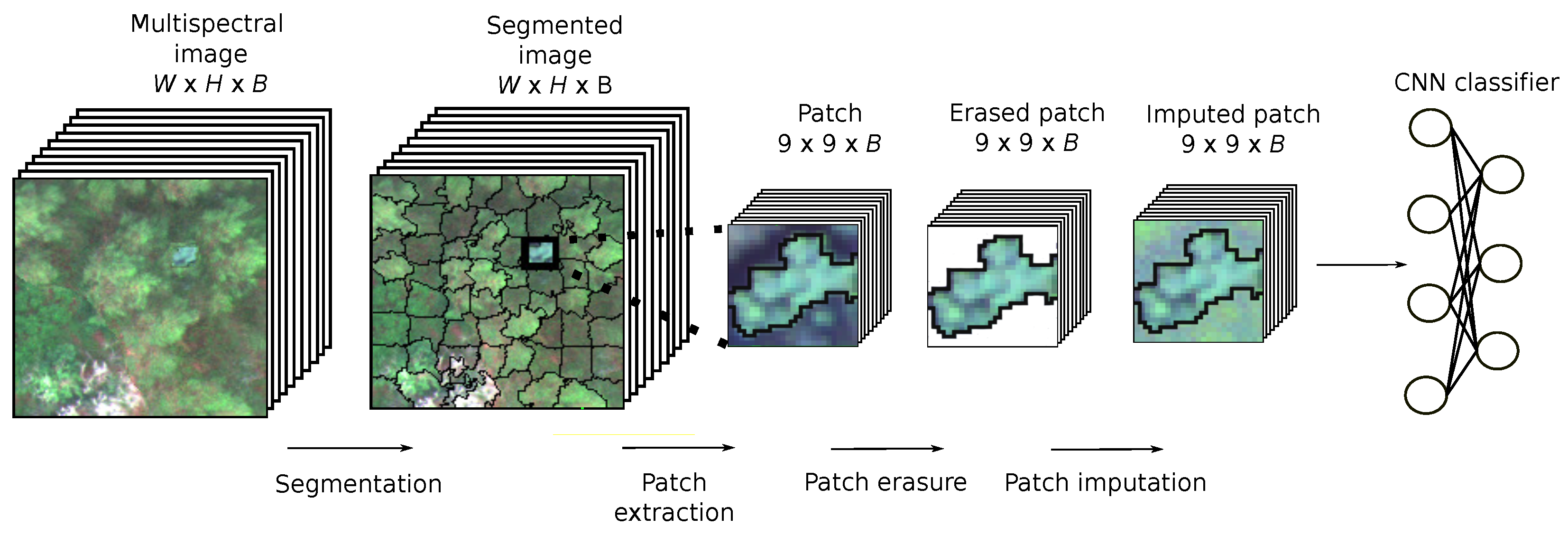
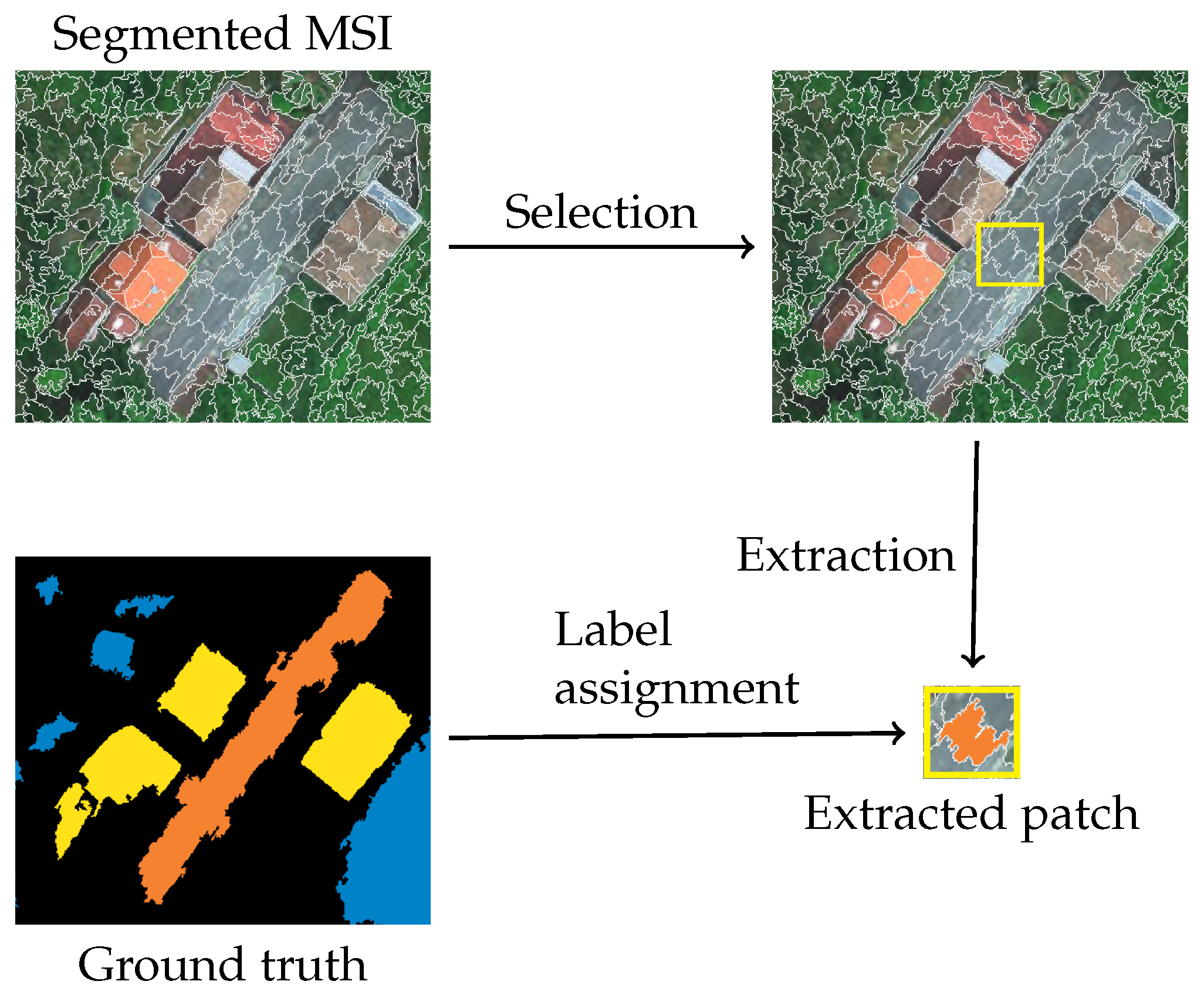
Figure 2.
Stage 2: Patch extraction.
Figure 2.
Stage 2: Patch extraction.
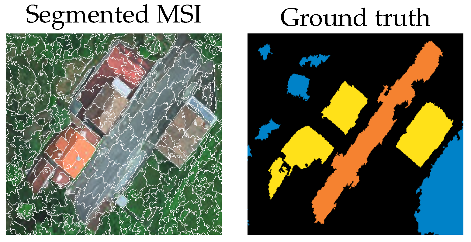
Figure 3.
Cropped section of the River Oitaven scene after superpixel segmentation along with the corresponding reference data.
Figure 3.
Cropped section of the River Oitaven scene after superpixel segmentation along with the corresponding reference data.
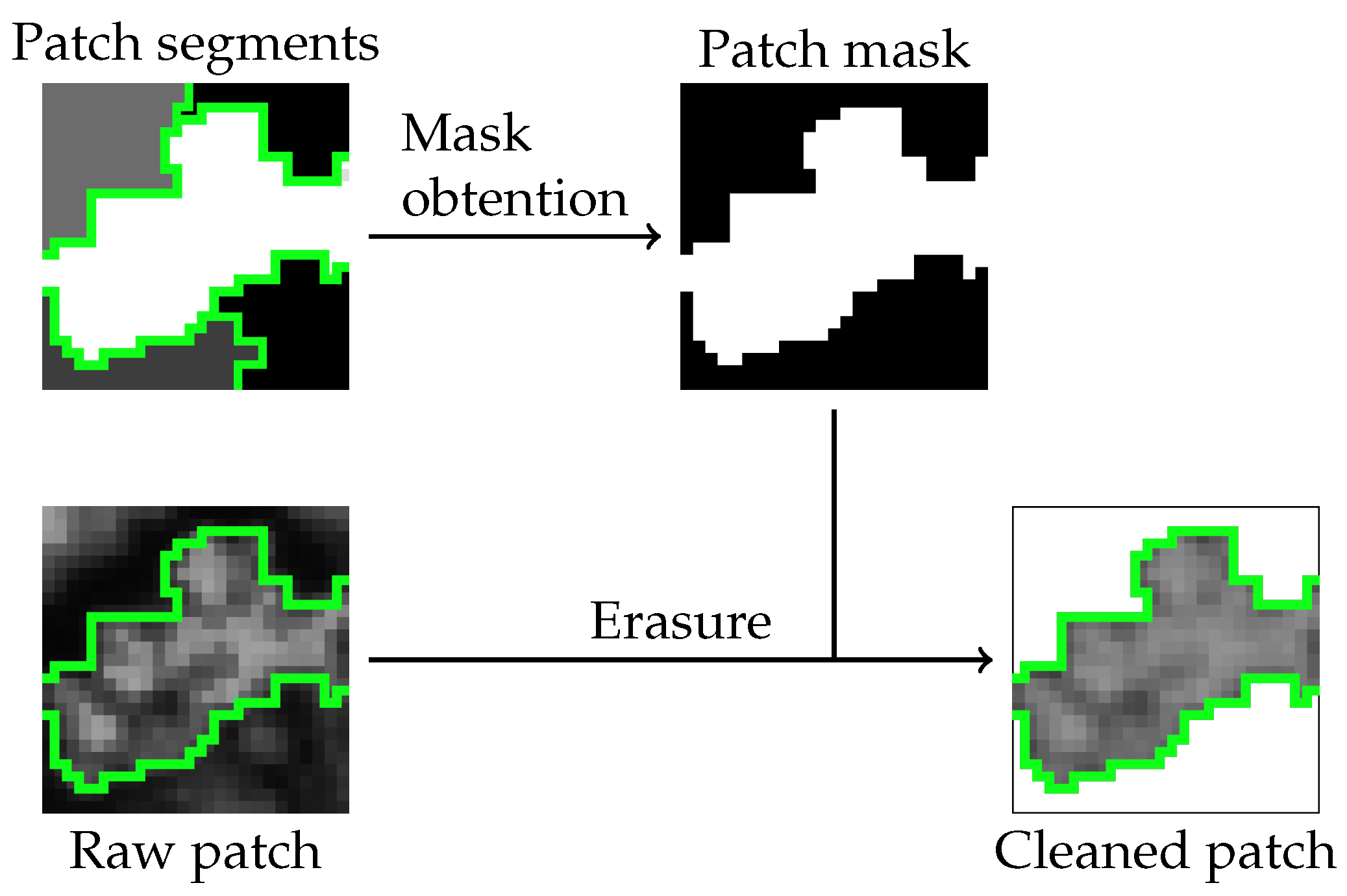
Figure 4.
Stage 3: Patch erasure.
Figure 4.
Stage 3: Patch erasure.
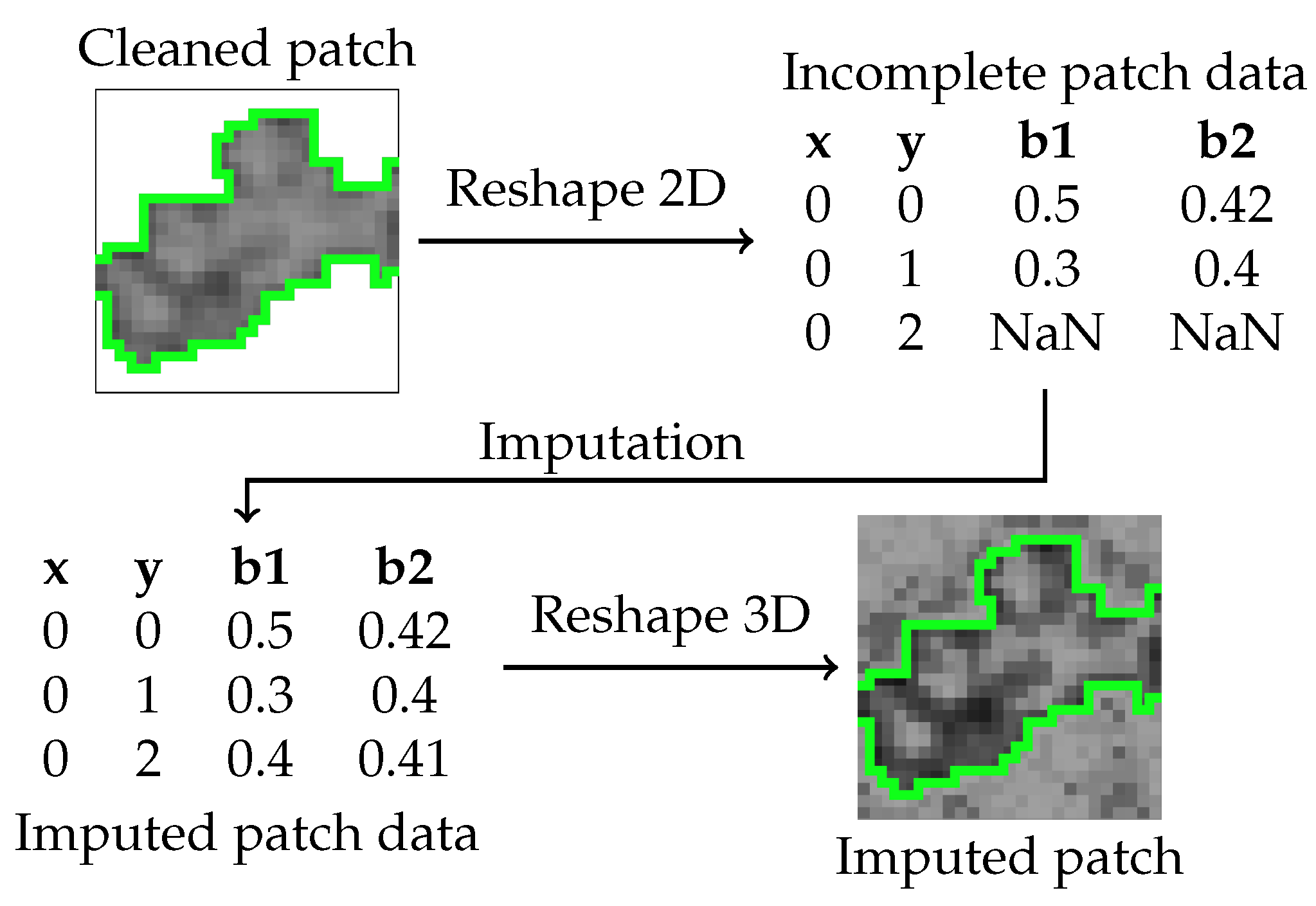
Figure 5.
Stage 4: Patch imputation.
Figure 5.
Stage 4: Patch imputation.
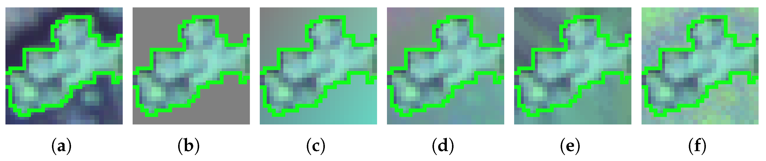
Figure 6.
Example of augmented patches for each of the studied imputation methods, for a segment of the River Mestas scene with a segment size of 800, and a patch size of . (a) None, (b) Constant, (c) SoftImpute, (d) SVDimpute, (e) KNNimpute, (f) MICE.
Figure 6.
Example of augmented patches for each of the studied imputation methods, for a segment of the River Mestas scene with a segment size of 800, and a patch size of . (a) None, (b) Constant, (c) SoftImpute, (d) SVDimpute, (e) KNNimpute, (f) MICE.
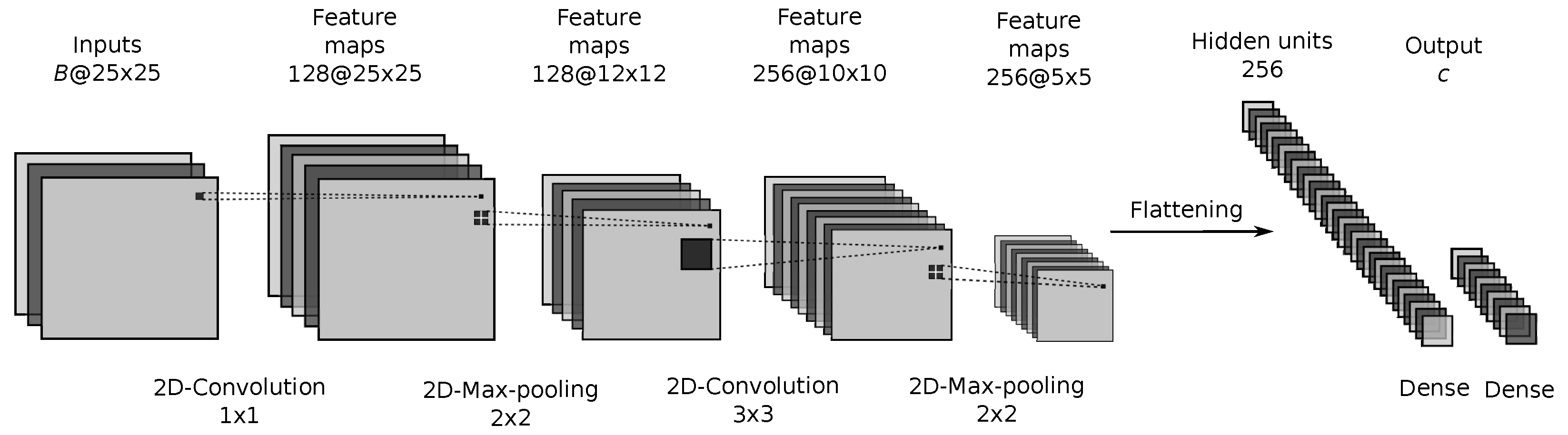
Figure 7.
Proposed CNN architecture.
Figure 7.
Proposed CNN architecture.
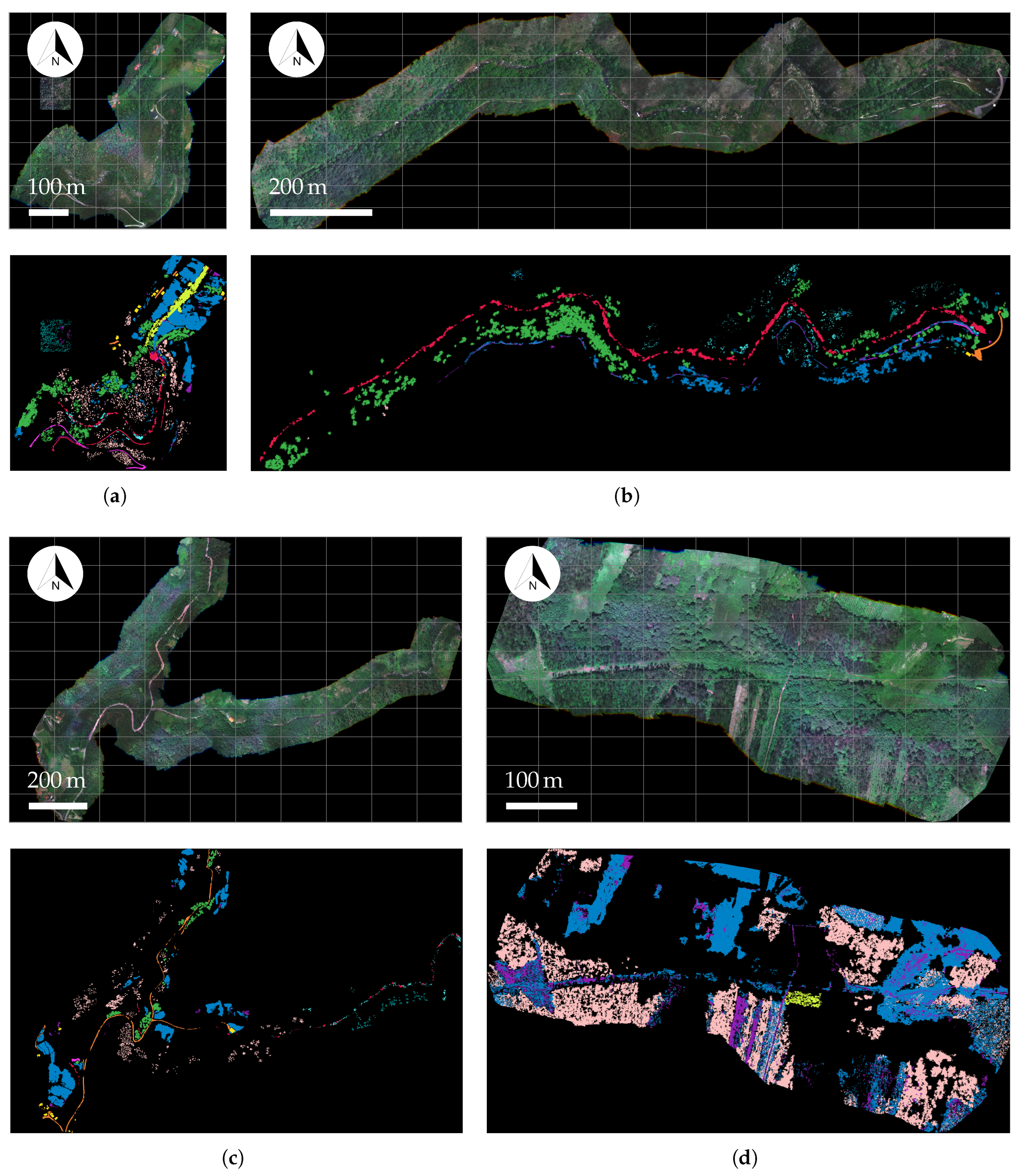
Figure 8.
False color composite and ground truth for scenes from the Galicia dataset: (
a) Oitaven, (
b) Eiras, (
c) Ermidas and (
d) Mestas. Color codes are the same as those introduced in
Table 2.
Figure 8.
False color composite and ground truth for scenes from the Galicia dataset: (
a) Oitaven, (
b) Eiras, (
c) Ermidas and (
d) Mestas. Color codes are the same as those introduced in
Table 2.
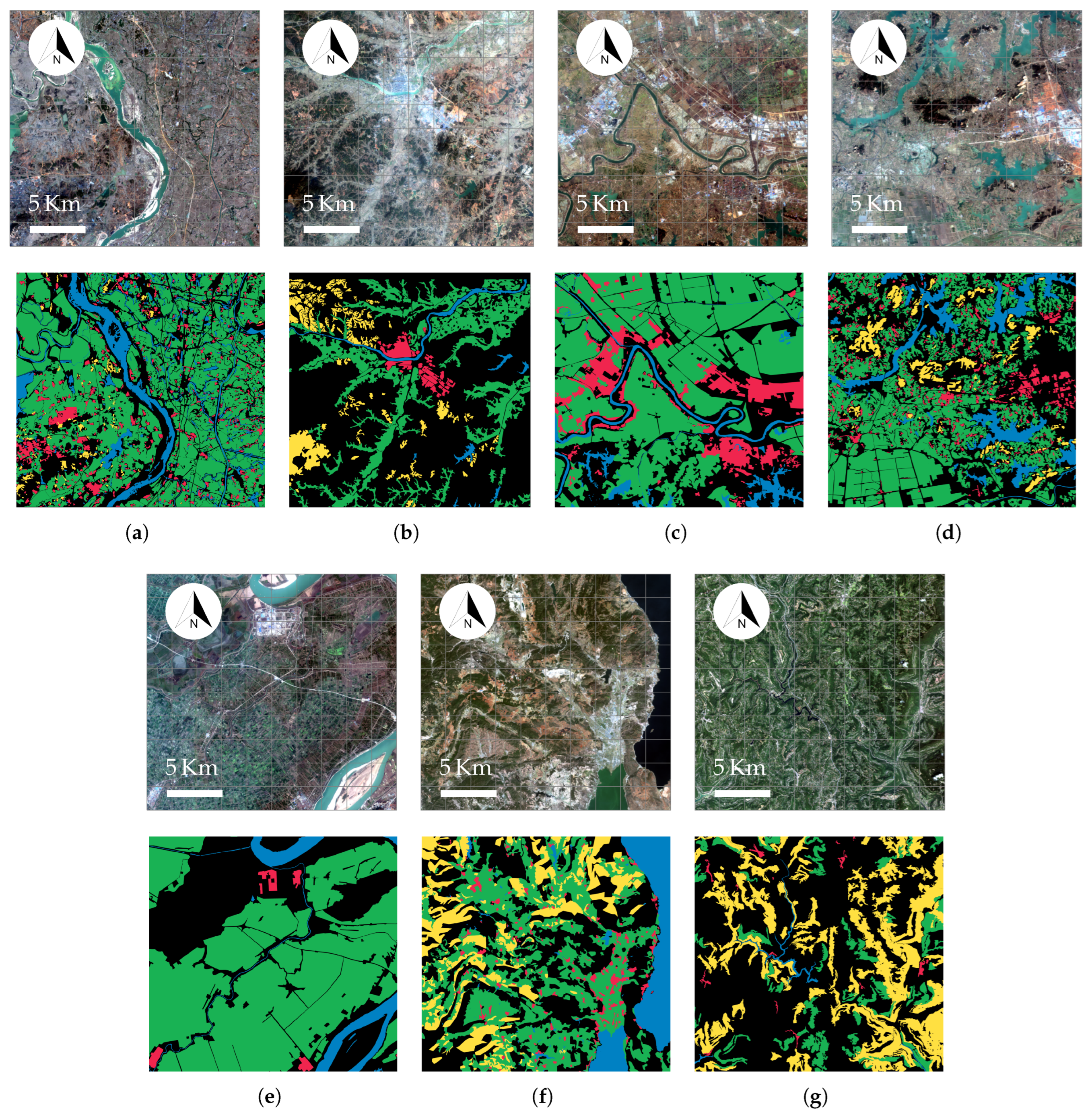
Figure 9.
False color composite and ground truth for scenes from the GID: (
a) GF2-5A, (
b) GF2-5B, (
c) GF2-5C, (
d) GF2-5D, (
e) GF2-5E, (
f) GF2-5F, and (
g) GF2-5G. Color codes are the same as those introduced in
Table 3.
Figure 9.
False color composite and ground truth for scenes from the GID: (
a) GF2-5A, (
b) GF2-5B, (
c) GF2-5C, (
d) GF2-5D, (
e) GF2-5E, (
f) GF2-5F, and (
g) GF2-5G. Color codes are the same as those introduced in
Table 3.
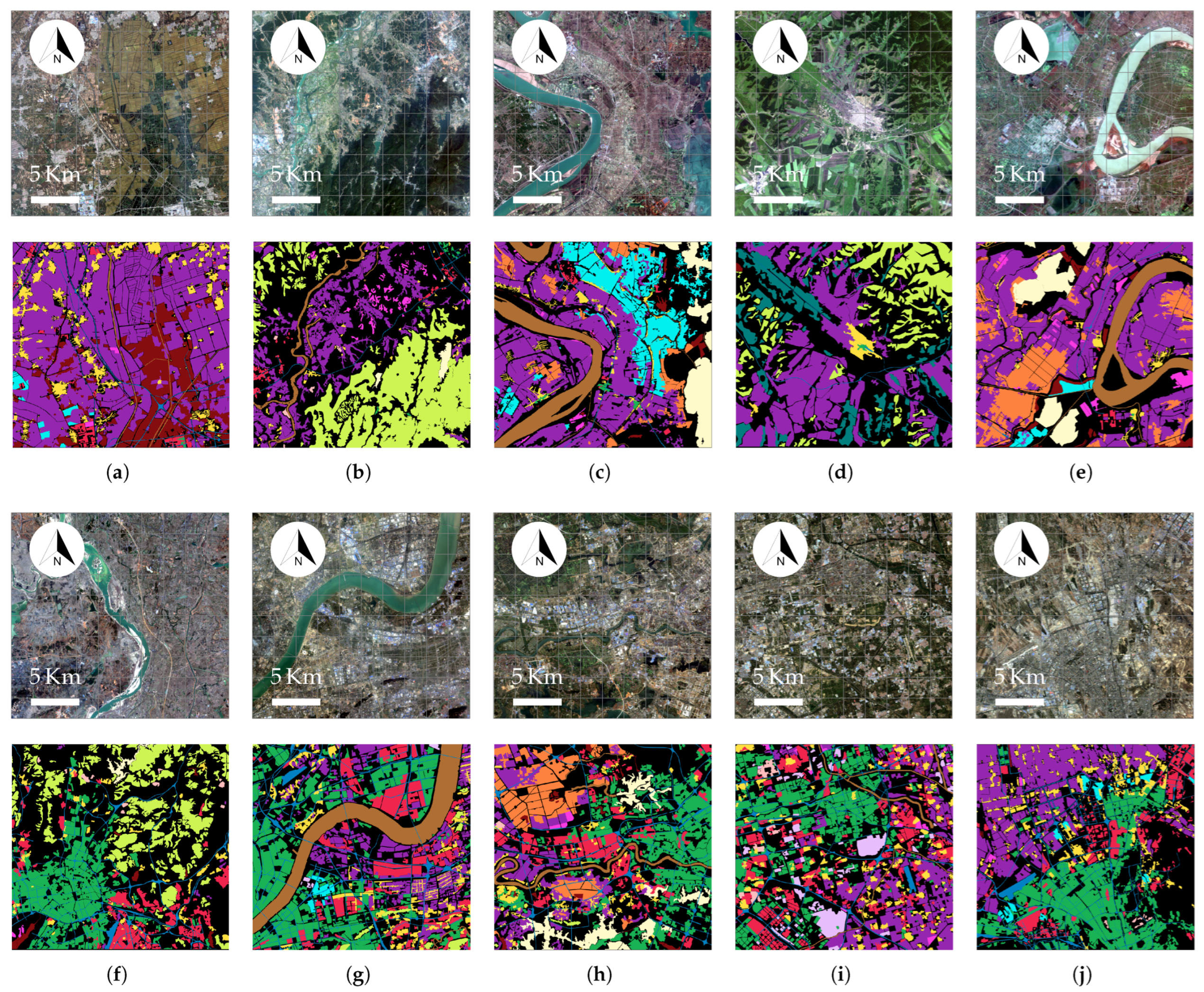
Figure 10.
False color composite and ground truth for scenes from the GID: (
a) GF2-15A, (
b) GF2-15B, (
c) GF2-15C, (
d) GF2-15D, (
e) GF2-15E, (
f) GF2-15F, (
g) GF2-15G, (
h) GF2-15H, (
i) GF2-15I, and (
j) GF2-15J. Color codes are the same as those introduced in
Table 4.
Figure 10.
False color composite and ground truth for scenes from the GID: (
a) GF2-15A, (
b) GF2-15B, (
c) GF2-15C, (
d) GF2-15D, (
e) GF2-15E, (
f) GF2-15F, (
g) GF2-15G, (
h) GF2-15H, (
i) GF2-15I, and (
j) GF2-15J. Color codes are the same as those introduced in
Table 4.
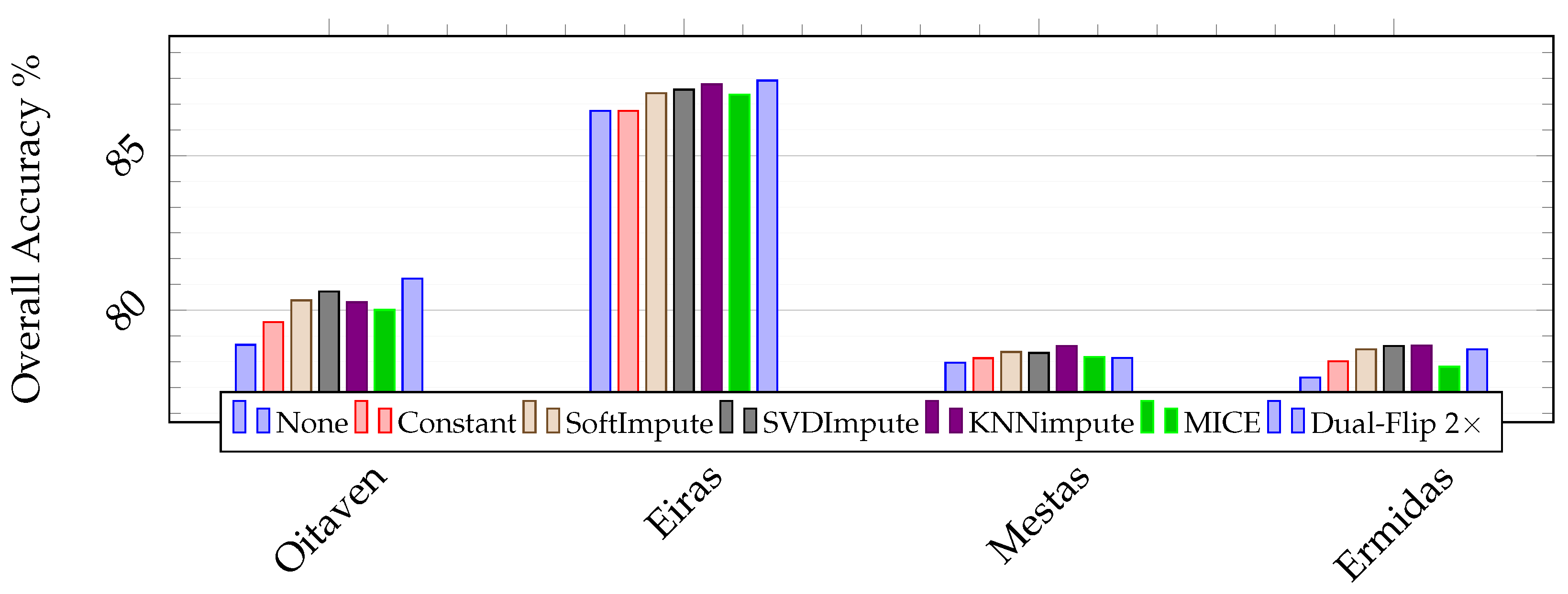
Figure 11.
Classification performance (in percent) for the scenes from the for the scenes of the Galicia dataset. None denotes the baseline, or training with no data augmentation.
Figure 11.
Classification performance (in percent) for the scenes from the for the scenes of the Galicia dataset. None denotes the baseline, or training with no data augmentation.
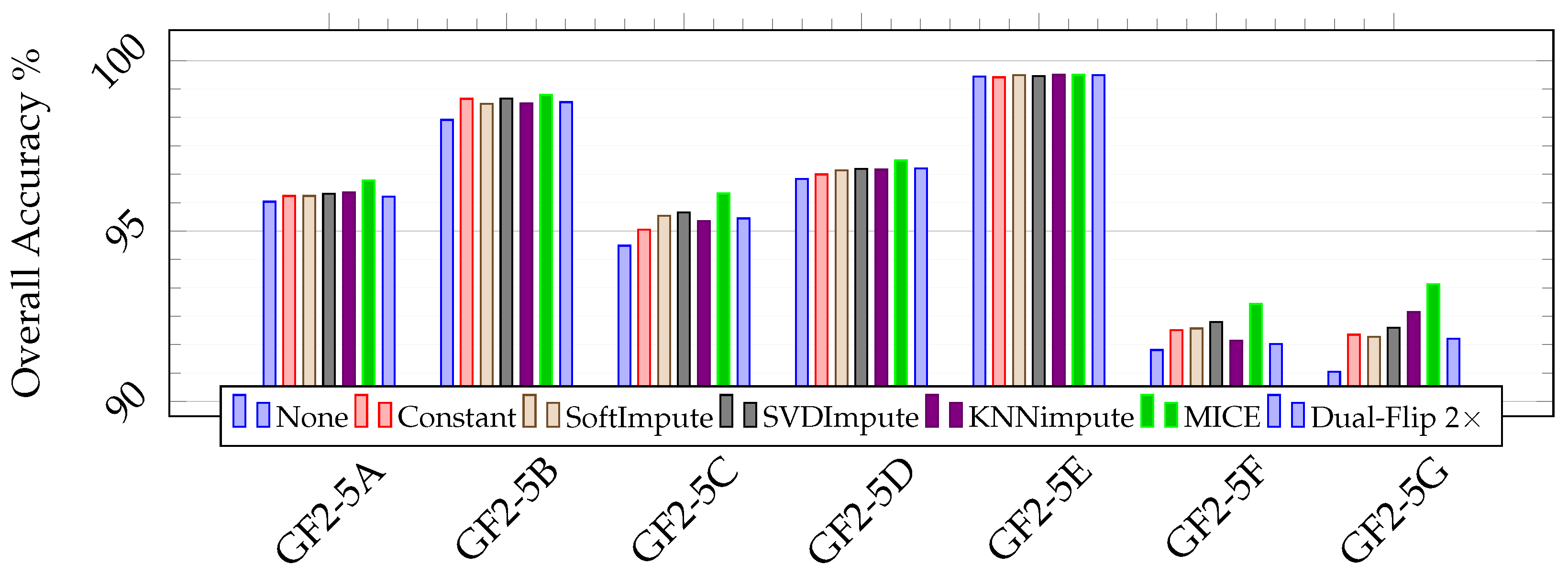
Figure 12.
Classification performance (in percent) for the scenes from the 5-class large scale classification set of the GID. None denotes the baseline, or training with no data augmentation.
Figure 12.
Classification performance (in percent) for the scenes from the 5-class large scale classification set of the GID. None denotes the baseline, or training with no data augmentation.
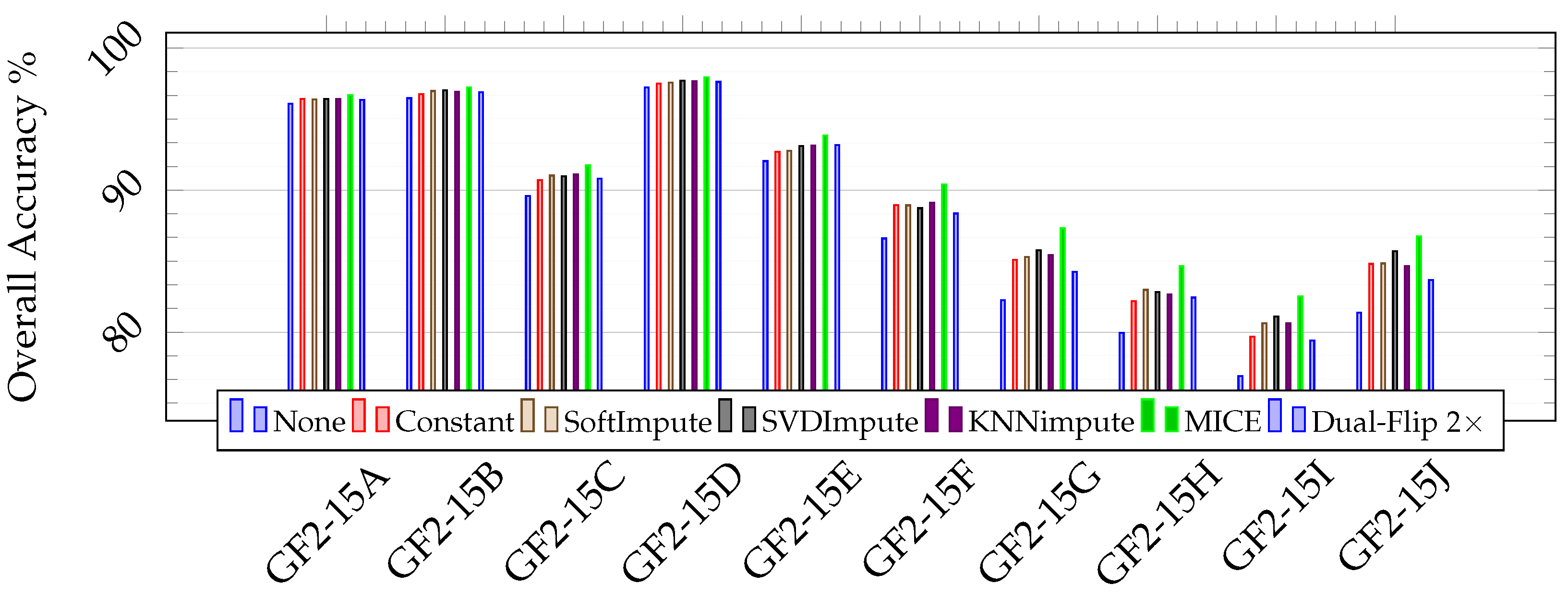
Figure 13.
Classification performance (in percent) for the scenes from the 15-class large scale classification set of the GID. None denotes the baseline, or training with no data augmentation.
Figure 13.
Classification performance (in percent) for the scenes from the 15-class large scale classification set of the GID. None denotes the baseline, or training with no data augmentation.
Table 1.
Neural network architecture.
Table 1.
Neural network architecture.
| # | Type | Output Shape | Activation | Filter Size | Stride |
|---|
| 1 | 2D-Convolutional | | ELU | | |
| 2 | 2D-MaxPooling | | - | | |
| 3 | 2D-Convolutional | | ELU | | |
| 4 | 2D-MaxPooling | | - | | |
| 5 | Dropout | | - | - | - |
| 6 | Flatten | | - | - | - |
| 7 | Dense | | ELU | - | - |
| 8 | Dropout | | - | - | - |
| 9 | Dense | | Softmax | - | - |
Table 2.
Galicia dataset. Oitaven, Ermidas, Eiras and Mestas scenes. Color codes for the classes and number of superpixels in the training and testing sets. The “-” symbol denotes the absence of samples for the specified class.
Table 2.
Galicia dataset. Oitaven, Ermidas, Eiras and Mestas scenes. Color codes for the classes and number of superpixels in the training and testing sets. The “-” symbol denotes the absence of samples for the specified class.
| | Oitaven | Ermidas |
|---|
| # | Classes | Train | Test | Classes | Train | Test |
| 1. | Water | 367 | 120 | Water | 183 | 70 |
| 2. | Oak | 2227 | 739 | Oak | 1201 | 390 |
| 3. | Tiles | 112 | 48 | Tiles | 137 | 33 |
| 4. | Meadows | 2709 | 863 | Meadows | 3550 | 1142 |
| 5. | Asphalt | 52 | 14 | Asphalt | 976 | 331 |
| 6. | Bare Soil | 256 | 92 | Bare Soil | 253 | 83 |
| 7. | Rock | 192 | 72 | Rock | 522 | 172 |
| 8. | Concrete | 206 | 79 | Concrete | 45 | 8 |
| 9. | Endemic veg. | 592 | 197 | Endemic veg. | - | - |
| 10. | Eucaliptus | 2553 | 838 | Eucaliptus | 2704 | 926 |
| 11. | Pines | 430 | 151 | Pines | 413 | 149 |
| | Eiras | Mestas |
| # | Classes | Train | Test | Classes | Train | Test |
| 1. | Water | 823 | 278 | Water | - | - |
| 2. | Oak | 3332 | 1066 | Oak | - | - |
| 3. | Tiles | 12 | 2 | Tiles | - | - |
| 4. | Meadows | 1476 | 485 | Meadows | 5373 | 1780 |
| 5. | Asphalt | 86 | 32 | Asphalt | - | - |
| 6. | Bare Soil | 247 | 86 | Bare Soil | 1653 | 487 |
| 7. | Rock | 830 | 286 | Rock | - | - |
| 8. | Concrete | 56 | 16 | Concrete | - | - |
| 9. | Endemic veg. | - | - | Endemic veg. | 138 | 40 |
| 10. | Eucaliptus | 23 | 5 | Eucaliptus | 5540 | 1887 |
| 11. | Pines | 187 | 70 | Pines | - | - |
Table 3.
Scenes from the 5-class large scene classification set of the GID. Color codes for the classes and number of superpixels in the training and testing sets. The “-” symbol denotes the absence of samples for the specified class. Classes are, in ascending order, built-up, farmland, forest, meadow, and water.
| | Classes | | Classes |
|---|
| Set | 1 | 2 | 3 | 4 | 5 | Set | 1 | 2 | 3 | 4 | 5 |
|---|
| GF2_PMS1__L1A0000564539-MSS1 - GF2-5A | GF2_PMS1__L1A0000647770-MSS1 - GF2-5E |
| Train | 3547 | 27,699 | 755 | 5151 | - | Train | 591 | 32,054 | - | 2139 | - |
| Test | 1109 | 9244 | 246 | 1737 | - | Test | 204 | 10,595 | - | 729 | - |
| GF2_PMS1__L1A0000575925-MSS1 - GF2-5B | GF2_PMS1__L1A0000708367-MSS1 - GF2-5F |
| Train | 1295 | 12,351 | 3759 | 1027 | - | Train | 1663 | 19,207 | 6795 | 4143 | - |
| Test | 477 | 4102 | 1219 | 345 | - | Test | 543 | 6382 | 2237 | 1395 | - |
| GF2_PMS1__L1A0000647767-MSS1 - GF2-5C | GF2_PMS1__L1A0000962382-MSS1 - GF2-5G |
| Train | 6432 | 27,704 | - | 2920 | - | Train | 476 | 5225 | 12,942 | 397 | - |
| Test | 2153 | 9281 | - | 911 | - | Test | 170 | 1738 | 4279 | 119 | - |
| GF2_PMS1__L1A0000647768-MSS1 - GF2-5D | |
| Train | 3482 | 21,976 | 2316 | 3682 | - | |
| Test | 1247 | 7224 | 799 | 1204 | - | |
Table 4.
Scenes from the 15-class large scene classification set of the GID. Color codes for the classes and number of superpixels in the training and testing sets. The “-” symbol denotes the absence of samples for the specified class. Classes are, in ascending order, industrial land, urban residential, rural residential, traffic land, paddy field, irrigated land, dry cropland, garden plot, arbor woodland, shrub land, natural grassland, artificial grassland, river, lake, and pond.
| | Classes |
|---|
| Set | 1 | 2 | 3 | 4 | 5 | 6 | 7 | 8 | 9 | 10 | 11 | 12 | 13 | 14 | 15 |
|---|
| GF2_PMS1__L1A0001064454-MSS1 - GF2-15A |
| Train | 1001 | 24 | 3627 | 1302 | - | 29,047 | 491 | 65 | - | - | - | - | 658 | - | 8169 |
| Test | 294 | 8 | 1238 | 442 | - | 9630 | 168 | 30 | - | - | - | - | 206 | - | 2754 |
| GF2_PMS1__L1A0001118839-MSS1 - GF2-15B |
| Train | 632 | 165 | 564 | 774 | - | 9009 | - | 871 | 13,310 | 126 | - | - | 968 | 291 | 10 |
| Test | 191 | 49 | 182 | 272 | - | 2958 | - | 296 | 4440 | 45 | - | - | 337 | 90 | 6 |
| GF2_PMS1__L1A0001395956-MSS1 - GF2-15C |
| Train | 338 | 133 | 1277 | 343 | 2596 | 17,872 | 7035 | 294 | - | - | - | - | 3728 | 2404 | 492 |
| Test | 130 | 36 | 423 | 104 | 851 | 5968 | 2296 | 89 | - | - | - | - | 1221 | 832 | 170 |
| GF2_PMS1__L1A0001680858-MSS1 - GF2-15D |
| Train | - | 28 | 565 | 714 | - | 12,686 | - | - | 5815 | - | 5122 | - | - | - | 30 |
| Test | - | 13 | 203 | 213 | - | 4225 | - | - | 1990 | - | 1634 | - | - | - | 8 |
| GF2_PMS2__L1A0000718813-MSS2 - GF2-15E |
| Train | 275 | 11 | 952 | 213 | 7462 | 20,709 | 547 | 798 | - | - | - | - | 3441 | 2608 | 872 |
| Test | 84 | 3 | 331 | 72 | 2470 | 6857 | 206 | 273 | - | - | - | - | 1164 | 856 | 277 |
| GF2_PMS2__L1A0001378501-MSS2 - GF2-15F |
| Train | 3614 | 7748 | 1102 | 3815 | - | 175 | - | 63 | 8054 | 249 | - | - | - | 290 | 330 |
| Test | 1166 | 2563 | 351 | 1229 | - | 56 | - | 24 | 2817 | 81 | - | - | - | 92 | 87 |
| GF2_PMS2__L1A0001471436-MSS2 - GF2-15G |
| Train | 6365 | 11,858 | 3001 | 5266 | - | 6557 | 382 | - | 473 | - | - | 156 | 4342 | - | - |
| Test | 2050 | 4019 | 1006 | 1788 | - | 2205 | 110 | - | 157 | - | - | 40 | 1395 | - | - |
| GF2_PMS2__L1A0001517494-MSS2 - GF2-15H |
| Train | 4727 | 9354 | 1621 | 3983 | 5383 | 4931 | - | 107 | 115 | 44 | - | - | 1061 | 2459 | 423 |
| Test | 1554 | 3094 | 599 | 1281 | 1824 | 1644 | - | 40 | 32 | 18 | - | - | 371 | 784 | 132 |
| GF2_PMS2__L1A0001787564-MSS2 - GF2-15I |
| Train | 7427 | 10,006 | 3054 | 3436 | - | 7511 | - | 307 | - | 448 | - | 2588 | 743 | - | - |
| Test | 2432 | 3362 | 1072 | 1131 | - | 2438 | - | 97 | - | 162 | - | 882 | 244 | - | - |
| GF2_PMS2__L1A0001821754-MSS2 - GF2-15A |
| Train | 4401 | 9498 | 3585 | 5299 | - | 11,754 | 711 | 92 | - | 122 | - | - | - | - | 58 |
| Test | 1519 | 3138 | 1182 | 1780 | - | 3899 | 237 | 25 | - | 29 | - | - | - | - | 28 |
Table 5.
Classification performance (in percent) for the scenes of the Galicia dataset. None denotes the baseline, or training with no data augmentation. Bold font indicates the best result for a scene.
Table 5.
Classification performance (in percent) for the scenes of the Galicia dataset. None denotes the baseline, or training with no data augmentation. Bold font indicates the best result for a scene.
| | | Oitaven | Eiras | Mestas | Ermidas |
|---|
| None | OA | 78.88 ± 0.35 | 86.45 ± 0.20 | 78.30 ± 0.29 | 77.82 ± 0.57 |
| AA | 71.93 ± 1.01 | 80.25 ± 1.70 | 71.36 ± 1.02 | 70.61 ± 0.81 |
| K | 72.92 ± 0.55 | 81.26 ± 0.26 | 66.24 ± 0.45 | 68.96 ± 0.92 |
| Constant | OA | 79.62 ± 0.46 | 86.83 ± 0.13 | 78.45 ± 0.15 | 78.35 ± 0.16 |
| AA | 73.39 ± 0.66 | 82.14 ± 0.40 | 70.63 ± 1.79 | 70.57 ± 1.28 |
| K | 73.89 ± 0.64 | 81.81 ± 0.15 | 66.52 ± 0.24 | 69.72 ± 0.28 |
| SoftImpute | OA | 80.32 ± 0.17 | 87.02 ± 0.26 | 78.65 ± 0.05 | 78.73 ± 0.26 |
| AA | 75.40 ± 0.81 | 82.05 ± 0.41 | 71.47 ± 1.68 | 72.62 ± 1.48 |
| K | 74.84 ± 0.22 | 82.02 ± 0.39 | 66.85 ± 0.09 | 70.46 ± 0.48 |
| SVDimpute | OA | 80.61 ± 0.27 | 87.14 ± 0.28 | 78.62 ± 0.08 | 78.84 ± 0.22 |
| AA | 75.56 ± 0.63 | 82.46 ± 0.49 | 71.46 ± 1.79 | 73.29 ± 1.43 |
| K | 75.22 ± 0.33 | 82.24 ± 0.40 | 66.78 ± 0.14 | 70.47 ± 0.37 |
| KNNimpute | OA | 80.26 ± 0.24 | 87.31 ± 0.23 | 78.84 ± 0.03 | 78.86 ± 0.09 |
| AA | 75.08 ± 0.80 | 82.90 ± 0.51 | 72.20 ± 0.74 | 72.52 ± 1.07 |
| K | 74.75 ± 0.33 | 82.45 ± 0.31 | 67.10 ± 0.08 | 70.48 ± 0.15 |
| MICE | OA | 80.01 ± 0.28 | 86.98 ± 0.05 | 78.49 ± 0.09 | 78.17 ± 0.28 |
| AA | 74.97 ± 0.62 | 80.95 ± 1.14 | 72.02 ± 0.75 | 69.89 ± 1.17 |
| K | 74.44 ± 0.40 | 82.00 ± 0.10 | 66.63 ± 0.10 | 69.57 ± 0.54 |
| Dual-Flip 2× [59] | OA | 81.02 ± 0.18 | 87.43 ± 0.06 | 78.46 ± 0.21 | 78.73 ± 0.18 |
| AA | 75.61 ± 0.50 | 82.77 ± 0.43 | 71.49 ± 1.10 | 73.30 ± 1.57 |
| K | 75.73 ± 0.23 | 82.60 ± 0.08 | 66.54 ± 0.34 | 70.44 ± 0.18 |
Table 6.
Classification performance (in percent) for the scenes from the 5-class large scene classification set of the GID. None denotes the baseline, or training with no data augmentation. Bold font indicates the best result for a scene.
Table 6.
Classification performance (in percent) for the scenes from the 5-class large scene classification set of the GID. None denotes the baseline, or training with no data augmentation. Bold font indicates the best result for a scene.
| | | GF2-5A | GF2-5B | GF2-5C | GF2-5D | GF2-5E | GF2-5F | GF2-5G |
|---|
| None | OA | 95.86 ± 0.04 | 98.26 ± 0.34 | 94.57 ± 0.13 | 96.53 ± 0.04 | 99.53 ± 0.05 | 91.51 ± 0.23 | 90.87 ± 0.69 |
| AA | 90.84 ± 0.66 | 95.00 ± 1.38 | 89.11 ± 0.37 | 92.69 ± 0.24 | 97.80 ± 0.35 | 85.37 ± 0.53 | 80.96 ± 2.57 |
| K | 89.38 ± 0.10 | 96.40 ± 0.73 | 85.81 ± 0.37 | 92.83 ± 0.09 | 97.20 ± 0.26 | 86.21 ± 0.41 | 77.61 ± 2.07 |
| Constant | OA | 96.03 ± 0.06 | 98.88 ± 0.09 | 95.04 ± 0.46 | 96.66 ± 0.29 | 99.51 ± 0.04 | 92.09 ± 0.19 | 91.96 ± 0.42 |
| AA | 91.33 ± 0.46 | 97.44 ± 0.38 | 90.25 ± 2.21 | 93.37 ± 1.19 | 97.90 ± 0.40 | 86.13 ± 0.67 | 84.03 ± 3.00 |
| K | 89.80 ± 0.17 | 97.71 ± 0.18 | 87.19 ± 1.31 | 93.12 ± 0.64 | 97.08 ± 0.22 | 87.12 ± 0.33 | 80.46 ± 1.28 |
| SoftImpute | OA | 96.03 ± 0.16 | 98.73 ± 0.15 | 95.45 ± 0.11 | 96.78 ± 0.10 | 99.57 ± 0.03 | 92.14 ± 0.31 | 91.90 ± 0.29 |
| AA | 90.44 ± 1.74 | 96.73 ± 0.80 | 91.84 ± 0.51 | 93.80 ± 0.36 | 97.80 ± 0.18 | 86.74 ± 1.27 | 85.87 ± 0.92 |
| K | 89.80 ± 0.47 | 97.39 ± 0.31 | 88.39 ± 0.28 | 93.39 ± 0.20 | 97.47 ± 0.19 | 87.27 ± 0.58 | 80.17 ± 0.80 |
| SVDImpute | OA | 96.09 ± 0.06 | 98.89 ± 0.06 | 95.55 ± 0.05 | 96.82 ± 0.08 | 99.55 ± 0.03 | 92.33 ± 0.08 | 92.16 ± 0.40 |
| AA | 91.42 ± 0.67 | 97.35 ± 0.30 | 91.18 ± 0.44 | 93.73 ± 0.45 | 97.77 ± 0.70 | 87.05 ± 0.48 | 86.69 ± 0.89 |
| K | 90.00 ± 0.16 | 97.73 ± 0.12 | 88.54 ± 0.14 | 93.46 ± 0.20 | 97.31 ± 0.19 | 87.53 ± 0.13 | 80.87 ± 1.13 |
| KNNimpute | OA | 96.13 ± 0.10 | 98.75 ± 0.22 | 95.29 ± 0.31 | 96.80 ± 0.05 | 99.59 ± 0.04 | 91.78 ± 0.51 | 92.62 ± 0.19 |
| AA | 91.51 ± 0.43 | 97.47 ± 0.24 | 90.88 ± 0.52 | 93.82 ± 0.47 | 97.62 ± 0.55 | 86.47 ± 0.83 | 87.14 ± 0.23 |
| K | 90.10 ± 0.24 | 97.45 ± 0.44 | 87.83 ± 0.84 | 93.43 ± 0.12 | 97.57 ± 0.23 | 86.58 ± 0.90 | 82.07 ± 0.56 |
| MICE | OA | 96.49 ± 0.05 | 98.99 ± 0.21 | 96.10 ± 0.08 | 97.07 ± 0.07 | 99.58 ± 0.06 | 92.86 ± 0.10 | 93.44 ± 0.24 |
| AA | 91.96 ± 0.32 | 97.86 ± 0.30 | 93.34 ± 0.51 | 93.92 ± 0.30 | 97.36 ± 0.84 | 88.07 ± 0.40 | 88.39 ± 0.75 |
| K | 91.03 ± 0.14 | 97.93 ± 0.42 | 90.08 ± 0.15 | 93.96 ± 0.16 | 97.51 ± 0.37 | 88.45 ± 0.18 | 84.24 ± 0.67 |
| Dual-Flip 2× [59] | OA | 96.01 ± 0.06 | 98.78 ± 0.17 | 95.37 ± 0.18 | 96.84 ± 0.08 | 99.57 ± 0.07 | 91.69 ± 0.36 | 91.84 ± 0.39 |
| AA | 91.30 ± 0.38 | 97.07 ± 0.28 | 91.52 ± 0.91 | 93.59 ± 0.41 | 97.44 ± 0.89 | 85.60 ± 0.85 | 84.82 ± 0.90 |
| K | 89.72 ± 0.19 | 97.50 ± 0.35 | 88.12 ± 0.44 | 93.49 ± 0.18 | 97.43 ± 0.42 | 86.46 ± 0.65 | 80.08 ± 1.13 |
Table 7.
Classification performance (in percent) for the scenes from the 15-class large scale classification set of the GID. None denotes the baseline, or training with no data augmentation. Bold font indicates the best result for a scene.
Table 7.
Classification performance (in percent) for the scenes from the 15-class large scale classification set of the GID. None denotes the baseline, or training with no data augmentation. Bold font indicates the best result for a scene.
| | | GF2-15A | GF2-15B | GF2-15C | GF2-15D | GF2-15E | GF2-15F | GF2-15G | GF2-15H | GF2-15I | GF2-15J |
|---|
| None | OA | 96.08 ± 0.05 | 96.47 ± 0.11 | 89.58 ± 0.11 | 97.24 ± 0.15 | 92.04 ± 0.16 | 86.6 ± 0.20 | 82.25 ± 0.13 | 79.96 ± 0.23 | 76.91 ± 0.41 | 81.38 ± 0.18 |
| AA | 73.07 ± 0.36 | 74.42 ± 1.59 | 76.38 ± 1.57 | 87.98 ± 1.19 | 75.24 ± 1.89 | 75.00 ± 0.71 | 78.91 ± 1.05 | 60.49 ± 1.18 | 66.06 ± 1.87 | 68.11 ± 2.00 |
| K | 92.24 ± 0.10 | 93.97 ± 0.21 | 85.69 ± 0.13 | 95.59 ± 0.25 | 87.94 ± 0.28 | 81.75 ± 0.22 | 78.07 ± 0.19 | 76.00 ± 0.28 | 71.31 ± 0.55 | 75.08 ± 0.27 |
| Constant | OA | 96.41 ± 0.06 | 96.76 ± 0.19 | 90.71 ± 0.20 | 97.5 ± 0.08 | 92.69 ± 0.22 | 88.95 ± 0.12 | 85.08 ± 0.37 | 82.18 ± 0.29 | 79.69 ± 0.45 | 84.8 ± 0.22 |
| AA | 79.49 ± 0.67 | 74.54 ± 1.19 | 77.80 ± 1.82 | 87.22 ± 5.79 | 79.27 ± 0.74 | 78.98 ± 1.28 | 80.67 ± 1.56 | 66.94 ± 1.27 | 69.75 ± 2.62 | 70.3 ± 2.10 |
| K | 92.93 ± 0.11 | 94.48 ± 0.32 | 87.25 ± 0.31 | 96.03 ± 0.12 | 88.99 ± 0.33 | 84.97 ± 0.18 | 81.52 ± 0.47 | 78.62 ± 0.33 | 74.78 ± 0.58 | 79.62 ± 0.27 |
| SoftImpute | OA | 96.38 ± 0.07 | 97.03 ± 0.20 | 90.98 ± 0.18 | 97.56 ± 0.16 | 92.77 ± 0.23 | 88.93 ± 0.22 | 85.29 ± 0.17 | 82.98 ± 0.11 | 80.63 ± 0.31 | 84.84 ± 0.28 |
| AA | 78.65 ± 1.14 | 80.83 ± 3.17 | 79.29 ± 0.97 | 89.56 ± 0.68 | 77.64 ± 1.18 | 78.76 ± 1.42 | 81.75 ± 1.18 | 69.71 ± 1.43 | 70.99 ± 2.10 | 70.75 ± 2.01 |
| K | 92.87 ± 0.13 | 94.93 ± 0.35 | 87.63 ± 0.28 | 96.10 ± 0.27 | 89.07 ± 0.38 | 84.89 ± 0.31 | 81.8 ± 0.19 | 79.59 ± 0.16 | 75.87 ± 0.43 | 79.72 ± 0.36 |
| SVDImpute | OA | 96.43 ± 0.12 | 96.98 ± 0.34 | 91.03 ± 0.12 | 97.70 ± 0.08 | 93.10 ± 0.04 | 88.73 ± 0.24 | 85.77 ± 0.19 | 82.82 ± 0.60 | 81.11 ± 0.47 | 85.70 ± 0.26 |
| AA | 80.14 ± 2.94 | 81.24 ± 3.62 | 79.50 ± 0.50 | 88.90 ± 1.17 | 78.95 ± 0.41 | 79.00 ± 0.97 | 82.88 ± 0.57 | 66.81 ± 3.14 | 71.15 ± 1.90 | 72.75 ± 1.62 |
| K | 92.97 ± 0.23 | 94.86 ± 0.60 | 87.71 ± 0.15 | 96.33 ± 0.12 | 89.64 ± 0.09 | 84.60 ± 0.37 | 82.37 ± 0.23 | 79.37 ± 0.78 | 76.48 ± 0.67 | 80.82 ± 0.34 |
| KNNimpute | OA | 96.41 ± 0.07 | 96.93 ± 0.33 | 91.09 ± 0.20 | 97.66 ± 0.16 | 93.15 ± 0.12 | 89.11 ± 0.21 | 85.41 ± 0.15 | 82.64 ± 0.24 | 80.63 ± 0.28 | 84.66 ± 0.42 |
| AA | 79.14 ± 0.84 | 78.02 ± 2.04 | 78.84 ± 2.22 | 89.30 ± 0.41 | 79.17 ± 0.79 | 79.67 ± 1.56 | 81.75 ± 0.42 | 69.27 ± 1.90 | 71.24 ± 0.77 | 70.93 ± 2.20 |
| K | 92.93 ± 0.15 | 94.78 ± 0.53 | 87.79 ± 0.30 | 96.27 ± 0.27 | 89.7 ± 0.18 | 85.14 ± 0.32 | 81.93 ± 0.22 | 79.18 ± 0.31 | 75.91 ± 0.34 | 79.38 ± 0.62 |
| MICE | OA | 96.68 ± 0.05 | 97.23 ± 0.32 | 91.73 ± 0.36 | 97.93 ± 0.07 | 93.86 ± 0.11 | 90.39 ± 0.28 | 87.31 ± 0.18 | 84.63 ± 0.28 | 82.52 ± 0.18 | 86.74 ± 0.22 |
| AA | 78.32 ± 1.76 | 82.21 ± 2.34 | 80.22 ± 1.76 | 87.33 ± 0.43 | 80.37 ± 0.95 | 82.28 ± 2.51 | 84.62 ± 0.47 | 72.92 ± 1.11 | 73.78 ± 0.89 | 73.58 ± 1.55 |
| K | 93.46 ± 0.10 | 95.28 ± 0.55 | 88.68 ± 0.48 | 96.69 ± 0.12 | 90.76 ± 0.15 | 86.94 ± 0.37 | 84.31 ± 0.23 | 81.59 ± 0.35 | 78.25 ± 0.22 | 82.24 ± 0.29 |
| Dual-Flip 2× [59] | OA | 96.36 ± 0.06 | 96.90 ± 0.12 | 90.81 ± 0.07 | 97.62 ± 0.08 | 93.17 ± 0.19 | 88.35 ± 0.10 | 84.25 ± 0.22 | 82.44 ± 0.08 | 79.41 ± 0.41 | 83.68 ± 0.10 |
| AA | 78.69 ± 0.78 | 80.47 ± 3.96 | 77.73 ± 1.03 | 86.39 ± 0.87 | 76.76 ± 1.81 | 77.90 ± 0.96 | 80.59 ± 0.94 | 66.71 ± 0.95 | 68.64 ± 1.42 | 68.80 ± 2.70 |
| K | 92.83 ± 0.12 | 94.72 ± 0.21 | 87.38 ± 0.12 | 96.20 ± 0.12 | 89.69 ± 0.31 | 84.15 ± 0.17 | 80.52 ± 0.27 | 78.95 ± 0.10 | 74.37 ± 0.55 | 78.08 ± 0.19 |
Table 8.
Execution times (in seconds) for the scenes from the 15-class large scale classification set of the GID. None denotes the baseline, or training with no data augmentation. Bold font indicates the best result for a scene.
Table 8.
Execution times (in seconds) for the scenes from the 15-class large scale classification set of the GID. None denotes the baseline, or training with no data augmentation. Bold font indicates the best result for a scene.
| | | GF2-15A | GF2-15B | GF2-15C | GF2-15D | GF2-15E | GF2-15F | GF2-15G | GF2-15H | GF2-15I | GF2-15J |
|---|
| None | Train | 769.7 | 472.3 | 644.0 | 439.5 | 641.6 | 450.8 | 681.2 | 612.1 | 640.2 | 638.0 |
| Pred. | 35.7 | 33.8 | 35.8 | 29.8 | 35.3 | 33.6 | 36.1 | 35.9 | 35.7 | 35.1 |
| Constant | Train | 1267.8 | 769.9 | 1051.3 | 723.8 | 1084.3 | 639.2 | 1174.7 | 948.9 | 874.2 | 974.2 |
| Pred. | 48.8 | 45.5 | 49.4 | 41.5 | 44.3 | 48.3 | 48.9 | 50.9 | 50.7 | 49.9 |
| SoftImpute | Train | 1829.9 | 1120.6 | 1530.2 | 1052.2 | 1577.1 | 1080.2 | 1616.2 | 1445.5 | 1501.6 | 1501.6 |
| Pred. | 45.7 | 41.9 | 45.5 | 38.5 | 44.4 | 42.7 | 46.2 | 46.0 | 45.2 | 45.4 |
| SVDImpute | Train | 1763.1 | 1231.6 | 1697.6 | 1161.0 | 1741.1 | 1231.3 | 1828.6 | 1659.6 | 1779.9 | 1758.2 |
| Pred. | 45.3 | 42.2 | 45.3 | 38.4 | 44.3 | 42.5 | 46.0 | 45.8 | 45.6 | 45.4 |
| KNNimpute | Train | 3625.8 | 2379.2 | 3049.1 | 2181.3 | 3152 | 2250.8 | 3346.7 | 2920.0 | 3087.0 | 3040.0 |
| Pred. | 45.6 | 42.1 | 45.4 | 38.5 | 44.2 | 42.7 | 46.2 | 45.8 | 45.1 | 45.2 |
| MICE | Train | 1848.4 | 1126.2 | 1436.2 | 985.8 | 1495.7 | 1603.3 | 2051.1 | 2070.4 | 2994.7 | 2361.8 |
| Pred. | 45.3 | 42.5 | 45.5 | 38.5 | 44.3 | 42.8 | 46.1 | 4 | 45.42 | 45.46 |
| Dual-Flip 2× [59] | Train | 1081.5 | 674.3 | 922.0 | 623.40 | 960.6 | 635.3 | 976.1 | 733.7 | 857.2 | 878.6 |
| Pred. | 60.9 | 51.8 | 56.7 | 46.7 | 54.8 | 49.8 | 56.9 | 57.3 | 54.0 | 55.4 |


