Article

Impact of Climate Change on the Hydrological Regime of the Yarkant River Basin, China: An Assessment Using Three SSP Scenarios of CMIP6 GCMs

1
School of Public Administration, Shanxi University of Finance and Economics, Taiyuan 030006, China
2
State Key Laboratory of Desert and Oasis Ecology, Xinjiang Institute of Ecology and Geography, Chinese Academy of Sciences, Urumqi 830011, China
3
School of Water Resources and Hydropower Engineering, North China Electric Power University, Beijing 102206, China
4
School of Geographical Sciences, Shanxi Normal University, Taiyuan 030000, China
*
Author to whom correspondence should be addressed.
Remote Sens. 2022, 14(1), 115; https://doi.org/10.3390/rs14010115
Submission received: 19 November 2021 / Revised: 19 December 2021 / Accepted: 23 December 2021 / Published: 28 December 2021
(This article belongs to the Special Issue Remote Sensing for Climate Extremes and Water Resources)

Abstract

:
Quantification of the impacts of climate change on streamflow and other hydrological parameters is of high importance and remains a challenge in arid areas. This study applied a modified distributed hydrological model (HEC-HMS) to the Yarkant River basin, China to assess hydrological changes under future climate change scenarios. Climate change was assessed based on six CMIP6 general circulation models (GCMs), three shared socio-economic pathways (SSP126, SSP245, SSP370), and several bias correction methods, whereas hydrological regime changes were assessed over two timeframes, referred to as the near future (2021–2049) and the far future (2071–2099). Results demonstrate that the DM (distribution mapping) and LOCI (local intensity scaling) bias correction methods most closely fit the projections of temperature and precipitation, respectively. The climate projections predicted a rise in temperature of 1.72–1.79 °C under the three SSP scenarios for the near future, and 3.76–6.22 °C under the three SSPs for the far future. Precipitation increased by 10.79–12% in the near future, and by 14.82–29.07% during the far future. It is very likely that streamflow will increase during both the near future (10.62–19.2%) and far future (36.69–70.4%) under all three scenarios. The increase in direct flow will be greater than baseflow. Summer and winter streamflow will increase the most, while the increase in streamflow was projected to reach a maximum during June and July over the near future. Over the far future, runoff reached a peak in May and June. The timing of peak streamflow will change from August to July in comparison to historical records. Both high- and low-flow magnitudes during March, April, and May (MAM) as well as June, July, and August (JJA) will increase by varying degrees, whereas the frequency of low flows will decrease during both MAM and JJA. High flow frequency in JJA was projected to decrease. Overall, our results reveal that the hydrological regime of the Yarkant River is likely to change and will be characterized by larger seasonal uncertainty and more frequent extreme events due to significant warming over the two periods. These changes should be seriously considered during policy development.

1. Introduction

Observed climate change has altered the global hydrological cycle and is expected to have a considerable impact on multi-scale freshwater availability [1]. Therefore, streamflow predictions associated with a changing climate are critically needed, especially in arid areas, for strategic and effective water resources planning and management.
The Yarkant River, located in the northwestern arid region of China, is the longest tributary of the Tarim River, which is the largest inland river in China. The Yarkant River Basin Irrigation District is the fourth largest agricultural irrigation district in China and provides water resources for a population of 1.3 million [2]. The region is characterized by a typical temperate continental arid climate and is the most important region in Xinjiang in particular, and China in general, for the production of high-quality grain, cotton, and fruits [3,4]. River runoff is a major water resource in arid basins, and often supports the development of agriculture. As an important tributary of the Tarim River, the Yarkant River provides water resources for agricultural activity and ecologically important oasis ecosystems located along the lower reaches. However, because of an increase in water consumption, the Yarkant River has not discharged water into the Tarim River since 1986. Consequently, it no longer serves as a surface water source for the Tarim River [5].
Hydrologic cycle of a basin is a complex process, which is affected by local climate, topography, soil, vegetation conditions and human activities [6]. Currently, due to the impact of global warming, glacier and snow ablation in the basin accelerates, runoff in the downstream replenishment increases, and hydrological events, such as floods and droughts, occur. These changes have a huge impact on the regional water cycle [7,8,9]. Global warming speeds up the process of water circulation and for those snow and glacier melt dominated basins, glacier and snow melt discharge increase at the same time, resulting in increased runoff downstream supplies [10]. However, for ice and snow meltwater accounting for the proportion of annual runoff in terms of small watershed, the glacier and snow “solid reservoir” reserves is limited. As a result, under the background of climate warming, the downstream river runoff is limited by its recharge, and is largely influenced by precipitation and evapotranspiration, resulting in enhanced runoff volatility [11,12]. Glacier and snow-melt water account for more than 70% of the total runoff in the Yarkant River basin. Glaciers in the Yarkant basin play a significant role in the basin’s hydrological system and are particularly sensitive to temperature changes [6]. With continuing climate change, increasing water management challenges are anticipated for the Yarkant River basin [13], and projections of future changes in temperature and water availability are of key significance.
Recently, efforts have been made to evaluate and project the impact of climate change on the hydrologic regime of the Yarkant River basin. These studies have focused on (1) the relationships between meteorological variables and streamflow using historical measurements [5,14,15]; (2) the estimation of potential changes in glacier area, mass balance, and runoff in the Yarkant River basin for the period of 2011–2050 on the basis of 17 General GCMs [16]; and (3) the estimation of changes in future glacial runoff of all rivers originating from the Tien Shan–Pamir–North Karakoram region, including the Yarkant River on the basis of hydrological and CMIP5 models. These studies found that the climatic impacts on the hydrological regime of the different watersheds are quite variable [17]. However, because of a lack of observational data, analyses have rarely analyzed the specific changes in runoff, nor have they addressed the implications of climate change on the hydrological cycle and specific hydrological components (e.g., direct runoff and baseflow) of a basin in detail. Moreover, there is a lack of prediction and analysis of the complete hydrological system in the Yarkant River under the latest climate change scenarios. This paper complements these earlier studies, which are aimed at understanding the future hydrological system of the Yarkant River basin and assesses the response of the hydrologic system to the latest climate change scenarios.
Streamflow simulations and projections represent a fundamental approach to the assessment of future water resources as needed for strategic planning and management [18]. Moreover, hydrological models serve as an important tool for studying streamflow processes at the watershed scale. Normally, physical models, which are based on mass energy balance, need detailed observation data and a wide range of model parameters [19]. The distribution of meteorological and hydrological stations in mountainous basins is, however, generally limited, making it difficult to obtain the detailed information needed for model operation [20]. HEC-HMS is a distributed hydrological model with certain physical significance that was designed to simulate precipitation–snow–runoff processes for a wide range of geographic areas, and the generated results have been used to solve a broad range of problems [21]. A snowmelt module was added to the latest version of HEC-HMS 4.2, thereby increasing the applicability of the HEC-HMS model. For example, Azmat et al. applied the model to the high-altitude Jhelum River watershed in the western Himalayas [22], which is recharged by ice and snowmelt, and predicted changes of runoff under future climate change scenarios. The default parameter values are normally used in the snowmelt module. Fazel [23] compared the runoff results simulated by using the default ATIMR function and the calculated ATIMR function, and their results showed that the application of the ATIMR function that utilized observation data significantly improved the simulation. Although the application of the HEC-HMS model has been relatively broad, the application of the model to ice and snow meltwater replenishment in basins has been limited. Thus, its application here to a mountainous watershed with complex composition runoff sources is noteworthy. The approach is also novel in providing an effective simulation method for runoff simulation of ice and snowmelt recharged watersheds in arid areas with insufficient data.
The prediction of future runoff is mainly based on a validated hydrological model that uses data from future climate change scenarios obtained through general circulation models (GCMs) as input [24,25,26]. In the fall of 2012, the Sixth International Coupled Model Comparison Program (CMIP6), organized by the World Climate Research Program “Working Group of Climate Modeling” began. The new socio-economic climate change scenario with SSPs (shared socio-economic pathways) as the core reflects the relationship between radiative forcing and socio-economic development. It will serve as an important evidence basis for the latest IPCC report [27,28] and has been applied to different scales [19,29,30,31]. Therefore, to more accurately predict the changes in runoff in the study area under future scenarios, newly released ensemble downscaled CMIP6 outputs were used to model the impact of climate change on the water balance and hydrological regime of the glacier- and snow-dominated Yarkant River basin. The hydrologic modelling effort was based on a modified HEC-HMS model. More specifically, the approach combined the use of the distributed hydrological model HEC-HMS (including the snowmelt module) with climate predictions developed using the six latest CMIP6 GCMs applied to three shared socioeconomic pathway (SSP) scenarios (i.e., SSP126, SSP245, SSP370) to project the impact of climate change on the hydrologic regime of the Yarkant River basin. Different SSP respect different paths of social and economic development. Specifically, SSP126 is the road of sustainability, a low radiative forcing SSP with low vulnerability and low mitigation challenges. SSP245 is the middle of the road and entails medium radiative forcing SSP since the land use and aerosol pathways of SSP2 are not extreme and represent only a combination of a medium social vulnerability and medium radiative forcing SSP. SSP370 is the road of regional rivalry whereby unmitigated emissions are high due to moderate economic growth, a rapidly growing population, and slow technological change in the energy sector, making mitigation difficult [32]. The analysis was conducted over both the near future (2021–2049) and far future (2071–2099). The CMIP6 GCMs contain a significant amount of uncertainty. Thus, several bias correction approaches were applied and compared to select the most suitable approach(es) for bias corrections of the future temperature and precipitation data series. The specific objective of this study is to quantify the annual and seasonal change in climate variables (precipitation and temperature) and in major hydrological components, such as annual and seasonal streamflow, streamflow components, and extreme flows, in response to potential climate change scenarios in Yarkant River basin. The study results are useful for formulating future development policies in the sector of water resources in the Yarkant River basin and other arid area basins as needed to adapt to future climate change.

2. Materials

2.1. Study Area

The Yarkant River basin, located on the north slope of the Karakoram Mountains, possesses a drainage area of 46,704 km2 upstream of the Kaqun hydrological station. It is the longest tributary to the largest continental river—the Tarim River of northwestern China (Figure 1). Elevation in the basin ranges from 1450 to 8611 m above sea level (a.s.l.). The average elevation is 4400 m. Due to the influence of topographic and location conditions, the climate of the basin varies significantly in time and space. Precipitation mostly occurs in May–September (67%), and temperature has large seasonal and vertical variations. Many permanent glaciers, along with seasonal snow, occur in the mountains. The glaciers encompass a total area of 5582 km2 in the basin, or about 11.95% of the basin area. Annual average snow cover accounts for about 15% of the basin area. In combination, glaciers and snow meltwater constitute about 70% of the river runoff [16,33]. Due to the seasonal influence of glacier and snow meltwater, runoff varies greatly both annually and inter-annually. Runoff during June–September accounts for 80% of the total annual runoff [34] and is particularly sensitive to climate change. Downstream areas of the basin contain the largest oasis irrigation area in Xinjiang. The variability in runoff from upstream basin areas plays an important role in the sustainable development and ecological maintenance of the irrigation area.

2.2. Datasets

A detailed characterization of hydrological conditions, including daily observed precipitation, temperature, and wind speed, was obtained from three meteorological stations, while daily observed streamflow was obtained at the Kaqun hydrologic station (1450 m a.s.l.) between 1986 and 2014 (Figure 1). These data were collected by the National Meteorological Information Center (http://www.nmic.cn/ accessed on 18 November 2021) and the Kashi Hydrology Management Bureau, respectively. Before meteorological and hydrological data were used, data quality control and a homogeneity assessment were performed using ClimDex Software Version 1.3 (http://etccdi.pacificclimate.org/software.shtml accessed on 18 November 2021) [35].
Daily snow water equivalent (SWE) data also represented an important input to the model, as it reflects changes in hydrological elements better than the area of snow cover. The daily snow depth data were derived from a long-term series of daily snow depths. Empirical formulas were applied to calculate the SWE data. Daily snow depth during 1986–2014 was extracted from the Long-Term Series of Daily Snow Depth Dataset in China (1979–2019) provided by National Tibetan Plateau Data Center (http://data.tpdc.ac.cn accessed on 18 November 2021). The integrity and application of this dataset has already been evaluated by several researchers [36,37,38]. Data pertaining to the area of glaciers in the basin were extracted from the First and Second Glacier Inventory Dataset of China and the Randolph Glacier Inventory (RGI 6.0) (https://doi.org/10.7265/N5-RGI-60 accessed on 18 November 2021). Soils data were obtained using the Chinese 1:1 million soil dataset based on the World Soil Database HWSD published by the Cold and Arid Region Scientific Data Center (http://www.bdc.ac.cn/portal/ accessed on 18 November 2021), along with land-use data from the GlobeLand30 data results (2010) at a 30 m resolution.
To simulate future hydrological conditions, shared socio-economic pathways (SSPs) were utilized in this study under the CMIP6 repository [27,39]. SSPs contain specific descriptions of future population, economy, technological development, lifestyle, policies, and other social factors. In general, they provide five different possibilities through which the future world may address climate change challenges in terms of adaptation and mitigation [40] and provide a means to consider the possible challenges associated with adaptation to climate change and its mitigation [41]. Since model datasets are still being released in succession, we choose six CMIP6 model datasets that have been completely released. These datasets provide information on precipitation and near-surface temperature at a daily timescale for the Yarkant River basin as needed for the future climate change analysis (Table 1). For the future projections (2015–2100), we selected three SSP scenarios, SSP126, SSP245, and SSP370, of CMIP6, which represent sustainable, middle, and regional rivalry development routes, respectively [42]. Six daily-scale climate models incorporating the above three SSP scenarios were selected to assess possible future climate changes under different development scenarios in the arid area of northwest China.

2.3. The Hydrological Model

The Hydrological Modelling System (HEC-HMS), which was developed by the United States Army Corps of Engineers, was used to simulate the historical and future daily runoff in the study basin [43,44]. Earlier versions of the HEC-HMS model were mainly used to simulate rainfall runoff and flooding and have been extensively applied to rainfall-dominated watersheds around the world [43,45]. However, the model has rarely been used for dryland rivers where runoff is dominated by snow and glacier meltwater. The new version of the HEC-HMS modelling system incorporates a snowmelt module, making it possible to apply a modified model to glacier- and snowmelt-dominated basins, and to check the performance of the model’s modifications.
Snowmelt models based on temperature metrics are often required to characterize the rate of snow melt. The snowmelt component of the HEC-HMS model uses the temperature index method to estimate the accumulation and melting of snow. Specifically, rain and snow are separated based on temperature data for specific elevation zones, and the melting and accumulation of snow depends on the meteorological conditions in the study area. The melting rate is established by the ATIMR function (antecedent temperature index-melt rate), which specifies the melt rate for a given prior temperature index. In this study, a snowmelt calculation model based on the improved ATIMR equation proposed by Fazel [23] was used and the melting rate was calculated using the following equation:
Melt   Rate = { 0 , Δ S W E = S W E t + 1 0   o r   1 24 t = 1 24 T t T b a s e 0 | S W E t + 1 S W E t | 1 24 t = 1 24 T t T b a s e , o t h e r w i s e
where melt rate is given in cm/°C·day, SWE is the snow water equivalent (cm), Tt is the observed air temperature, and Tbase is the critical temperature for distinguishing rain from snow, typically 0 °C. The antecedent temperate index was determined by the following equation:
ATI = A T I t 1 × A T I   D e c a y   F a c t o r Δ t + ( T t T b a s e ) × Δ t ,   SWE   >   0
where the ATI Decay Factor = 0.98 [15], and the time step ∆t = 1 day. The initial value of ATI was assumed to be 0, which assumes that the accumulation of any warming degree-days prior to the initiation of the accumulation season is 0.
In this study, the basin was divided into 6 subbasins (Figure 1), and every subbasin was then divided into several elevation bands. Since glacier and snowmelt are driven by temperature in the ablation module, the study interpolates the single-station measured air temperature to the elevation bands of the basin by the lapse rate of air temperature, as follows:
T Z = T 0 γ × Z Z 0 100  
where Tz is the temperature (°C) at elevation band Z (m); T0 is the measured temperature (°C) of the base station at Z0 (m); and is the temperature lapse rate between Z and Z0 (°C/100 m). Here, the monthly temperature lapse rate was calculated following Kan et al. [33], which is based on the measured temperature.
Similar to the air temperature, the study interpolated the daily measured precipitation from a single station to the elevation bands of the basin based on the total precipitation gradient during the observation period using the following equation:
P Z = P 0 × [ 1 + k ( Z Z 0 ) ]
where P Z is the daily precipitation (mm) at Z (m), the elevation to be sought; P0 is the daily precipitation (mm) at the precipitation base station at the Z0 elevation band; and K is the rate of increase in the difference between the maximum and minimum precipitation totals in the basin relative to the total precipitation at the base station over the entire observation period [46]. K was calculated as:
K = P t o t a l _ m a x P t o t a l _ m i n P t o t a l 0 / ( e l e m a x e l e m i n )

2.4. Model Performance Evaluation

The Nash–Sutcliffe efficiency (NSE) and coefficient of determination (R2) were used to measure the goodness of fit, and the percent bias (PBIAS) was used to assess the offset of simulated flow to measured flow.
N S E = 1 i = 1 n ( Q i Q i ) 2 i = 1 n ( Q i Q ¯ ) 2
P B I A S = i = 1 n ( Q i Q i ) i = 1 n Q i
where Qi and Q i are the ith observed and simulated daily streamflow, respectively; Q ¯ is the mean observed streamflow; n is the days of simulations. NSE represents the correspondence between simulated flow and observed flow, PBIAS measures the offset of simulated flow to measured flow, where a positive value indicates overestimation and a negative value indicates underestimation. The smaller the absoluteness of PBIAS is, the smaller the deviation of simulated flow to observed value is. R2 describes the correlation between simulated and observed flows.
In general, NS > 0.50, |PBIAS| < 25% and R2 > 0.6 are used as criteria for satisfactory simulations in hydrological modelling. When NS > 0.75, |PBIAS| < 10%, and R2 > 0.75, the simulation is considered very good [47].

2.5. Bias-Correction Methods and Performance Evaluation

Climate change impact studies can be highly influenced by uncertainty in both the climate and impact models. In dry regions, the sensitivity to climate model uncertainty becomes greater than hydrological model uncertainty [48]. The CMIP6 GCMs contain a significant amount of uncertainty. Thus, bias correction approaches have been applied to correct the bias in CMIP6 scenarios with reference to observed precipitation (Table 2). In this study, two bias correction methods (linear scaling (LS) and distribution mapping (DM)) for temperature and three bias correction methods (power transformation (PT), local intensity scaling (LOCI), and distribution mapping (DM)) for precipitation were used. The most effective methods were then applied to generate time series of future climate as represented by precipitation and temperature during two periods, the near future of 2021–2049 and the far future of 2071–2099, under the SSP126, SSP245, and SSP370 scenarios. The used bias-correction methods are shown in Table 2 and explained in the Supplement Materials section in detail.
The performance of each bias correction was analyzed by comparing several statistical parameters between the observed data, raw data, and the corrected data from the historical period (1986–2014). The proper correction methods were selected based on their ability to simulate precipitation and air temperature. The evaluation indexes of precipitation and air temperature are as follows:
  • For air temperature, the performance of corrected air temperature was evaluated using frequency-based and time-series-based metrics compared to observation data. The frequency-based metrics included the mean, median, and 10% and 99% deciles, while the time-series-based metrics included the root mean square error RMSE, R2, and MAE, where:
    R M S E = i = 1 n ( Y i o b s Y i s i m ) 2 n
    M A E = i = 1 n | Y i o b s Y i s i m | n
    The smaller the root mean square error (RMSE), R2, and mean absolute error (MAE) values, the more reliable the model is in comparison to the observed data.
  • For precipitation, the performance of corrected precipitation was evaluated using frequency-based and time-series-based indicators. The frequency-based indicators included the mean, median, standard deviation, wet day frequency, and wet day precipitation intensity, while the time-series-based indicators included the RMSE and MAE.

2.6. Extreme Flows

We quantify the changes in the magnitude of extreme flows using the changes in the Q95 and Q5 flows, which were derived from the flow duration curve (FDC). The FDC was estimated from the daily streamflow simulations. The Q95 value (high flow) indicates a flow magnitude that exceeded 95% of the daily streamflow in a time series (e.g., historical period, near future), the Q95 days represents the sum of days of high flow, the Q5 value (low flow) is exceeded only 5% of the time series, and the Q5 days represents the sum of days of low flow. The low and high flows were calculated from the mean streamflow from six GCM models.

3. Results

3.1. Model Setup

The HEC-HMS model was constructed based on the daily meteorological and discharge data. There are three meteorological observation stations in the basin of the Yarkant River: Tashkurgan (3090.9 m a.s.l.), Pishan (1231.2 m a.s.l.), and Shache (1375.4 m a.s.l.). Tashkurgan station was selected as the base station, according to previous studies, the maximum and minimum precipitation totals in the basin are at elevations of 5500 m and 4000 m, respectively. The value of K (0.00143) and the daily precipitation at each altitude band were calculated using the methods outlined in Section 2.3 and the precipitation lapse rate of each month (Table S1). The temperature lapse rate utilized the mean monthly temperature lapse rates calculated by Kan, which were derived from Tashkurgan, 11 temperature sensors, and three automatic weather stations (AWSs) [33].
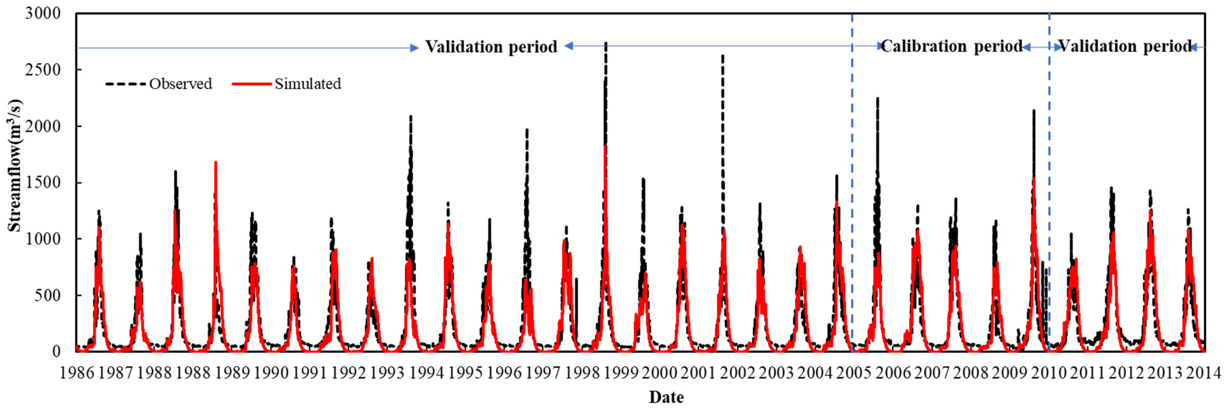
The HEC-HMS model consists of two modules, a rainfall runoff module and a snow and glacier melt module. In the rainfall runoff module, the soil moisture accounting (SMA) loss method, Clark unit hydrograph method, simple canopy method, simple surface method, and the recession method were selected. Monthly evaporation data and the temperature index method based on the ATI-Melt rate function were adopted for evapotranspiration and snowmelt simulations, respectively. In terms of model calibration and validation, an optimization trial and uncertainty simulations were applied in HEC-HMS version 4.2.1 (the latest version), and parameters for runoff, evapotranspiration, snowmelt, groundwater, and soil were optimized accordingly. In this study, the HEC-HMS model was calibrated using data from 2005 to 2010 and validated using data from 1986 to 2004 and 2011–2014 at the outlet of the Yarkant River basin. The results of the optimization of the main parameters in the model are presented in Supplementary Table S2.
The time series of simulated daily streamflow was compared to the observed streamflow using several key statistics, including NSE, R2, and PBIAS (Figure 2, Table 3). These statistics show that the model performed well on a daily time scale during both the calibration and validation periods. NSE for the calibration and validation periods were 0.80, 0.72, and 0.83, respectively, whereas the R2 values for the calibration and validation periods were 0.81, 0.70, and 0.85, respectively. Therefore, model performances over the calibration and validation periods were highly acceptable and can be used in the hydrological simulations.

3.2. Evaluation of Bias Correction Approaches

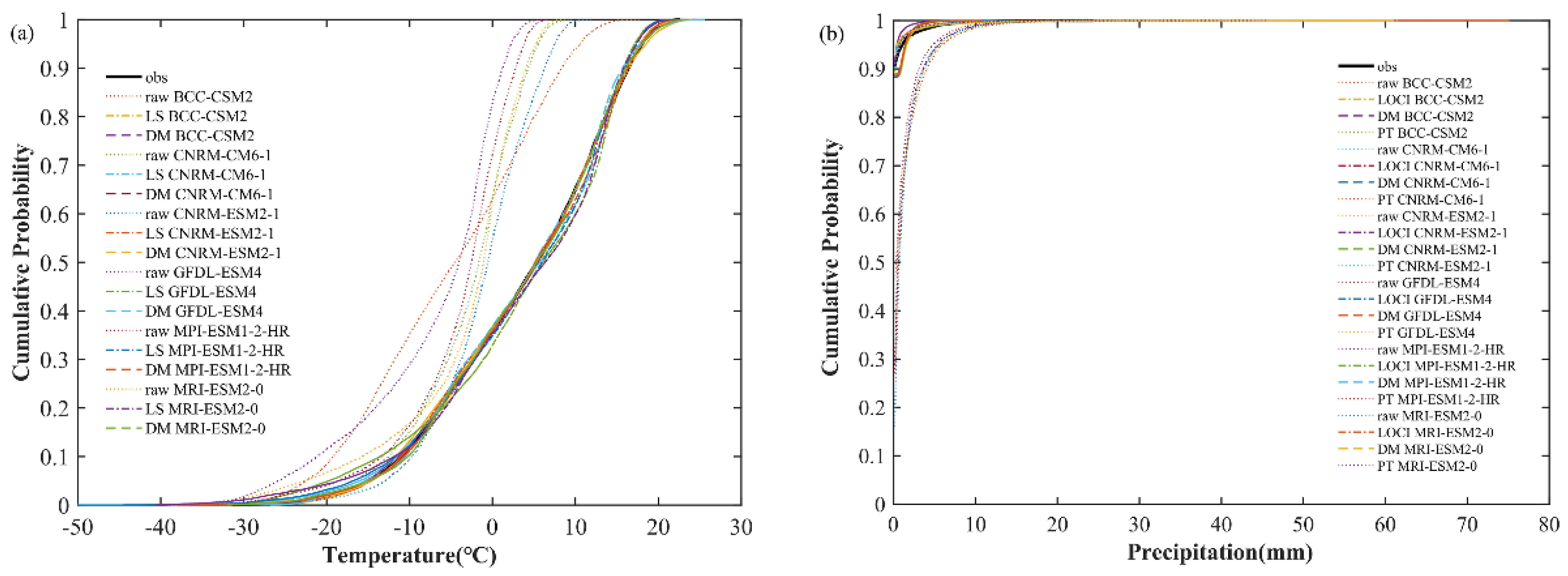
Figure 3 shows the cumulative probability curves for observed, raw, and corrected precipitation and the temperature of six GCMs models listed in Table 1. For temperature, the raw GCM model data underestimates high temperature events (>0 °C) with frequencies above 0.2. The two temperature correction methods applied in this study were able to correct bias for all data, with small differences in effect. For precipitation, all raw GCM model output was overestimated. Regarding the bias correction method, the DM method underestimated precipitation to differing degrees, whereas the LOCI and PT methods overestimated small precipitation events with probabilities less than 0.95. The correction for other precipitation events was better.
The performance of different bias correction approaches in correcting precipitation and temperature was evaluated using both frequency-based statistics and time-series-based metrics over the historical period (1986–2014) (Table 4 and Table 5). In term of temperature, the results show that the mean and standard deviation of temperature at the station were 3.98 °C and 10.06 °C, respectively, whereas the 10% and 90% percentiles were −10.77 °C and 16.70 °C, respectively. The LS and DM methods performed equally well in correcting temperature. Specifically, the LS method provided good estimates of the mean, but slightly overestimated the median and standard deviation, while the DM method provided good estimates of both the frequency-based and time-series-based indicators. These results suggest that the DM method is better at correcting the simulated temperature from the climate model.
In term of precipitation, the average daily precipitation at the meteorological station was 0.23 mm, the annual number of wet days accounted for 5%, and the intensity of wet days was 1.17 mm. All the bias correction methods were effective at improving the simulation efficiency of raw output data, but there was varying degrees of over estimation in both wet day frequency and wet day intensity. Specifically, PT and DM methods overestimated the wet day intensity, and LOCI methods overestimated the wet day frequency, mainly due to the high number of rainfall days in the raw data. The correction methods did not directly eliminate rainfall events. The mean, standard deviation, and wet day frequency of the PT method were similar to the observed values. The RMSE and MAE of the LOCI method were the lowest, but slightly overestimated the wet day frequency, while the RMSE and MAE of the LOCI method were better than other two methods. In general, the LOCI method provided the best correction for precipitation.

3.3. Climate Projections and Climate Change Analysis

3.3.1. Temperature Projection

Based on the evaluation results of the correction methods in the previous section, this study chose the DM method and the LOCI method to correct the raw temperature and precipitation from climate model output of the near future and the far future under the SSP126, SSP245 and SSP370 scenarios. The analysis of changes in climate and hydrologic response was carried out by comparing the near future (2021–2049) and far future (2071–2099) conditions to the control period, 1986–2014. Increased air temperatures were obtained by all climate models under all SSPs (Figure 4a, Table 6). It is clear from the projected results that a basin-wide temperature increase was predicted for both future periods, while the variation trends of temperature during 2015 and 2100 under SSP126, SSP245, and SSP370 were 0.43 °C/10a, 0.49 °C/10a, and 0.73 °C/10a, respectively, with a 95% significance level. However, the uncertainty of the different climate models was large, especially under SSP370. From the perspective of a temperature increase, the difference in the temperature increase between the three pathways was relatively small. The temperature rise for SSP245 (1.79 °C) is expected to be more significant than for SSP126 and SSP370 (1.72 °C, 1.75 °C, respectively). Temperature increased at a similar rate for the three SSPs during the mid-century, while the rate of temperature increase was projected to be rapid during the far future under the three SSPs. The magnitude of the temperature rise under SSP370 was the largest, followed by SSP245 and SSP126 (4.29 °C and 3.76 °C, respectively) (Table 6).
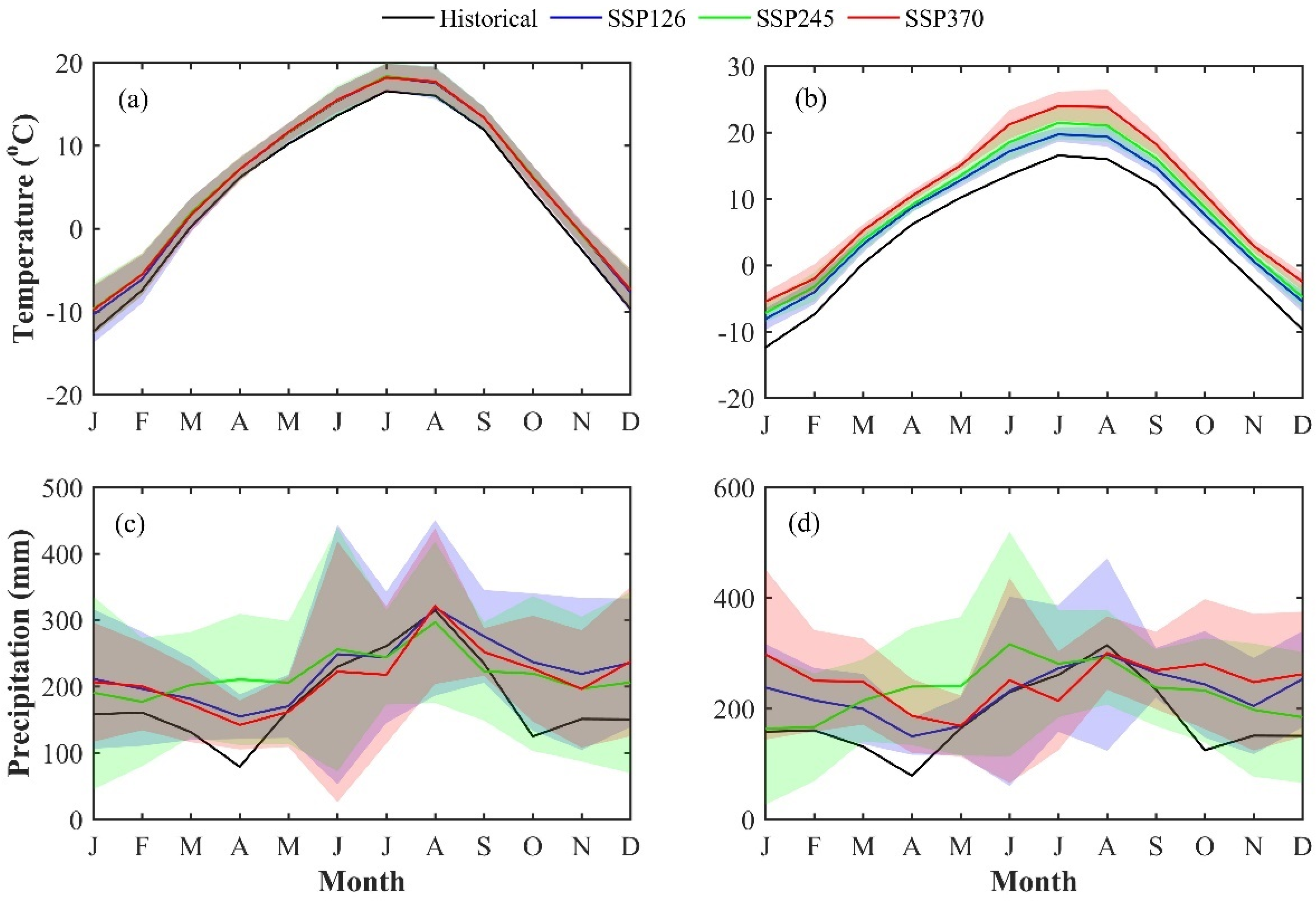
Figure 5a,b show the mean month temperature change under the three SSPs for both near future and far future simulations. Differences in the monthly projected temperature increase between the different SSPs were negligible for the near future period (expect for SSP370) but were substantial for the far future. A comparison of the monthly warming rates shows that both the near- and far-future periods have the highest warming rates during the winter and summer (1.78–6.5 °C and 1.67–7.62 °C, respectively) with greater uncertainty.

3.3.2. Precipitation Projection

Future precipitation is predicted to increase, but the increase differs from the rising trend exhibited by temperature. In contrast to temperature, increases in precipitation do not appear to possess a significant trend, with the rates of at rates of 0.01 mm/10a (p > 0.05), 1.92 mm/10a, and 0.73 mm/10a (p > 0.05), respectively (Figure 4b). In addition, there is more uncertainty in the change in precipitation in the future. In the near future, the increases in precipitation are expected to be 11.95%, 12.00%, and 10.79% under SSP126, SSP245, and SSP370, respectively. For the far future, there was a large difference in the change in precipitation between the three scenarios. The order of increase (from largest to smallest) was SSP370 (29.07%), SSP245 (16.09%), and SSP126 (14.82%).
Seasonally, there will be larger variations in the future, and both the near and far futures will have widespread uncertainty (Figure 5c,d). A significant increase in precipitation was found in autumn and winter (15–113%), while a slight increase or even a decrease in precipitation will occur during the summer (15–113%). It should be noted that the relative increase in precipitation in the dry season was higher than during the wet season, which is similar to climate change scenarios in other arid and semi-arid regions, such as the Kaidu River basin, which originates in the Tien Shan Mountains. Collectively, the findings presented above show that both the annual and monthly average precipitation change in the future will be more uncertain than temperature.

3.4. Streamflow Change Predictions to Changing Climate

3.4.1. Annual and Monthly Streamflow to Changing Climate

Discharge and other hydrological components, such as baseflow and direct flow, obtained from the simulated HEC-HMS model were treated as baseline data for the reference period of 1986 to 2014. The hydrological components obtained from the reference period were compared with the predicted future changes from the six GCMs under the three SSP scenarios.
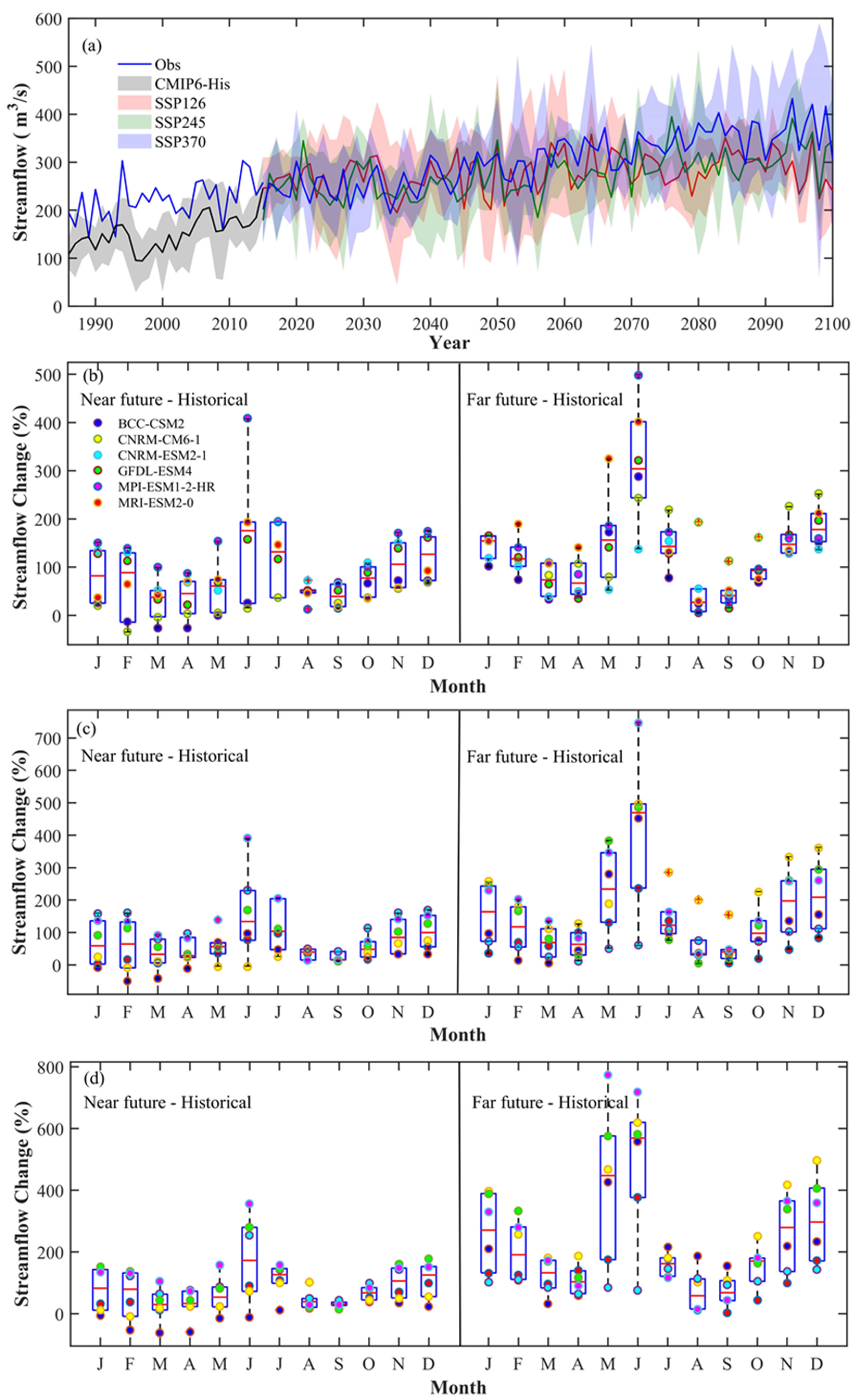
Changes in precipitation and temperature that led to changes in potential streamflow are shown in Table 6. There is a consistent trend in the projected hydrological changes for all the scenarios. Although there are large variations in seasonality and magnitude, the variation trends of streamflow during 2015 and 2100 under SSP126, SSP245, and SSP370 were 4.89 × 10⁸ m3/10a, 4.76 × 10⁸ m3/10a, 8.07 × 10⁸ m3/10a, respectively, with a 95% significance level. Specifically, compared to the control period (1986–2014), the increase in streamflow under SSP126, SSP245, and SSP370 during the near future period was 19.20%, 10.62%, and 14.01%, respectively. The increase in streamflow during the far future period varied greatly among the three scenarios. Ordered from largest to smallest, the results were SSP370 (70.40%), SSP245 (46.11%), and SSP126 (36.69%). It is worth noting that under the scenarios of SSP126 and SSP370, streamflow exhibited a slight decreasing trend at the end of this century (−2.26 × 10⁸ m3/a, −0.17 × 10⁸ m3/a under SSP245 and SSP370, respectively) (Figure 6a), which is consistent with the research findings of Sorg et al. [49], indicating that if the temperature continues to rise, the water shortage in this region is most likely to increase.
The average monthly streamflow change rates under the three different SSP scenarios for the different time periods are shown in Figure 6. Overall, there was an increasing trend in streamflow for all future months, but the increase varies significantly from month to month. In general, the greatest increase in the near- and far futures under the three scenarios are during summer, followed by winter. On a monthly scale, the increase in streamflow was projected to be maximal during June and July during the near future, and during May and June during the far future. In addition, the peak value of streamflow changed from August in the historical period to July in both the near- and far futures (Figure 7).
The range of uncertainty for the change in future projected streamflow is presented in Figure 6. A higher range of uncertainty is associated with a larger difference in the 5th percentile and 95th percentile of the change in streamflow. The winter and summer seasons show the highest certainty. It is particularly high in summer. An analysis of the annual changes in streamflow in the Yarkant River basin during the historical period shows that, due to the seasonal influence of snow and ice meltwater, the monthly flow at the Kaqun station was unevenly distributed during the year. The streamflow from June to September accounted for 80% of the year’s total streamflow. Therefore, the increase in streamflow, combined with the high uncertainty during future floods, will have a significant impact on the ecological and hydrological processes in the basin, causing the hydrological resource system to become more fragile.

3.4.2. Changes in Streamflow Components to Changing Climate

Changes in the contribution of different hydrological components of the hydrological system to changes in climate within the river basin are of high importance. Streamflow can be separated into direct streamflow and baseflow. Baseflow is generally defined as that part of river streamflow coming from groundwater storage and other delayed water inflows [50]. Baseflow is the main source of streamflow during the dry season and is affected by the change of snow and ice meltwater supply [51]. Direct flow means the part of streamflow which enters a stream channel promptly after rainfall or snow melting. This study attempted to simulate changes in major hydrological components (direct streamflow and baseflow) for the future scenario-periods compared to the reference simulated streamflow components (1986–2014) obtained from the HEC-HMS model.
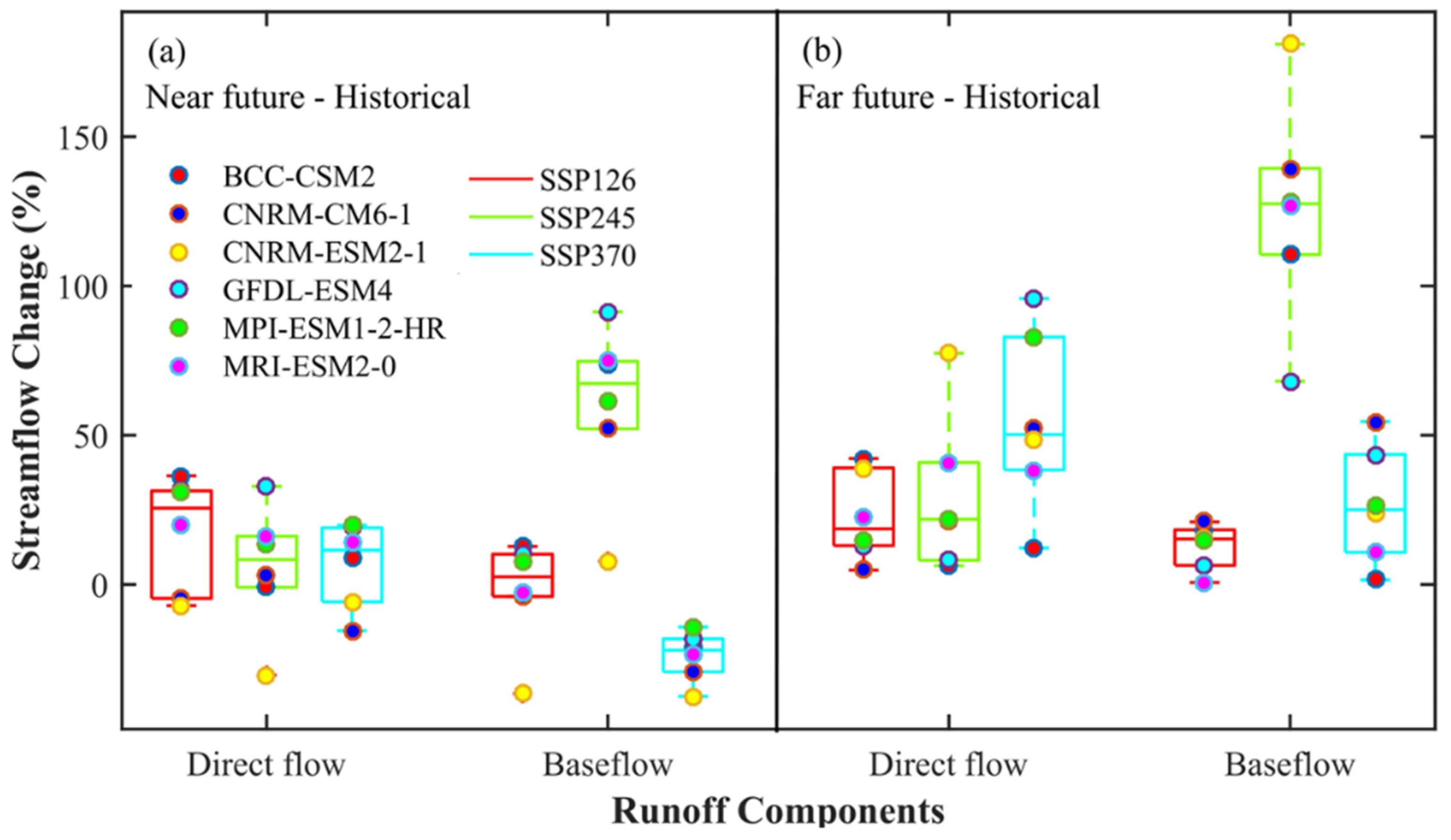
Since observed data for the different hydrological components in the basin were not available, output from the model was used as the baseline or reference data, thereby allowing a comparison of the streamflow components for the future scenarios to the simulated historic values [52]. The simulated baseflow fraction during the simulated historical period is consistent with the research results of Fan et al., suggesting that the streamflow component analysis was reliable [51]. Figure 8 shows that during the near future, direct flow increases by 17.87%, 5.73%, and 6.76% under SSP126, SSP245, and SSP370, respectively, compared with the control period (1986–2014). The change in baseflow was −2.08%, 60.11%, and −23.86%, respectively. During the far future, the increase of direct flow was 22.73%, 29.41%, and 54.97%, and the increase in baseflow was 12.8%, 125.68%, and 26.76%, respectively. The changes and magnitudes of the changes in direct and baseflow are quite different. The changes of direct flow and streamflow are consistent across the different scenarios during the near future period, while baseflow decreases to varying degrees during both scenarios SSP126 and SSP370 over the near future. The magnitudes of the decrease in direct flow and baseflow varied during the far future. The increase of baseflow in the two future periods under both the SSP126 and SSP370 scenarios is much lower than under the SSP245 scenario.

3.4.3. Extreme Flows

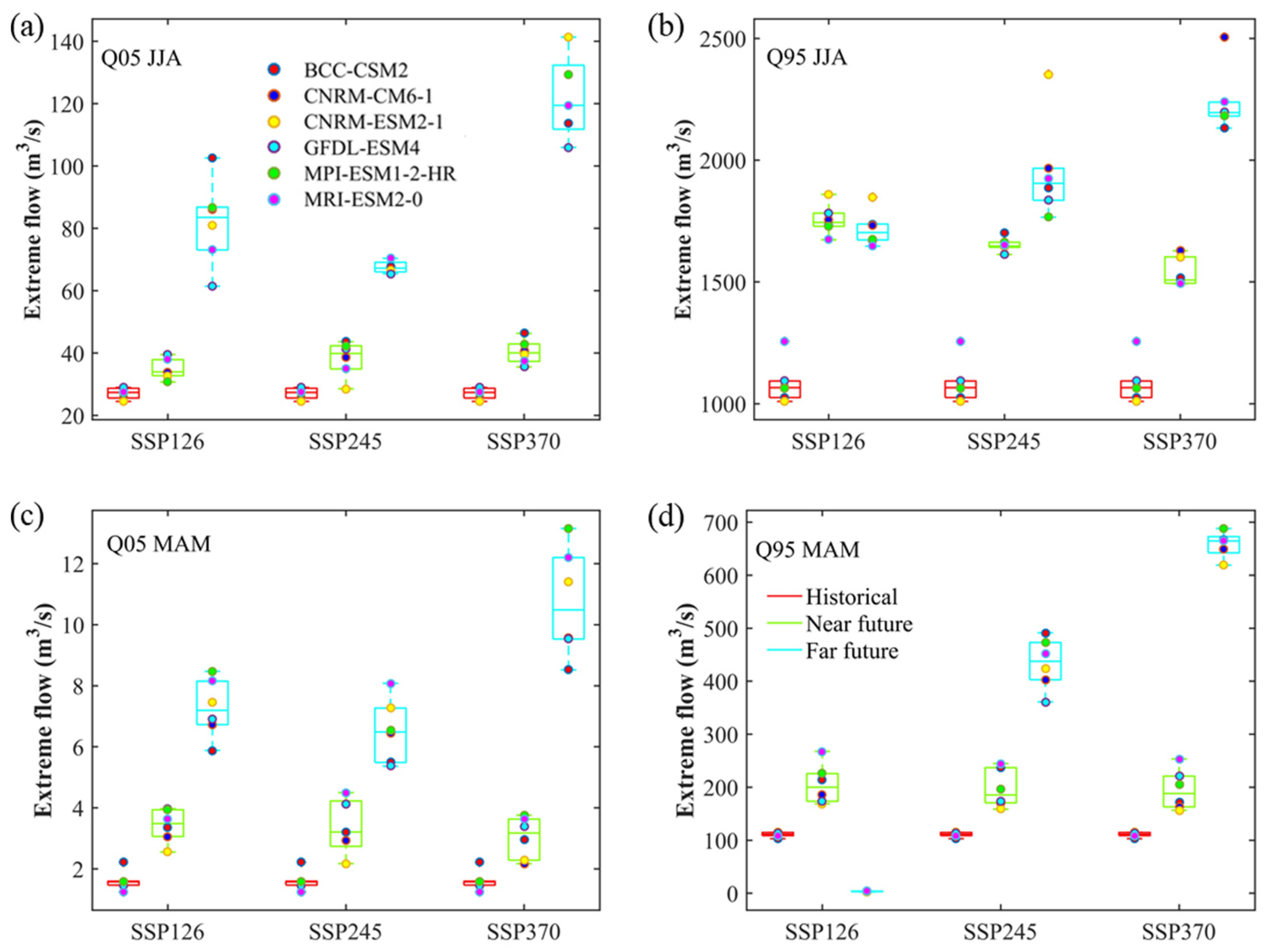
Both upstream streamflow generation in Yarkant River basin and ecological and domestic water consumption in downstream areas of the basin are concentrated during the spring and summer months [3,17]. Thus, extreme flows, including the low flow (Q5) and high flow (Q95) magnitudes (Figure 9), as well as the number of days of low and high flow occurrence (Figure 10) during the spring (March–May, MAM) and summer (June-August, JJA) of the historical period and the two future periods, were analyzed. Q95 and Q5 were computed herein based on mean streamflow for the six simulations. Figure 9 shows that low flows (Q5) for JJA and MAM increased during both the near future and the far future periods under the three SSP scenarios. However, there was a more dramatic increase during the far future period. High flows (Q95) exhibited an increasing pattern under all but the SSP126 scenario. The JJA and MAM seasons for all three periods of the scenario also show a consistent increasing trend. In contrast, the SSP126 scenario shows a trend of increasing and then decreasing high flows (Q95) from the historical period to the near future period, and then to the far future period. Overall, both low flows and high flows will increase in the future to varying degrees during the spring and summer.
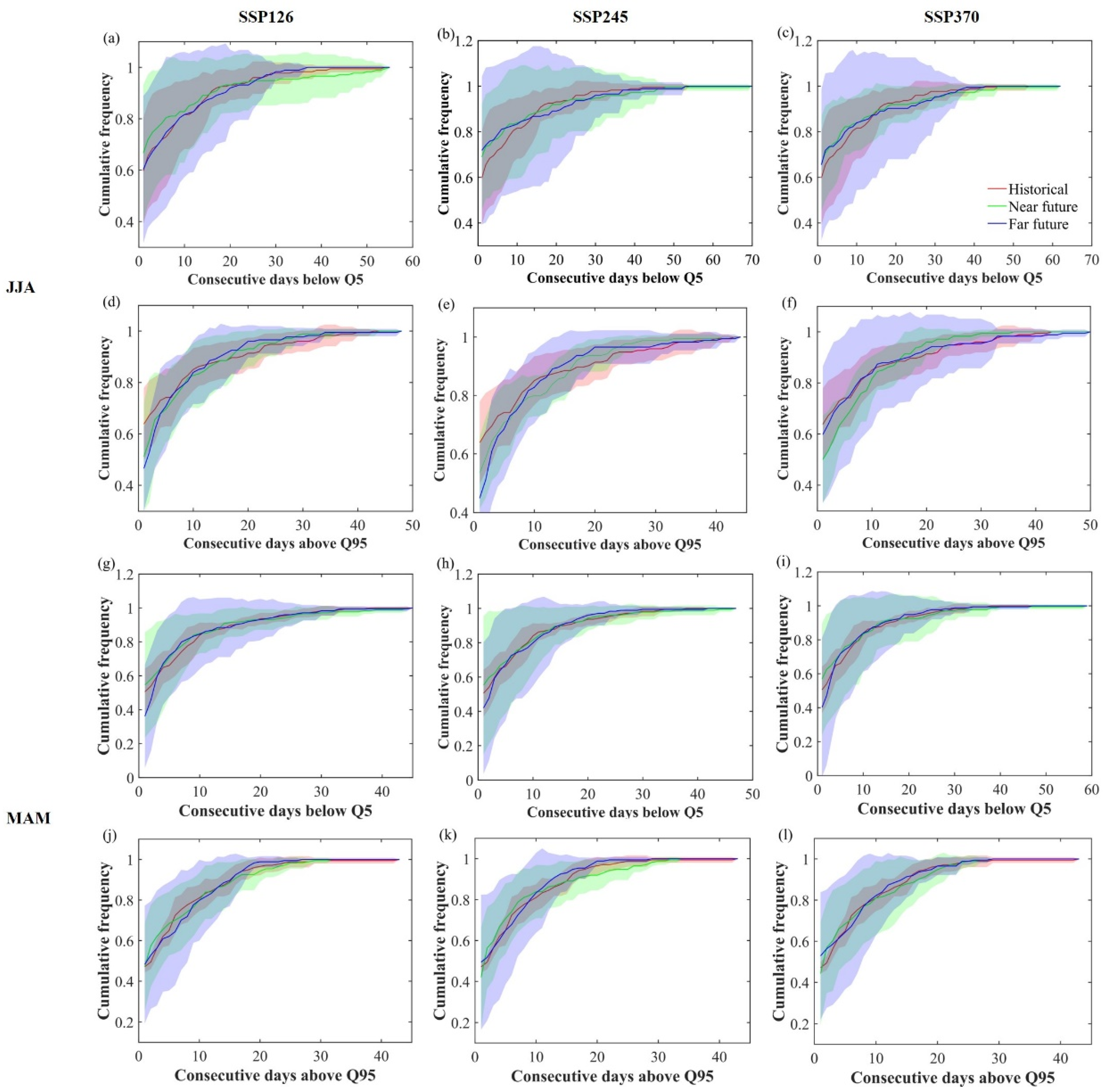
The frequency of consecutive days below Q5 is expected to decrease under the influence of climate change in JJA. Figure 10 demonstrates this concept by showing the cumulative distribution functions (CDFs) of the consecutive days below Q5 for the Yarkant catchment over the MAM and JJA seasons. A threshold of about 15 days exists for calculating changes in streamflow for the historical and two future periods, where the probability of low flow occurring for less than 15 days in the summer will be higher than that in the historical period. The probability of greater than 15 days will be lower than during the historical period. For high flows, the opposite is true. The probability of high flows occurring for less than 15 days during the summer in the future will be lower than in the historical period, and the probability of greater than 15 days will be higher than during the historical period. In other words, in regard to extreme summer hydrologic events in the future, there are relatively fewer extended periods of low flow, and relatively more extended periods of high flow in JJA. As such, there will be fewer prolonged drought events triggered by low flows and more flood events triggered by high flows. The future CDFs for low flow days in MAM will not change significantly. The probability of the occurrence of low flow days greater than 15 days will be slightly higher than that in the historical period. The change in high flow days will be relatively complex during the far future. The probability of high flow occurring for more than 15 days will be higher in the far future, while in the near future lower than during the historical period. Put differently, there will be more extended periods of low spring flows, and the frequency of drought events triggered by low flow will increase during the spring in the future. In general, the frequency of spring droughts and summer floods will increase in the future, and the risk of extreme hydrological events in spring and summer will also increase. These changes will pose greater challenges to agricultural water allocation and water resources management in the oasis of the lower Yarkant River basin.

4. Discussion

4.1. Application of Hydrological Model

In arid areas where there is a lack of observational data, a distributed hydrological model with certain physical significance based on the degree-day factor is more suitable [53,54]. Therefore, this study used the HEC-HMS model combined with the improved ATIMR parameters. The approach comprehensively considers glacier or snow degree-day factors, melt temperature, glacier area, and snow water equivalent, among other parameters, to effectively improve the efficiency and accuracy of model calibration.
Remote sensing re-analysis data are limited by spatial resolution and were thus difficult to use in this study. Accordingly, we used lapse rate interpolation to differentiate elevation zones. The use of a constant lapse rate often does not describe mountainous watersheds well [55]. In this study, we thus used monthly temperature decline rate when simulating runoff.
In addition, the study selected the utilized temperature and precipitation data because the snow and glacier melting module in HEC-HMS is mainly based on temperature, and the change of runoff is sensitive to both temperature and precipitation [56]. In the currently published CMIP6 climate model, snow water equivalent, relative humidity, and other data are still scarce. In future studies, additional climate data and variables can be used to predict future changes in multiple climate elements and the resulting changes in hydrological processes.

4.2. The Applicability of CMIP6 Models and Bias Correction Methods in the Arid Area of Northwest China

The CMIP6 model maintains a good interface with CMIP5 and considers more complex processes. Many of its component models achieve bidirectional coupling of atmospheric chemical processes, and the resolution of atmospheric and oceanic models is significantly higher, which is an improvement and extension of the CMIP5 model [42,57,58]. In this study, three SSP scenarios and six climate models incorporating these three scenarios were selected and applied to the Yarkant River basin located in the arid area of northwest China. An evaluation of the corrected model data shows that these models simulate watershed temperatures well, which is consistent with the evaluations of the CMIP6 model by other investigators [59]. While there is some error in the low precipitation events and precipitation intensities, which is a common feature of global climate models [60,61]. In general, the six CMIP6 models used in this study have relatively reliable applicability in the arid area of northwest China.
It is also worth noting that bias correction methods are usually considered to be another contributor of uncertainty in climate change impact studies [48,62]. This study chose bias correction methods by comparing the effectiveness of two temperature bias correction methods and three precipitation bias correction methods to reduce uncertainty. The different bias correction methods, shown in Section 3.3.1, worked well for temperature but not as well for precipitation. For arid regions, the errors in the precipitation model are mainly in the frequency of precipitation. The LOCI method applied in this study performed the best, and therefore is recommended for use as the method for correcting precipitation bias from climate models in arid regions.
The IPCC Fifth Assessment Report (AR5) (IPCC, 2018) shows that the range in temperature rise of the different emission scenarios (RCP2.6, RCP 4.5, RCP 8.5) from 2046 to 2065 is within about 2 °C, while that between 2081 and 2100 is different. This is especially true for RCP8.5, in which increases in temperature reach 3.7 ± 7 °C, which is consistent with the change in temperature projected in this study. Future changes in climate are thought to be strongly spatially heterogeneous. The arid region of northwest China, located in the hinterland of Eurasia in the middle latitude of the northern hemisphere, is highly sensitive to global climate change [63,64]. The results of the CMIP5 multimodal projection of future temperature in China show that larger relative increases are projected for inland regions, especially the northwest [65]. Taking RCP8.5 as an example, by the end of the 21st century (2081–2100), the annual mean SAT averaged over northwest China increased by 5.5 °C [66]. The results of the latest CMIP6 climate model also show that there is a tendency for an increase in both temperature and precipitation in the future. The annual mean temperature is projected to increase at rates of 0.06 °C, 0.26 °C, and 0.59 °C per decade under SSP126, SSP245, and SSP585, respectively [67]. In this study, the range of predicted future warming is consistent with research results mentioned above. Future climate change and its impact on hydrological and ecological issues in this climatically sensitive area requires more attention.

4.3. Climate Change Impacts on Runoff

The effects of climate change on runoff during historical periods have been extensively studied, especially in climate-sensitive regions, including: (1) central Asia and the arid regions of northwest China, where runoff is highly sensitive to changes in temperature and precipitation, and (2) in mountainous watersheds where the proportion of glacial snowmelt in runoff varies, leading to greater differences in hydrological characteristics [68,69,70]. In this study, a simple correlation analysis between temperature, precipitation, and runoff under different SSP scenarios showed that the correlation coefficient of runoff with precipitation under SSP126 (0.50) was higher than that with temperature (0.49). In contrast, the correlation coefficient of runoff with temperature under SSP245 and SSP370 (0.74, 0.87) was higher than that with precipitation (0.63, 0.76), which mainly results from the higher temperature under the higher carbon emissions scenario, resulting in more glacial and snow meltwater and increased runoff.
The study also found that there are obvious seasonal differences in the predicted future runoff changes, with the greatest increase in runoff occurring in summer followed by winter. Unlike precipitation-replenished watershed runoff, runoff in the Yarkant River basin is mainly recharged by glacier and snow meltwater, which is concentrated in summer. Changes in runoff are most significantly influenced by temperature. A predicted future temperature increase of 1.67–7.62 °C would result in a 6.02–51.72% increase in summer runoff. Basins with headwaters originating in the Himalayas, Karakoram, and the Tien Shan region also showed a similar relationship [71,72,73]. Summer precipitation did not increase or decrease in the Yarkant River basin. Runoff was less affected by changes in precipitation, a finding that differs from other dryland snowmelt-rainfall recharge watersheds [74]. The winter flows seem to vary under the dual effect of temperature and precipitation. From the analysis of estimated future monthly runoff changes, it was found that the incremental maximum of the near-future runoff was in June–July, while the incremental maximum of the far-future runoff was in May–June. The peak runoff period changed from August to July, which may be because rising temperatures lead to earlier snow- and ice-melt, which in turn leads to earlier peak runoff. The spring droughts and summer floods that currently exist in the watershed are likely to become more pronounced and severe in the future, thus requiring more attention to water resources planning and management in the watershed.

5. Conclusions

The hydrological regimes of basins in arid areas are vulnerable to climatic variations, especially precipitation and temperature. In our study, we examined the impact of climate change on climate variables (temperature and precipitation), runoff, and major runoff components (direct flow and baseflow) in a typical arid inland river (Yarkant River basin) using data from the latest CMIP6 models. The HEC-HMS model was used to predict future changes in the hydrological regime of the Yarkant Basin based on three SSPs (SSP126, SSP245, and SSP370) of the downscaled latest Coupled Model Intercomparison Project’s (CMIP6) General Circulation Model outputs.
The DM and LOCI bias correction approaches performed the best in the projections of temperature and precipitation, respectively. Temperature was predicted to increase by 1.72–1.79 °C during the near future and by 3.76–6.22 °C during the far future. Precipitation will increase by 10.79–12% and 14.82–29.07% during the near future and far future, respectively, in comparison to 1986–2014. Future changes in precipitation are more complex, with less significant changes than temperature but greater uncertainties, especially in summer and winter.
Changes in temperature and precipitation lead to changes in hydrological regimes. Runoff was projected to have a consistent trend for all the scenarios, although there are large variabilities regarding seasonality and magnitude. Moreover, the increase in direct flow was projected to be greater than baseflow, except under SSP245 conditions. Seasonally, the increase in runoff was the greatest in summer and winter, as was the uncertainty. An increase in runoff was projected to be maximal in June and July during the near future, while occurring in May and June during the far future. Peak runoff will also change from August during the historical period to July. Both high- and low-flow magnitude in MAM and JJA will increase by varying degrees. There are likely to be relatively fewer extended periods of low flow and relatively more extended periods of high flow in JJA. While there are relatively more extended periods of low flow in MAM, the frequency of spring droughts and summer floods will further increase in the future, which will increase the risk of extreme hydrological events in spring and summer.
In general, future warming and precipitation changes in the study basin are evident, as is an increase in mountain runoff due to climate change. However, the increase in extreme climatic and hydrological events due to climatic and hydrological uncertainties will be hard to ignore, which poses new challenges for water resources management in the basin.

Supplementary Materials

The following supporting information can be downloaded at: https://www.mdpi.com/article/10.3390/rs14010115/s1, Table S1: Precipitation lapse rate of each month in Yarkant River basin; Table S2: Estimated and calibrated Parameters for the calibration and validation of streamflow, for the six sub-basins of Yarkant River basin. References [33,75,76,77] are cited in the supplementary materials.

Author Contributions

Conceptualization, Y.X., Q.Z., and Y.W.; funding acquisition, Y.W. and Y.C.; data curation, Y.X.; methodology, Y.X. and Q.Z.; software, Y.X. and Q.Z.; formal analysis, Y.X.; investigation, Y.X.; project administration, Y.W.; resources, Y.X.; validation, Y.W. and Q.Z.; writing—original draft, Y.X.; writing—review and editing, Q.Z. and Y.W. All authors have read and agreed to the published version of the manuscript.

Funding

The research is supported by the National Natural Science Foundation of China (52161145102); Guangdong Foundation for Program of Science and Technology Research (2020B1111530001, 2019QN01L682).

Institutional Review Board Statement

Not applicable.

Informed Consent Statement

Not applicable.

Data Availability Statement

Daily snow depth can be found at http://data.tpdc.ac.cn (accessed on 18 November 2021); the First and Second Glacier Inventory Dataset of China and the Randolph Glacier In-ventory (RGI 6.0) can be found at https://doi.org/10.7265/N5-RGI-60 (accessed on 18 November 2021); Soils datasat are provided by http://www.bdc.ac.cn/portal/ (accessed on 18 November 2021).

Acknowledgments

We thank LetPub (www.letpub.com accessed on 18 November 2021) for its linguistic assistance and scientific consultation during the preparation of this manuscript.

Conflicts of Interest

The authors declare no conflict of interest.

References

  1. Müller Schmied, H.; Adam, L.; Eisner, S.; Fink, G.; Flörke, M.; Kim, H.; Oki, T.; Portmann, F.T.; Reinecke, R.; Riedel, C.; et al. Variations of global and continental water balance components as impacted by climate forcing uncertainty and human water use. Hydrol. Earth Syst. Sci. 2016, 20, 2877–2898. [Google Scholar] [CrossRef] [Green Version]
  2. Han, H.; Wang, R. Landscape pattern change research of Yarkant irrigated area. In Proceedings of the 2012 International Symposium on Geomatics for Integrated Water Resource Management, Lanzhou, China, 19–21 October 2012; pp. 1–4. [Google Scholar]
  3. Huang, S.; Wortmann, M.; Duethmann, D.; Menz, C.; Shi, F.; Zhao, C.; Su, B.; Krysanova, V. Adaptation strategies of agriculture and water management to climate change in the Upper Tarim River basin, NW China. Agric. Water Manag. 2018, 203, 207–224. [Google Scholar] [CrossRef]
  4. Xiang, Y.; Wang, Y.; Chen, Y.; Bai, Y.; Zhang, L.; Zhang, Q. Hydrological Drought Risk Assessment Using a Multidimensional Copula Function Approach in Arid Inland Basins, China. Water 2020, 12, 1888. [Google Scholar] [CrossRef]
  5. Xu, J.; Chen, Y.; Li, W.; Nie, Q.; Song, C.; Wei, C. Integrating Wavelet Analysis and BPANN to Simulate the Annual Runoff With Regional Climate Change: A Case Study of Yarkand River, Northwest China. Water Resour. Manag. 2014, 28, 2523–2537. [Google Scholar] [CrossRef]
  6. Held, I.M.; Soden, B.J. Robust Responses of the Hydrological Cycle to Global Warming. J. Clim. 2006, 19, 5686–5699. [Google Scholar] [CrossRef]
  7. Barnett, T.P.; Adam, J.C.; Lettenmaier, D.P. Potential impacts of a warming climate on water availability in snow-dominated regions. Nature 2005, 438, 303–309. [Google Scholar] [CrossRef]
  8. Lutz, A.F.; Immerzeel, W.W.; Shrestha, A.B.; Bierkens, M.F.P. Consistent increase in High Asia’s runoff due to increasing glac-ier melt and precipitation. Nat. Clim. Chang. 2014, 4, 587–592. [Google Scholar] [CrossRef] [Green Version]
  9. Ragettli, S.; Immerzeel, W.W.; Pellicciotti, F. Contrasting climate change impact on river flows from high-altitude catch-ments in the Himalayan and Andes Mountains. Proc. Natl. Acad. Sci. USA 2016, 113, 6. [Google Scholar] [CrossRef] [PubMed] [Green Version]
  10. Sun, C.; Yang, J.; Chen, Y.; Li, X.; Yang, Y.; Zhang, Y. Comparative study of streamflow components in two inland rivers in the Tianshan Mountains, Northwest China. Environ. Earth Sci. 2016, 75, 9. [Google Scholar] [CrossRef]
  11. Bi, Y.; Hongjie, X.; Chunlin, H.; Changqing, K. Snow Cover Variations and Controlling Factors at Upper Heihe River Basin, Northwestern China. Remote Sens. 2015, 7, 6741–6762. [Google Scholar] [CrossRef] [Green Version]
  12. Wang, W.; Huang, X.; Deng, J.; Xie, H.; Liang, T. Spatio-Temporal Change of Snow Cover and Its Response to Climate over the Tibetan Plateau Based on an Improved Daily Cloud-Free Snow Cover Product. Remote Sens. 2015, 7, 169–194. [Google Scholar] [CrossRef]
  13. Tobias, S.; Thomas, B.; Renaud, G.; Scott, S.; Andrew, W.R.; Justin, M.; Peter, B.-G.; Andrey, Y. Will climate change exacerbate water stress in? Clim. Chang. 2012, 122, 881–899. [Google Scholar]
  14. Chen, F.; Chen, Y.; Bakhtiyorov, Z.; Zhang, H.; Man, W.; Chen, F. Central Asian river streamflows have not continued to increase during the recent warming hiatus. Atmos. Res. 2020, 246, 105–124. [Google Scholar] [CrossRef]
  15. Tosunoğlu, F.; Onof, C. Joint modelling of drought characteristics derived from historical and synthetic rainfalls: Application of Generalized Linear Models and Copulas. J. Hydrol.—Reg. Stud. 2017, 14, 167–181. [Google Scholar] [CrossRef]
  16. Zhang, S.; Gao, X.; Zhang, X.; Hagemann, S. Projection of glacier runoff in Yarkant River basin and Beida River basin, Western China. Hydrol. Processes 2012, 26, 2773–2781. [Google Scholar] [CrossRef]
  17. Luo, Y.; Wang, X.; Piao, S.; Sun, L.; Ciais, P.; Zhang, Y.; Ma, C.; Gan, R.; He, C. Contrasting streamflow regimes induced by melting glaciers across the Tien Shan—Pamir—North Karakoram. Sci. Rep. 2018, 8, 16470. [Google Scholar] [CrossRef] [PubMed]
  18. Azmat, M.; Qamar, M.U.; Huggel, C.; Hussain, E. Future climate and cryosphere impacts on the hydrology of a scarcely gauged catchment on the Jhelum river basin, Northern Pakistan. Sci. Total Environ. 2018, 639, 961–976. [Google Scholar] [CrossRef]
  19. Li, S.-Y.; Miao, L.-J.; Jiang, Z.-H.; Wang, G.-J.; Gnyawali, K.R.; Zhang, J.; Zhang, H.; Fang, K.; He, Y.; Li, C. Projected drought conditions in Northwest China with CMIP6 models under combined SSPs and RCPs for 2015–2099. Adv. Clim. Chang. Res. 2020, 11, 210–217. [Google Scholar] [CrossRef]
  20. Chen, Y.; Li, W.; Fang, G.; Li, Z. Review article: Hydrological modeling in glacierized catchments of central Asia—status and challenges. Hydrol. Earth Syst. Sci. 2017, 21, 669–684. [Google Scholar] [CrossRef] [Green Version]
  21. U.S. Army Corps of Enginers Hydrologic Engineering Center. Hydrologic Modeling System HEC-HMS User’s Manual; US Army Corps of Engineers, Hydrologic Engineering Center: Davis, CA, USA, 2016. [Google Scholar]
  22. Azmat, M.; Choi, M.; Kim, T.-W.; Liaqat, U.W. Hydrological modeling to simulate streamflow under changing climate in a scarcely gauged cryosphere catchment. Environ. Earth Sci. 2016, 75, 186. [Google Scholar] [CrossRef]
  23. Fazel, K.; Scharffenberg, W.A.; Bombardelli, F.A. Assessment of the Melt Rate Function in a Temperature Index Snow Model Using Observed Data. J. Hydrol. Eng. 2014, 19, 1275–1282. [Google Scholar] [CrossRef]
  24. Konapala, G.; Mishra, A.K.; Wada, Y.; Mann, M.E. Climate change will affect global water availability through compounding changes in seasonal precipitation and evaporation. Nat. Commun. 2020, 11, 3044. [Google Scholar] [CrossRef] [PubMed]
  25. Laurent, L.; Buoncristiani, J.-F.; Pohl, B.; Zekollari, H.; Farinotti, D.; Huss, M.; Mugnier, J.-L.; Pergaud, J. The impact of climate change and glacier mass loss on the hydrology in the Mont-Blanc massif. Sci. Rep. 2020, 10, 10420. [Google Scholar] [CrossRef]
  26. Xu, Y.; Zhang, X.; Wang, X.; Hao, Z.; Singh, V.P.; Hao, F. Propagation from meteorological drought to hydrological drought under the impact of human activities: A case study in northern China. J. Hydrol. 2019, 579, 124147. [Google Scholar] [CrossRef]
  27. Chen, Y.; Liu, A.; Zhang, Z.; Hope, C.; Crabbe, M.J.C. Economic losses of carbon emissions from circum-Arctic permafrost regions under RCP-SSP scenarios. Sci. Total Environ. 2019, 658, 1064–1068. [Google Scholar] [CrossRef]
  28. Moss, R.H.; Edmonds, J.A.; Hibbard, K.A.; Manning, M.R.; Rose, S.K.; van Vuuren, D.P.; Carter, T.R.; Emori, S.; Kainuma, M.; Kram, T. The next generation of scenarios for climate change research and assessment. Nature 2010, 463, 747–756. [Google Scholar] [CrossRef] [PubMed]
  29. Almazroui, M.; Saeed, F.; Saeed, S.; Nazrul Islam, M.; Ismail, M.; Klutse, N.A.B.; Siddiqui, M.H. Projected Change in Temperature and Precipitation Over Africa from CMIP6. Earth Syst. Environ. 2020, 4, 455–475. [Google Scholar] [CrossRef]
  30. Parsons, L.A. Implications of CMIP6 Projected Drying Trends for 21st Century Amazonian Drought Risk. Earth’s Future 2020, 8, e2020EF001608. [Google Scholar] [CrossRef]
  31. Church, J.A.; Clark, P.U.; Cazenave, A.; Gregory, J.M.; Jevrejeva, S.; Levermann, A.; Merrifield, M.A.; Milne, G.A.; Nerem, R.S.; Nunn, P.D.; et al. Sea Level Change. In Climate Change 2013: The Physical Science Basis. Contribution of Working Group I to the Fifth Assessment Report of the Intergovernmental Panel on Climate Change; Stocker, T.F., Qin, D., Plattner, G.-K., Tignor, M., Allen, S.K., Boschung, J., Nauels, A., Xia, Y., Bex, V., Midgley, P.M., Eds.; Cambridge University Press: Cambridge, UK; New York, NY, USA, 2013; Volume 26, pp. 1137–1216. [Google Scholar]
  32. O’Neill, B.C.; Kriegler, E.; Riahi, K.; Ebi, K.L.; Hallegatte, S.; Carter, T.R.; Mathur, R.; van Vuuren, D.P. A new scenario framework for climate change research: The concept of shared socioeconomic pathways. Clim. Change 2013, 122, 387–400. [Google Scholar] [CrossRef] [Green Version]
  33. Kan, B.; Su, F.; Xu, B.; Xie, Y.; Li, J.; Zhang, H. Generation of High Mountain Precipitation and Temperature Data for a Quantitative Assessment of Flow Regime in the Upper Yarkant Basin in the Karakoram. J. Geophys. Res. Atmos. 2018, 123, 8462–8486. [Google Scholar] [CrossRef]
  34. Chen, Y.; Xu, C.; Chen, Y.; Li, W.; Liu, J. Response of glacial-lake outburst floods to climate change in the Yarkant River basin on northern slope of Karakoram Mountains, China. Quat. Int. 2010, 226, 75–81. [Google Scholar] [CrossRef]
  35. Li, B.; Chen, Y.; Chipman, J.W.; Shi, X.; Chen, Z. Why does the runoff in Hotan River show a slight decreased trend in northwestern China? Atmos. Sci. Lett. 2018, 19, e800. [Google Scholar] [CrossRef] [Green Version]
  36. Che, T.; Xin, L.; Jin, R.; Armstrong, R.; Zhang, T. Snow depth derived from passive microwave remote-sensing data in China. Ann. Glaciol. 2008, 49, 145–154. [Google Scholar] [CrossRef] [Green Version]
  37. Dai, L. Inter-Calibrating SMMR, SSM/I and SSMI/S Data to Improve the Consistency of Snow-Depth Products in China. Remote Sens. 2015, 7, 7212–7230. [Google Scholar] [CrossRef] [Green Version]
  38. Liyun, D.; Tao, C.; Yongjian, D.; Xiaohua, H. Evaluation of snow cover and snow depth on the Qinghai–Tibetan Plateau derived from passive microwave remote sensing. Cryosphere 2017, 11, 1933–1948. [Google Scholar]
  39. Redding, D.W.; Atkinson, P.M.; Cunningham, A.A.; Lo Iacono, G.; Moses, L.M.; Wood, J.L.N.; Jones, K.E. Impacts of environmental and socio-economic factors on emergence and epidemic potential of Ebola in Africa. Nat. Commun. 2019, 10, 4531. [Google Scholar] [CrossRef]
  40. O’Neill, B.C.; Kriegler, E.; Ebi, K.L.; Kemp-Benedict, E.; Riahi, K.; Rothman, D.S.; van Ruijven, B.J.; van Vuuren, D.P.; Birkmann, J.; Kok, K.; et al. The roads ahead: Narratives for shared socioeconomic pathways describing world futures in the 21st century. Glob. Environ. Chang. 2017, 42, 169–180. [Google Scholar] [CrossRef] [Green Version]
  41. Chen, Y.; Li, X.; Huang, K.; Luo, M.; Gao, M. High-Resolution Gridded Population Projections for China Under the Shared Socioeconomic Pathways. Earth’s Future 2020, 8, e2020EF001491. [Google Scholar] [CrossRef]
  42. O’Neill, B.C.; Tebaldi, C.; van Vuuren, D.P.; Eyring, V.; Friedlingstein, P.; Hurtt, G.; Knutti, R.; Kriegler, E.; Lamarque, J.-F.; Lowe, J.; et al. The Scenario Model Intercomparison Project (ScenarioMIP) for CMIP6. Geosci. Model Dev. 2016, 9, 3461–3482. [Google Scholar] [CrossRef] [Green Version]
  43. Halwatura, D.; Najim, M.M.M. Application of the HEC-HMS model for runoff simulation in a tropical catchment. Environ. Modell. Softw. 2013, 46, 155–162. [Google Scholar] [CrossRef]
  44. Tassew, B.G.; Belete, M.A.; Miegel, K. Application of HEC-HMS Model for Flow Simulation in the Lake Tana Basin: The Case of Gilgel Abay Catchment, Upper Blue Nile Basin, Ethiopia. Hydrology 2019, 6, 21. [Google Scholar] [CrossRef] [Green Version]
  45. Meenu, R.; Rehana, S.; Mujumdar, P.P. Assessment of hydrologic impacts of climate change in Tunga-Bhadra river basin, India with HEC-HMS and SDSM. Hydrol. Process. 2013, 27, 1572–1589. [Google Scholar] [CrossRef]
  46. Zhao, Q.; Zhang, S.; Ding, Y.J.; Wang, J.; Han, H.; Xu, J.; Zhao, C.; Guo, W.; Shangguan, D. Modeling Hydrologic Response to Climate Change and Shrinking Glaciers in the Highly Glacierized Kunma Like River Catchment, Central Tian Shan. J. Hydrometeorol. 2015, 16, 2383–2402. [Google Scholar] [CrossRef]
  47. Moriasi, D.N.; Arnold, J.G.; Van Liew, M.W.; Bingner, R.L.; Harmel, R.D.; Veith, T.L. Model evaluation guidelines for systematic quantification of accuracy in watershed simulations. Trans. ASABE 2007, 50, 885–900. [Google Scholar] [CrossRef]
  48. Li, L.; Shen, M.; Hou, Y.; Xu, C.-Y.; Lutz, A.F.; Chen, J.; Jain, S.K.; Li, J.; Chen, H. Twenty-first-century glacio-hydrological changes in the Himalayan headwater Beas River basin. Hydrol. Earth Syst. Sci. 2019, 23, 1483–1503. [Google Scholar] [CrossRef] [Green Version]
  49. Sorg, A.; Bolch, T.; Stoffel, M.; Solomina, O.; Beniston, M. Climate change impacts on glaciers and runoff in Tien Shan (Central Asia). Nat. Clim. Change 2012, 2, 725–731. [Google Scholar] [CrossRef]
  50. Hall, F.R. Base flow recessions—A review. Water Resour. Res. 1968, 4, 973–983. [Google Scholar] [CrossRef]
  51. Fan, Y.; Chen, Y.; Liu, Y.; Li, W. Variation of baseflows in the headstreams of the Tarim River Basin during 1960–2007. J. Hydrol. 2013, 487, 98–108. [Google Scholar] [CrossRef]
  52. Viola, M.R.; de Mello, C.R.; Chou, S.C.; Yanagi, S.N.; Gomes, J.L. Assessing climate change impacts on Upper Grande River Basin hydrology, Southeast Brazil. Int. J. Climatol. 2015, 35, 1054–1068. [Google Scholar] [CrossRef]
  53. Kong, X.; Li, Z.; Liu, Z. Flood Prediction in Ungauged Basins by Physical-Based TOPKAPI Model. Adv. Meteorol. 2019, 2019, 4795853. [Google Scholar] [CrossRef]
  54. Wi, S.; Yang, Y.C.E.; Steinschneider, S.; Khalil, A.; Brown, C.M. Calibration approaches for distributed hydrologic models in poorly gaged basins: Implication for streamflow projections under climate change. Hydrol. Earth Syst. Sci. 2015, 19, 857–876. [Google Scholar] [CrossRef] [Green Version]
  55. Fang, G.; Yang, J.; Chen, Y.; Li, Z.; Ji, H.; De Maeyer, P. How Hydrologic Processes Differ Spatially in a Large Basin: Multisite and Multiobjective Modeling in the Tarim River Basin. J. Geophys. Res. Atmos. 2018, 123, 7079–7113. [Google Scholar] [CrossRef]
  56. Zhang, F.; Bai, L.; Li, L.; Wang, Q. Sensitivity of runoff to climatic variability in the northern and southern slopes of the Middle Tianshan Mountains, China. J. Arid Land 2016, 8, 681–693. [Google Scholar] [CrossRef] [Green Version]
  57. Parsons, L.A.; Brennan, M.K.; Wills, R.C.J.; Proistosescu, C. Magnitudes and Spatial Patterns of Interdecadal Temperature Variability in CMIP6. Geophys. Res. Lett. 2020, 47, e2019GL086588. [Google Scholar] [CrossRef]
  58. Xin, X.; Wu, T.; Zhang, J.; Yao, J.; Fang, Y. Comparison of CMIP6 and CMIP5 simulations of precipitation in China and the East Asian summer monsoon. Int. J. Climatol. 2020, 40, 6423–6440. [Google Scholar] [CrossRef] [Green Version]
  59. Bai, H.; Xiao, D.; Wang, B.; Liu, D.L.; Feng, P.; Tang, J. Multi-model ensemble of CMIP6 projections for future extreme climate stress on wheat in the North China plain. Int. J. Climatol. 2020, 41, E171–E186. [Google Scholar] [CrossRef]
  60. Mishra, V.; Bhatia, U.; Tiwari, A.D. Bias-corrected climate projections for South Asia from Coupled Model Intercomparison Project-6. Sci. Data 2020, 7, 338. [Google Scholar] [CrossRef]
  61. Yao, N.; Li, Y.; Li, N.; Yang, D.; Ayantobo, O.O. Bias correction of precipitation data and its effects on aridity and drought assessment in China over 1961–2015. Sci. Total Environ. 2018, 639, 1015–1027. [Google Scholar] [CrossRef] [PubMed]
  62. Meyer, J.; Kohn, I.; Stahl, K.; Hakala, K.; Seibert, J.; Cannon, A.J. Effects of univariate and multivariate bias correction on hydrological impact projections in alpine catchments. Hydrol. Earth Syst. Sci. 2019, 23, 1339–1354. [Google Scholar] [CrossRef] [Green Version]
  63. Chen, Y.; Li, Z.; Fan, Y.; Wang, H.; Deng, H. Progress and prospects of climate change impacts on hydrology in the arid region of northwest China. Environ. Res. 2015, 139, 11–19. [Google Scholar] [CrossRef]
  64. Ji, F.; Wu, Z.; Huang, J.; Chassignet, E.P. Evolution of land surface air temperature trend. Nat. Clim. Chang. 2014, 4, 462–466. [Google Scholar] [CrossRef]
  65. Tian, D.; Guo, Y.; Dong, W. Future changes and uncertainties in temperature and precipitation over China based on CMIP5 models. Adv. Atmos. Sci. 2015, 32, 487–496. [Google Scholar] [CrossRef]
  66. Wang, L.; Chen, W. A CMIP5 multimodel projection of future temperature, precipitation, and climatological drought in China. Int. J. Climatol. 2014, 34, 2059–2078. [Google Scholar] [CrossRef]
  67. Li, Z.; Fang, G.; Chen, Y.; Duan, W.; Mukanov, Y. Agricultural water demands in Central Asia under 1.5 °C and 2.0 °C global warming. Agric. Water Manag. 2020, 231, 106020. [Google Scholar] [CrossRef]
  68. Li, Z.; Feng, Q.; Li, Z.; Yuan, R.; Gui, J.; Lv, Y. Climate background, fact and hydrological effect of multiphase water transformation in cold regions of the Western China: A review. Earth-Sci. Rev. 2019, 190, 33–57. [Google Scholar]
  69. Shen, Y.-J.; Shen, Y.; Fink, M.; Kralisch, S.; Chen, Y.; Brenning, A. Trends and variability in streamflow and snowmelt runoff timing in the southern Tianshan Mountains. J. Hydrol. 2018, 557, 173–181. [Google Scholar] [CrossRef]
  70. Wang, Y.-J.; Qin, D.-H. Influence of climate change and human activity on water resources in arid region of Northwest China: An overview. Adv. Clim. Chang. Res. 2017, 8, 268–278. [Google Scholar] [CrossRef]
  71. Adnan, M.; Nabi, G.; Saleem Poomee, M.; Ashraf, A. Snowmelt runoff prediction under changing climate in the Himalayan cryosphere: A case of Gilgit River Basin. Geosci. Front. 2017, 8, 941–949. [Google Scholar] [CrossRef] [Green Version]
  72. Liu, J.; Shen, B.; Li, H. Dynamics of major hydro-climatic variables in the headwater catchment of the Tarim River Basin, Xinjiang, China. Quat. Int. 2015, 380–381, 143–148. [Google Scholar] [CrossRef]
  73. Wang, C.; Xu, J.; Chen, Y.; Bai, L.; Chen, Z. A hybrid model to assess the impact of climate variability on streamflow for an ungauged mountainous basin. Clim. Dynam. 2017, 50, 2829–2844. [Google Scholar] [CrossRef]
  74. Bajracharya, A.R.; Bajracharya, S.R.; Shrestha, A.B.; Maharjan, S.B. Climate change impact assessment on the hydrological regime of the Kaligandaki Basin, Nepal. Sci. Total Environ. 2018, 625, 837–848. [Google Scholar] [CrossRef] [PubMed]
  75. Schmidli, J.; Frei, C.; Vidale, P.L. Downscaling from GCM precipitation: A benchmark for dynamical and statistical downscaling methods. Int. J. Climatol. 2006, 26, 679–689. [Google Scholar] [CrossRef]
  76. Bayazit, Y.; Bakiş, R.; Koç, C. Mapping Distribution of Precipitation, Temperature and Evaporation in Seydisuyu Basin with the Help of Distance Related Estimation Methods. J. Geogr. Inform. Syst. 2016, 08, 224–237. [Google Scholar] [CrossRef] [Green Version]
  77. Leander, R.; Buishand, T.A. Resampling of regional climate model output for the simulation of extreme river flows. J. Hydrol. 2007, 332, 487–496. [Google Scholar] [CrossRef]
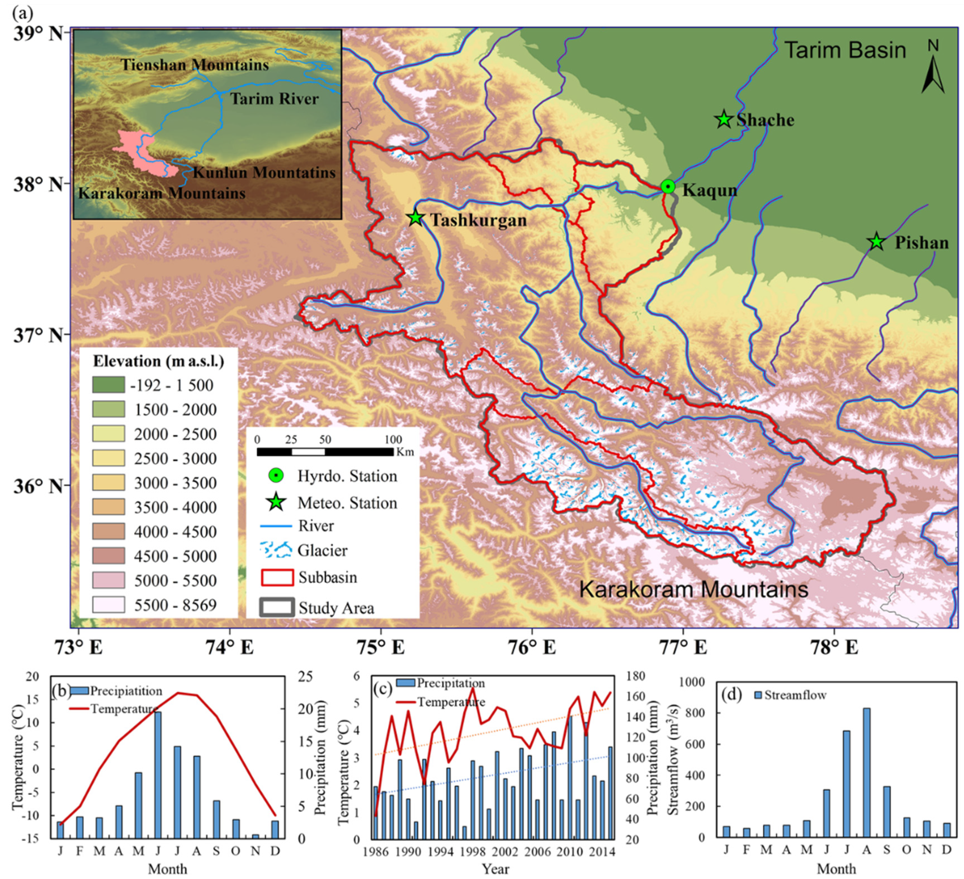
Figure 1. (a) Location of research area; (b) monthly distribution of temperature and precipitation in the Yarkant River basin from 1986 to 2014; (c) annual variations in temperature and precipitation from 1986 to 2015. (d) monthly distribution of streamflow in the Yarkant River basin from 1986 to 2014.
Remotesensing 14 00115 g001
Figure 2. Observed and modeled average discharge with the Yarkant River basin for the calibration period (2005–2010) and the validation periods (1986–2004 and 2011–2014).
Remotesensing 14 00115 g002
Figure 3. Cumulative probabilities of observed (obs), raw, and bias-corrected temperature (a) and precipitation (b) at the Tashkuergan station. Obs, raw and different bias-corrected methods were showed by different type of lines.
Remotesensing 14 00115 g003
Figure 4. Projected annual temperature (a) and precipitation (b) in the Yarkant River from 1986–2100.
Remotesensing 14 00115 g004
Figure 5. Projected monthly average temperature and precipitation for the near-term (a,c) and far term (b,d) during 2015–2100.
Remotesensing 14 00115 g005
Figure 6. Projected annual streamflow (a) in the Yarkant River from 1986 to 2100, and monthly projected streamflow and uncertainties of the Yarkant River during the near term and far term under the SSP126 (b), SSP245 (c), and SSP370 (d) scenarios.
Remotesensing 14 00115 g006
Figure 7. Inter-annual streamflow during the near and far terms under the SSP126 (a), SSP245 (b), and SSP370 (c) scenarios.
Remotesensing 14 00115 g007
Figure 8. Change and uncertainties in projected streamflow components for the Yarkant River during the near term (a) and far term (b) under the SSP126, SSP245, SSP370 scenarios.
Remotesensing 14 00115 g008
Figure 9. Low flow (Q5) and high flow (Q95) in JJA (a,b) and MAM (c,d) in the Yarkant River during the historical period, and near future and far future under the SSP126, SSP245, and SSP370 scenarios.
Remotesensing 14 00115 g009
Figure 10. Cumulative distribution functions (CDFs) for consecutive days below Q5 in JJA and MAM under three SSPs (ac,gi), CDFs for consecutive days above Q95 in JJA and MAM under three SSPs (df,jl).
Remotesensing 14 00115 g010
Table 1. Summary of selected CMIP6 models used in this study.
IDModel NameCountryInstitutionResolution
1BCC-CSM2ChinaBeijing Climate Center100 km
2CNRM-CM6-1FranceCentre National de Recherches Météorologiques100 km
3CNRM-ESM2-1FranceCentre National de Recherches Météorologiques250 km
4GFDL-ESM4AmericaGeophysical Fluid Dynamics Laboratory250 km
5MPI-ESM1-2-HRGermanyMax Planck Institute for Meteorology100 km
6MRI-ESM2-0JapanMeteorological Research Institute100 km
Table 2. Bias-correction methods for GCM-simulated temperature and precipitation.
Bias Correction for TemperatureBias Correction for Precipitation
Linear scaling (LS)Power transformation (PT)
Distribution mapping for temperature using Gaussian distribution (DM)Local intensity scaling (LOCI)
Distribution mapping for precipitation using gamma distribution (DM)
Table 3. Assessment of simulation results of the HEC-HMS model during the calibration and validation periods.
Time PeriodsNSEPBIAS (%)R2
Calibration period (2005–2010)0.805.860.81
Validation period (1986–2004)0.7216.560.70
Validation period (2011–2014)0.839.740.85
Table 4. Frequency-based statistics and time-series-based metrics of daily observed (obs), raw GCMs-simulated (raw) and bias-corrected temperature at the Tashkuergan station.
CMIP6 Models Frequency-Based StatisticsTime-Series-Based Metrics
Mean (°C)Median (°C)Standard Deviation (°C)10th Percentile (°C)99th Percentile (°C)R2RMSEMAE
BCCObs3.985.6010.60−10.7716.70
Raw4.844.2110.43−18.9618.600.8410.629.28
LS3.985.8510.72−11.3716.730.875.544.22
DM3.985.7710.60−11.1316.470.875.384.01
NERM-CM6-1Obs3.985.6010.60−10.7716.70
Raw2.931.456.85−12.2514.550.5111.589.86
LS3.986.0610.99−11.2516.410.826.514.79
DM3.985.4310.60−10.5316.620.855.804.34
CNRM-ESM2-1Obs3.985.6010.60−10.7716.70
Raw1.150.356.44−9.5516.550.5110.498.78
LS3.985.6610.69−10.8016.510.855.834.31
DM3.985.4510.60−10.3416.620.865.624.20
GFDL-ESM4Obs3.985.6010.60−10.7716.70
Raw7.123.8511.06−20.9511.450.4715.7612.53
LS3.986.5313.35−12.9616.120.689.865.51
DM3.985.5710.60−10.0716.110.865.624.16
MPI-ESM1-2-HRObs3.985.6010.60−10.7716.70
Raw4.002.256.92−13.1513.050.5312.1010.39
LS3.986.2911.05−11.3516.320.826.454.64
DM3.985.4710.60−10.3516.700.865.624.19
MRI-ESM2-0Obs3.985.6010.60−10.7716.70
Raw3.410.858.25−15.5514.250.5212.0110.15
LS3.986.6911.56−11.5616.080.816.894.99
DM3.985.5710.60−9.8916.320.875.334.04
Table 5. Frequency-based statistics and time-series-based metrics of daily observed (obs), raw GCMs-simulated (raw) and bias-corrected precipitation at the Tashkuergan station.
CMIP6 Models Frequency-Based StatisticsTime-Series-Based Metrics
Mean (mm)Median (mm)Standard Deviation (mm)10th Percentile (mm)Fre-Quency of Wet Days (%)Intensity of Wet Days (mm)RMSEMAE
BCCObs0.230.001.120.200.051.17
Raw1.520.532.504.240.393.543.00 1.59
PT0.230.001.090.390.053.251.530.41
LOCI0.230.000.761.040.102.081.32 0.41
DM0.110.000.570.220.032.471.24 0.31
CNRM-CM6-1Obs0.230.001.120.200.051.17
Raw1.520.532.194.240.403.142.80 1.60
PT0.230.011.130.300.053.731.59 0.42
LOCI0.200.000.670.920.091.941.31 0.40
DM0.210.001.290.170.044.111.71 0.42
CNRM-ESM2-1Obs0.230.001.120.200.051.17
Raw1.600.802.383.900.423.282.98 1.69
PT0.230.011.150.290.053.731.59 0.42
LOCI0.190.000.700.870.092.081.32 0.40
DM0.230.001.540.130.044.801.90 0.44
GFDL-ESM4Obs0.230.001.120.200.051.17
Raw1.350.701.943.300.353.042.51 1.44
PT0.230.011.190.300.054.611.60 0.41
LOCI0.230.000.680.960.101.921.30 0.40
DM0.200.001.350.140.044.131.74 0.41
MPI-ESM1-2-HRObs0.230.001.120.200.051.17
Raw1.510.702.193.700.403.142.80 1.60
PT0.230.011.130.300.053.651.58 0.42
LOCI0.230.000.670.920.091.941.31 0.40
DM0.210.001.290.170.044.111.71 0.42
MRI-ESM2-0Obs0.230.001.120.200.051.17
Raw1.590.802.193.800.423.122.82 1.67
PT0.230.011.170.300.053.651.58 0.42
LOCI0.170.000.670.900.091.951.29 0.40
DM0.230.001.650.120.044.991.96 0.44
Table 6. Projected changes in mean temperature, total precipitation, mm (%) and streamflow under future scenarios of SSP126, SSP245 and SSP370 during the near term (2021–2049) and far term (2071–2099) compared with the historic period (1986–2014).
VariablesSSPsNear Term (2021–2049)Far Term (2071–2099)
Temperature (°C)SSP1261.723.76
SSP2451.794.29
SSP3701.756.22
Precipitation (mm (%))SSP1269.90 (11.95)11.52 (14.82)
SSP2459.94 (12.00)13.33 (16.09)
SSP3708.95 (10.79)24.09 (29.07)
Streamflow (%)SSP12619.2036.69
SSP24510.6246.11
SSP37014.0170.40
Publisher’s Note: MDPI stays neutral with regard to jurisdictional claims in published maps and institutional affiliations.