Abstract
Recently, remotely sensed data obtained via laser technology has gained great importance due to its wide use in several fields, especially in 3D urban modeling. In fact, 3D city models in urban environments are efficiently employed in many fields, such as military operations, emergency management, building and height mapping, cadastral data upgrading, monitoring of changes as well as virtual reality. These applications are essentially composed of models of structures, urban elements, ground surface and vegetation. This paper presents a workflow for modeling the structure of buildings by using laser-scanned data (LiDAR) and multi-spectral images in order to develop a 3D web service for a smart city concept. Optical vertical photography is generally utilized to extract building class, while LiDAR data is used as a source of information to create the structure of the 3D building. The building reconstruction process presented in this study can be divided into four main stages: building LiDAR points extraction, piecewise horizontal roof clustering, boundaries extraction and 3D geometric modeling. Finally, an architecture for a 3D smart service based on the CityGML interchange format is proposed.
1. Introduction
Nowadays, urban cities are drastically affected by population growth. To solve this problem, urban planning and management relying on remote sensing and geographical information system (GIS) for the sustainable growth of urban areas should be implemented. The new technologies and methods used to gather geographic information have opened new perspectives for urban management and have provided new and dynamic decision-making tools. Besides, with the advanced scanning systems, the captured data and their spatial resolution are becoming significant and precise. The development of an airborne laser, which is a key technology used to extract information about physical surfaces, has resulted in the widespread use of data on buildings and infrastructure at massive and precise scales. Among the applied technologies, we may mention light detection and ranging (LiDAR) which is an active remote sensing system that uses a laser and produces spatially formed point cloud data. Indeed, point clouds are large sets of 3D points defined by their (x, y, z) coordinates. Therefore, urban modeling represents a building by means of a set of planes and straight lines. The former are facades or roofs, while the latter represent their edges. As manual or semi-automatic 3D building reconstructions are time-consuming and difficult, it becomes more challenging to create 3D building models rapidly and easily. Thus, during the last decade, the automatic 3D reconstruction of structures from airborne data has been intensively utilized in photogrammetry, computer graphics and remote sensing industries [1,2].
One of the most used rooftop modeling techniques is the data-driven polyhedral method which is applied to create building models with both complex and simple roof topologies [1]. These data-driven methods are based on a bottom-up approach. This approach starts by extracting primitives such as spheres, cones, planes and cylinders. Then, the basic topology in 3D is evaluated. The last stage consists in grouping and extracting primitives in order to generate urban models. From the aforementioned ideas, we may deduce that the topological consistency maintenance becomes the new challenge of data-driven rooftop reconstruction. Otherwise, piecewise horizontal roofs [3], which is the most common building type in developing countries (e.g., Tunisia), have not been intensively dealt with in the literature.
As shown in Figure 1, the main contributions of the present research work are listed below:
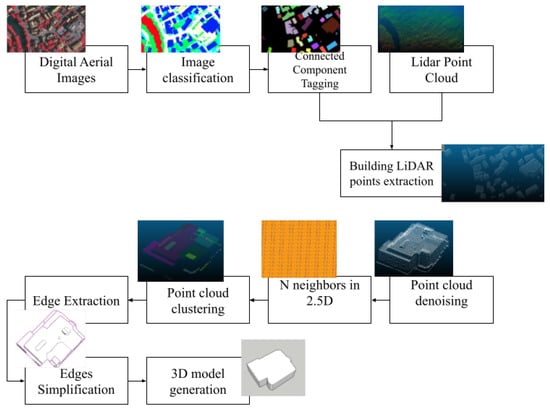
Figure 1.
Pipeline of 3D building reconstruction.
- Exploiting the structure of the point cloud and segmenting the building by utilizing a graph cut-pursuit algorithm coupled with Delaunay triangulation for the adjacency graph.
- Processing these stages in 2.5D to reduce the complexity and the processing time.
- Extracting roof boundaries by using the Delaunay triangulation and the regularized point cloud.
- Generating the 3D model by applying a simple modeling approach that connects all roof levels to the ground through the addition of vertical walls.
- Exporting the extracted 3D model to a CityGML exchange format to ensure the interaction with the 3D representation on a smart city 3D web service.
The techniques of 3D building reconstruction presented in the literature can be classified into two types: parametric modeling and non-parametric modeling. The former begins from a catalog/library of primary buildings and is inspired by predefined models [4,5]. In this catalog, each building model is described by a set of parameters. Thus, to reconstruct a building, it is necessary to know the basic model that resembles it the most. Then, the values that are most likely to be assigned to the parameters of the chosen model are calculated. The fundamental advantage of the parametric modeling of a building is to provide geometric models without visible deformations. However, this method offers only a limited number of building models. On the other hand, non-parametric or associative techniques focus on modeling a building without dividing it into simple parametric blocks [6,7,8]. These techniques analyze the point cloud without making it correspond to a set of parameters. Such modeling is based on a series of operations that are executed to generate an indeterminate form of model. Although it allows for modeling a building regardless of its form, it may produce distorted models.
As we can see, the parametric method is the simplest and the fastest. However, it is limited to treating simple buildings by their geometry. This simple building is linked to a predefined parametric model in the library; the parameters only have to be defined to create the model for it. The second type of model solves the case of any building by suggesting a series of operations that lead to the calculation of a 3D model of a building. Despite the possible risks of collecting distorted models, this type remains the only method that solves the general case of a building, no matter what its shape is.
Concerning the 3D web solutions, ref. [9] presented CityGML as a model for energy diagnosis and support of urban energy policies that introduce three application problems: noise mapping, photovoltaic potential and the calculation of heating needs. Moreover, in [10], the authors developed and deployed a platform to store, analyze and visualize 3D city models via the web. This approach is based on two different technologies for 3D visualization. The first is the NASA WorldWind software development kit (SDK) and the second is the Cesium virtual globe. In [11], the same authors integrated open source technologies and existing services developed by the partners (Open Geospatial Consortium (OGC) CityGML). I-Scope (interoperable Smart City Services through an Open Platform for Urban Ecosystems) offers a routing service for the elderly, a service to evaluate the potential of solar energy at the building level in order to optimize energy consumption and a real-time noise mapping service for environmental monitoring [12].
2. Materials and Methods
In this section, we describe the data utilized in this study and the proposed workflow of the automatic segmentation approach and processing airborne LiDAR point cloud data used in 3D reconstruction and building modeling.
2.1. Materials
The introduced method was supposed to be validated on a laser-scanned point cloud collected in Tunisia. Unfortunately, because of financial issues, collecting the point cloud could not be carried out. The particularity of the buildings in Tunisia is that almost 98% of them have a piecewise horizontal roof shape. Thus, and due to the lack of LiDAR data in Tunisia, the developed technique was validated with the ISPRS benchmark on urban object classification and 3D building reconstruction data collected from the city of Vaihingen [13]. We selected a few specific buildings that validate our criteria (only piecewise horizontal roofs).
2.1.1. LiDAR Dataset
The Vaihingen experiment dataset consists of ten ALS strips taken by Leica Geosystems on 21 August 2008, with a mean flying altitude above ground of 500 m and a 45° field of vision. The median point density is 6.7 points per m and the average strip overlap is 30%. The variation of the point density is significant across the block depending on the overlap, while the average point density in regions covered by only one strip is 4 points per m. The raw data were orthorectified and radiometrically corrected in order to produce an operational point cloud that can be used to generate a group of watertight mesh models that can be used in a variety of applications, including electricity demand estimation, building classification, visibility study, 3D cadastre, navigation visualization and city planning [14].
The LiDAR data is presented as random discrete points with x, y and z values. Characteristics of the dataset are depicted in [15].
2.1.2. Digital Aerial Images
The digital airborne photos are part of the German Society of Photogrammetry, Remote Sensing and Geoinformation (DGPF) test’s high-resolution DMC block. They were taken by RWE Power on 24 July and 6 August 2008, using an Intergraph/ZI DMC [13]. The infrared images that have a radiometric resolution of 11 bits and a ground sampling distance of 8 cm were pan-sharpened. They were stored as 16-bit RGB TIFF files. Two coordinate systems are described in the focal plane (Figure 2).
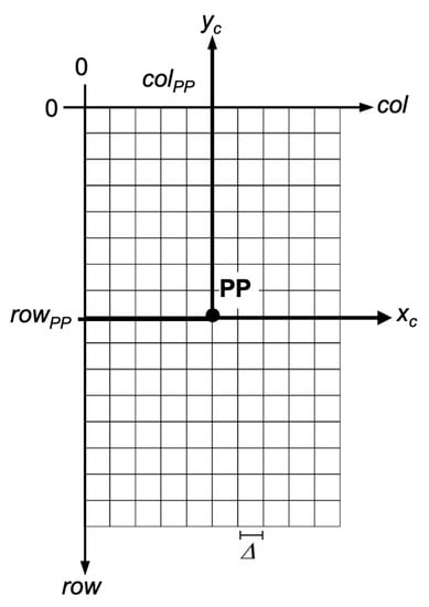
Figure 2.
File and camera coordinate systems.
- File coordinate system (row, col): This system is presented in the image data. Its coordinate axes are parallel to the row and column headings of the aerial image. Its units are pixels, while its root is at the left upper corner of the left upper pixel.
- Camera coordinate system (, ): This system is mathematically positive. Its -axis is parallel to the col axis of the file coordinate system, while its -axis is parallel to its row axis.
The projection center is situated on a straight line that is orthogonal to the focal plane and that crosses the main point. Its distance from the focal plane is the focal range f. The file and camera coordinate systems are described via Equations (1) and (2).
2.1.3. CityGML
CityGML is an official OGC standard that is used to describe, store and exchange 3D city models. The classes of the most important topographic objects in cities and the relations between them are defined by this interchange format. The CityGML model can contain semantic information and relationships between city objects, which is useful for a variety of applications to display buildings information. CityGML is a data interchange model that may be utilized in several geographic web services. One of the most important characteristics of a 3D city model is its level of detail (LoD). It refers to the resemblance of the model to its real-world counterpart and has ramifications for its use [14]. In this paper, we use LiDAR data collected from Berlin, Germany [16]. These data are described below in Table 1.

Table 1.
File information of Berlin CityGML.
2.2. Method
In this study, we propose a workflow to process and create a normalized city model in CityGML based on the XYZ components of the LiDAR point cloud and imagery relying on a graph classification.
Since 98% of the Tunisian buildings have a flat roof, the developed method was applied on piecewise horizontal roofs consisting of flat polygons (of constant height) separated by vertical discontinuities to form vertical rectangles. The process of reconstructing the 3D buildings can be divided into two main stages. The first stage is to re-align the LiDAR and RGB image data to retrieve building LiDAR points from the point cloud. However, the second stage consists of automatically reconstructing the building parts from LiDAR point cloud.
This stage is divided into four sub-steps. First, an adjacency graph was computed to define the neighbors of each 3D point. We opted for 2D adjacency between points using the 2D Delaunay triangulation because our piecewise segmentation relies on a 2.5D analysis. Then, this adjacency graph used the cut-pursuit algorithm [17] to cluster the point cloud into segments of constant components. After clustering the point cloud, the edges of each piecewise constant component of a given building were extracted. Afterwards, the extracted edges were used to generate the 3D envelope of the building.
2.2.1. Connected Component Tagging
Before using connected component tagging, we assume that the multi-spectral aerial images were classified in order to extract the different classes (building, water and trees).
The main objective of this work is to study each building separately. Therefore, each building was extracted individually from the scene. Subsequently, connected component labeling was used to determine the connectivity information extracted from the previously segmented image. This technique allowed for the transition from one analysis level, linked to the pixel scale, to another level, related to the information about the different regions of the image.
This stage (Figure 3) was performed using a grassfire [18] algorithm applied to calculate the distance between a given pixel and the edge of a region. This phase can be described as “firing” the boundaries of an image region to produce descriptors such as the backbone or midline of the region. Only the building class is extracted and labeled.

Figure 3.
Connected component labeling: (a): classified image (b) labeled image.
2.2.2. Registration and Extraction of the LiDAR Points of a Building
As LiDAR data and digital aerial images have entirely different spatial resolutions, they cannot be acquired simultaneously. To resolve this problem, we need to recalibrate the data to be represented in the same geographic grid [19] by merging these two types of data to extract the class of buildings from the point cloud.
A world file was utilized to perform an image-world transformation that allowed converting the coordinates of the image into real-world coordinates. This file contains the following lines:
- Line 1 (A): x-direction pixel dimension.
- Line 2 (D): rotation around the y-axis.
- Line 3 (B): rotation around the x-axis.
- Line 4 (E): y-direction pixel dimension (usually negative).
- Line 5 (C): x-coordinate of the upper-left pixel midpoint.
- Line 6 (F): y-coordinate of the upper-left pixel middle.
The algorithm of building point cloud extraction is described below Algorithm 1:
| Algorithm 1: Extract building LiDAR point cloud |
| Input: the input file name is the same used as given in the benchmark of the ISPR [13]. |
 |
Where
- mg.rows: height of the image.
- xPixel and yPixel are the coordinate of the projection of the point cloud (xCloud, yCould, zCloud) on the classified RGB image.
The previous algorithm can also produce a non-classified LiDAR point cloud. The equivalent of the labeled RGB image can be extracted as shown in Figure 4.
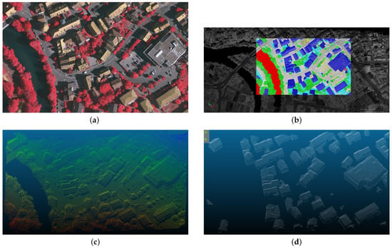
Figure 4.
(a) Top mosaic RGB image, (b) LiDAR and matched image, (c) point cloud of the top mosaic RGB, and (d) buildings LiDAR point cloud.
2.3. Point Cloud Denoising
The point cloud information provided by sensor scans generally has different densities. Furthermore, measurement errors result in sparse outliers that further distort the results. Echoes from walls and vertical surfaces may be present in the LiDAR point cloud. In 2.5 dimension, multiple superposed points will produce noise in the data and complicate the local point cloud feature estimation, such as curvature changes or surface normals, thus resulting in incorrect values and possibly creating point cloud clustering failures.
To solve this problem, data must be preprocessed to remove the noisy point cloud from the scene. In this study, noisy points are vertical points. A statistical outlier removal filter (SOR) [20] was employed in this stage to filter outlier data.
A statistical study was, next, conducted in order to remove the imperfections. Subsequently, point surroundings that do not meet specific criteria were omitted. The distance distribution between a point and its neighbors was used to accomplish sparse outlier reduction. After that, the average distance between a specific point and its neighbors was calculated. After obtaining a Gaussian distribution, endpoints, whose mean distances were outside an interval defined by standard deviation and the global distances mean, were clipped. The endpoints were considered outliers (Figure 5).
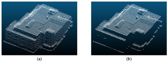
Figure 5.
SOR result: (a) Noisy Point Clouds, (b) Filtered point cloud.
2.3.1. N Neighbors in 2.5D
The spatial structure of a point cloud can be represented by a non-oriented graph G = (V, E) (Figure 6) where each node represents a point in the cloud, and where the edges encode their adjacency relation. It is important to note that this adjacency graph is not the same as the neighborhood graph used to calculate the local geometric features.
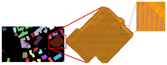
Figure 6.
Adjacency graph using the Delaunay triangulation.
In this section, we present the adjacency graph that captures the spatial structure of a point cloud. In the performed experiments, each building was extracted separately. For each point in the point cloud, two vectors (source and target) were calculated. The source vector contains all of the point cloud, while the target vector includes the neighbors of each point of the source vector. This spatial relation was obtained by a Delaunay triangulation. Later, this step would be applied as input to the cut-pursuit clustering algorithm.
2.3.2. Point Cloud Clustering Using Cut-Pursuit Algorithm
Let V be a set of point clouds acquired by an aerial LiDAR in an urban scene. Our objective is to obtain a piecewise horizontal segmentation of V. The cut-pursuit [17] algorithm was used to perform this segmentation. In fact, cut pursuit segments a weighted graph G = (V, E, w) with values on its nodes and weights on its edges by minimizing the variance of the values inside the clusters and the sum of weights of the cut edges (between clusters). As piecewise horizontal segmentation is the focus of this research work, the values on the nodes are the Z coordinates of each point. The chosen adjacency is the 2D Delaunay triangulation, and the edge weight is given by:
As shown in Figure 7, the cut-pursuit algorithm [17] takes as input a non-oriented graph (Figure 7a) representing the neighbor’s relations and producing a segmentation of this graph in clusters according to the Z value of each point. The vertices of the graph G were originally coupled into a single segment. This graph was recursively cut into constantly connected segments. At each iteration (from (a) to (e)), a reduced graph (g) encoding the adjacency between constant segments was calculated. Then, the values associated with each constant segment were computed using the smallest reduced graph. The vertex colors denote their values, from low (in green) to high (in yellow).

Figure 7.
Graph regularization according to the Z value: a reduced graph (g) is calculated at each iteration from (a–e), encoding the adjacency between constant segments.
In the application process of our method, each building was treated separately. As the present study deals with piecewise horizontal roofs, we chose a building that verifies the constraint shown in Figure 8a. At this level, the point cloud was clustered into piecewise constant components according to the Z value of all points, as demonstrated in Figure 8b. The next stage consists of detecting the contour of each component.
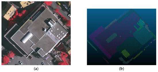
Figure 8.
Clustering result obtained using the cut-pursuit algorithm: (a) real building image, (b) building clustered points.
2.3.3. Edge Extraction
In order to get a 3D model consisting of flat planar polygons separated by vertical surfaces, a 2D vector was segmented into adjacent polygons sharing common borders. Our main objective is to use the Delaunay triangulation to create these edges in a topologically consistent way by generating polygonal boundary lines separating each cluster (Figure 9). A given building may have two types of edges: internal boundaries (shared by components) and external boundaries.
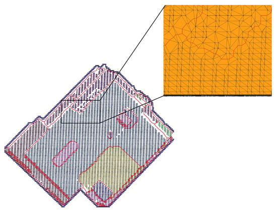
Figure 9.
Extracted edges matched with Delaunay triangulation and regularized point cloud in 2.5D.
Internal Boundaries
In order to generate the polygonal boundary lines, the triangles of the Delaunay triangulation were divided into three sets based on the cluster labels of their three vertices as follows:
- Delaunay triangle has three different labels (Figure 10a). Triangle vertices were distinctly labeled, which means that each vertex belongs to a specific cluster. These triangles were split between the three clusters by dividing the triangle along the three edges linking the barycenter of the triangle to the middles of its edges, as revealed in Figure 10a.
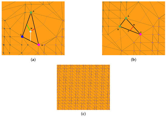 Figure 10. The three types of triangles: (a) triangles with 3 distinct labels, (b) triangles with 2 mixed labels, and (c) triangles with 3 identical labels.
 - Delaunay triangle has two different labels (Figure 10b). The two vertices A and B of the triangle have the same label, and the third vertex C has a different label. These triangles were split between two clusters by cutting the triangle along the edge between the middles of and , as exposed in Figure 10b.
- Same labeled points (Figure 10c). The three vertices of the triangle have the same label, indicating that they belong to the same cluster. The triangle lays completely in a single cluster.
External Boundaries: Building Footprint
The previous section explained how the edges between the components of the roof were extracted. Similarly, in this section, we show how the roof’s external edges, which form the building footprint, were extracted. Since only the points belonging to a single building were considered in the experiments, no points existed outside the footprint to define these external edges, as previously demonstrated in triangle splitting. This issue is solved by keeping the LiDAR points outside the building in a bounding box of its points and giving them a specific unused label. After that, the above explained procedure generated these external edges.
All the split edges were inserted in a planar arrangement using the Computational Geometry Algorithms Library (CGAL) Library [21]. Each cell of this arrangement is either a polygon or the infinite face, which ensures that the result of this stage is a polygonal decomposition of the 2D plane with a well-defined cell topology (adjacent polygons share exactly one or multiple edges).
2.3.4. Edges Simplification
Obviously, the detected boundaries are not smooth. Even if they are polygonal, they are much more complex than the polygonal structure of the roof. Since the borders of nearby planar roof areas are not strictly aligned together in practice due to residual sensor noise, these contours are presented in a simpler manner using the Douglas–Peucker algorithm which is [22] applied to simplify a polyline (set of nodes) by only keeping a subset of its vertices. The algorithm works in a top-down manner by recursively splitting a polyline, approximating the original polyline until the approximation error becomes inferior to a certain threshold. In this study, it is applied to each polyline linking two triple points (barycenter of a fully split triangle) (Figure 10a). The Douglas–Peucker is used to smooth these edges, as shown in Figure 11b.
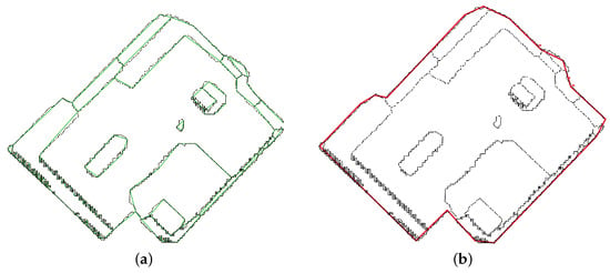
Figure 11.
(a) Smoothed boundaries in green –– and non-smoothed boundaries in black - - -, (b) Building footprint in red ––.
At each stage, one pointer traverses all the nodes between the terminals, and the other pointer selects the node furthest from the segment formed by the terminals:
- If there is no node between the limits, the algorithm ends.
- If this distance is smaller than a defined threshold, it means that all the nodes are between the terminals.
- If it is greater than the threshold, the polyline cannot be directly simplified. In this case, we apply the algorithm recursively on two sub-parts of the polyline: from the first terminal to the remote node and from the remote node to the final terminal.
2.3.5. 3D Model Generation
In this stage, the building point cloud was divided into many planar roof components, each of which has its own set of boundaries. Each boundary was treated as a roof polygon in a simple modeling approach, and it was connected to the ground by adding vertical walls. By applying this method, solid building blocks were formed. Then, they were combined to construct 3D building models. In fact, a 2.5D building model was constructed by combining planar roof patches with vertical facades. As the main hypothesis was to handle only piecewise horizontal roofs, we selected this building to validate our approach. Regarding buildings with a non-flat roof, a simple reconstruction was performed by extruding the outer edge, extracted by performing the stage mentioned above, with a height equal to its maximum Z value. Figure 12 illustrates the extracted buildings in 3D, while Figure 13 shows the 3D buildings that were added to OpenStreetMap (OSM).
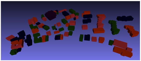
Figure 12.
Generated 3D buildings.
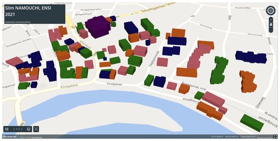
Figure 13.
3D building displayed on OSM.
2.3.6. LoD1 3D CityGML Building Model Generation
In order to validate our approach on a large 3D building scene, which cannot be achieved because our 3D modeling approach deals only with a specific type of building, for a piecewise roof we used a CityGML representation from the city of Berlin. The main stages of converting a CityGML file into a visual 3D model on the web browser are listed below (see Figure 14):
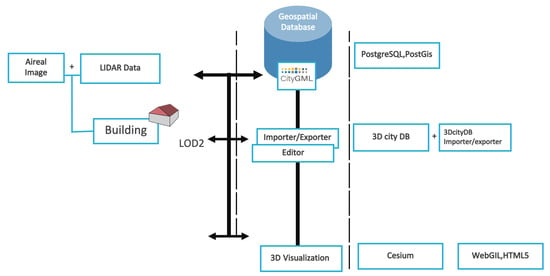
Figure 14.
General architecture for 3D smart web services.
On the other hand, in order to manage the elements of the database, 3D City DB and the 3D City DB Importer/Exporter were employed. Thanks to Cesium, the geospatial engine, displaying the 3D building models based on HTML5 and Web GL is allowed.
3. Results
In this section, we present the results obtained by the proposed approach. First, a confusion matrix was calculated to evaluate the performance of the LiDAR buildings point cloud extraction phase. Then, the mean root mean square error (RMSE) and the standard deviation were utilized in order to determine the geometrical accuracy of the roof polygons and obtain the final reconstructed building.
3.1. Building LiDAR Point Cloud Extraction Evaluation
In order to calculate the precision of the extraction, it is necessary to compute the difference between the edges of the building according to the cloud of points and the detected edges. Therefore, the difference between the actual building contour and the detected building contour combines the precision of laser scanning and the precision of extraction. Since our objective is to estimate the precision of the developed automatic extraction method, the reference image was obtained by manual digitization of the point cloud by using the CloudCompare software [23].
To quantify the differences between the resulting image and the reference image, we applied the estimation method proposed by [24]. This technique is based on the calculation of a confusion matrix in which the result and the reference are compared (see Table 2). At the end of processing, we obtained two classes: the “buildings” class and the “non-buildings” class.

Table 2.
Confusion matrix used to calculate the overall precision of the building extraction.
The confusion matrix in Table 2 contains the following values:
- a: the number of pixels representing the well-classified buildings.
- b: the number of pixels representing the buildings classified in the calculated mask.
- c: the number of pixels of the non-building class that are misclassified.
- d: the number of pixels of the non-buildings class which are classified in the two images of the same way.
- e: the total number of the pixels tested.
Based on the above presented classification, three types of errors are obtained:
- Type I error: is equal to and represents the proportion of pixels classified as building in the resulting image.
- Type II error: is equal to and represents the proportion of pixels classified as non-building in the resulting image.
- The total error: is equal to and represents the proportion of misclassified pixels in the resulting image. Then, a mark or a mention is attributed to the value taken by these errors. For this reason, the authors in [24], suggested the following qualitative assessments:
- “Bad”: if the total error is greater than 50%.
- “Medium”: if the total error is between 10% and 50%.
- “Good”: if the total error is less than or equal to 10%.
Table 3 collects the errors calculated by the confusion matrix, the errors belonging to type I and type II, with the total error as well as the notation assigned to the result.

Table 3.
Qualitative assessment to the extraction of buildings carried out on the point clouds.
From Table 3, we notice that Type I and Type II errors vary between 1.56% and 2.70%, which means that less than 5% of the pixels were assigned to the wrong class. In addition, the values of Error II are excellent (less than 3%), which demonstrates that the LiDAR building point extraction algorithm applied on the classified image has allowed for separating soil classes and oversoil. From this observation, we may conclude that the pixels of the ground class (that represent the ground, small trees and noise) were detected with very high precision because of the fact that image classification is based on ground truth, as long as the error is justified by the LiDAR point cloud resolution. The better the point cloud resolution is, the better the segmentation will be.
Rather than focusing on the errors, we could also calculate the total precision by and obtain percentages of detection above 95%. Consequently, the precision of the segmentation results obtained on the available point clouds are very satisfactory.
3.2. Geometrical Accuracy of the Obtained Reconstructed Building
From a visual point of view, the obtained results are good. However, it is necessary that a visual validation and a quantitative analysis should be applied together in order to validate this work. The mean of the Euclidean distance (along the and -axes) between the i-th point of each segmentation model and the corresponding nearest neighbor point of the reference dataset is used in Equation (4). See table Table 4 for the RMSE results.

Table 4.
Average performances of the geometry accuracy on the building in Vaihingen (Germany) obtained by the proposed approach in comparison to the reference data.
The CityGML model was efficiently applied on the 3D WebClient toolbox panel (see Figure 15). The level of details (LOD) concept was supported by the 3D Web Client (Cesium [25]), which is a common solution used in 3D computer graphics and GIS for efficient distribution and rendering of heterogeneous data [26]. According to this concept, the data tiles with a higher resolution are loaded and visualized when the observer visualizes them from a short distance.
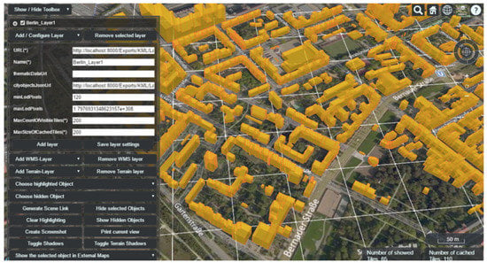
Figure 15.
Untextured building 3D visualization.
4. Discussion
In this paper, we examined a very specific roof type which is the piecewise horizontal roof. A new pipeline for 3D urban modeling using aerial LiDAR data was also proposed. The Delaunay triangulation, cut-pursuit and the Ramer–Douglas–Peucker algorithm were applied to generate a 3D building model. Possible future work lays within two major directions. First, the 3D urban reconstruction method can be enhanced by adding texture in order to create more realistic models. The second future project research consists of integrating a smart city 3D web service to simulate some possible threats in the city and determine their impact on the buildings.
To conclude, it should be noted that the quality of the final result is largely determined by the characteristics of the point cloud (density of points, precision of positioning of the points and presence of noise) and the architectural complexity of the roof.
The following recommendations can be drawn from this work:
- Focusing on isolated buildings can be very interesting. It would be equally interesting to extract each building separately for further processing as it allows for the possibility of displaying the building corresponding to a specific criterion (height, surface, nature, etc.).
- During the denoising stage, some points may be lost. Therefore, choosing the adequate standard deviation multiplier threshold (n Sigma) and the specific number of points to use in mean distance estimation is very important.
- The edge simplification stage also requires a good epsilon () value. In fact, a high () will skip some internal segments and extract only continuous outer boundaries.
Author Contributions
Methodology, software, validation, formal analysis, resources, data, writing— original draft preparation, S.N.; writing—review and editing, S.N. and I.R.F.; supervision, I.R.F. All authors have read and agreed to the published version of the manuscript.
Funding
This research received no external funding.
Institutional Review Board Statement
Not applicable.
Informed Consent Statement
Not applicable.
Data Availability Statement
The data that support the findings of this study are available in the ISPRS benchmark 2012 [13].
Acknowledgments
This project is carried out under the MOBIDOC scheme, funded by the EU through the EMORI program and managed by the ANPR in cooperation with the National Mapping and Remote Sensing Center (CNCT), Ministry of Defense.
Conflicts of Interest
The authors declare no conflict of interest.
References
- Li, L.; Yao, J.; Tu, J.; Liu, X.; Li, Y.; Guo, L. Roof Plane Segmentation from Airborne LiDAR Data Using Hierarchical Clustering and Boundary Relabeling. Remote Sens. 2020, 12, 1363. [Google Scholar] [CrossRef]
- Wang, R. 3D building modeling using images and LiDAR: A review. Int. J. Image Data Fusion 2013, 4, 273–292. [Google Scholar] [CrossRef]
- Namouchi, S.; Vallet, B.; Farah, I.R.; Ismail, H. Piecewise Horizontal 3D Roof Reconstruction from Aerial Lidar. In Proceedings of the IGARSS 2019–2019 IEEE International Geoscience and Remote Sensing Symposium, Yokohama, Japan, 28 July–2 August 2019; pp. 8992–8995. [Google Scholar] [CrossRef]
- Suveg, I.; Vosselman, G. Reconstruction of 3D building models from aerial images and maps. ISPRS J. Photogramm. Remote Sens. 2004, 58, 202–224. [Google Scholar] [CrossRef] [Green Version]
- Jarząbek-Rychard, M.; Borkowski, A. 3D building reconstruction from ALS data using unambiguous decomposition into elementary structures. ISPRS J. Photogramm. Remote Sens. 2016, 118, 1–12. [Google Scholar] [CrossRef]
- Verma, V.; Kumar, R.; Hsu, S. 3D building detection and modeling from aerial LIDAR data. In Proceedings of the 2006 IEEE Computer Society Conference on Computer Vision and Pattern Recognition (CVPR’06), New York, NY, USA, 17–22 June 2006. [Google Scholar]
- Jarzabek-Rychard, M.; Maas, H.G. Aerial image based geometric refinement of building models derived from airborne lidar data. In Proceedings of the GEOBIA 2016: Solutions and Synergies, Enschede, The Netherlands, 14–16 September 2016. [Google Scholar]
- Albeaik, S.; Alrished, M.; Aldawood, S.; Alsubaiee, S.; Alfaris, A. Virtual Cities: 3D Urban Modeling from Low Resolution LiDAR Data. In Proceedings of the 25th ACM SIGSPATIAL International Conference on Advances in Geographic Information Systems, Association for Computing Machinery, New York, NY, USA, 6–9 November 2017. [Google Scholar]
- Nouvel, R.; Schulte, C.; Eicker, U.; Pietruschka, D.; Coors, V. CityGML-based 3D City Model for Energy Diagnostics and Urban Energy Policy Support. In Proceedings of the BS2013: 13th Conference of International Building Performance Simulation Association, Chambéry, France, 26–28 August 2013. [Google Scholar]
- Prandi, F.; Devigili, F.; Soave, M.; Di Staso, U.; De Amicis, R. 3D web visualization of huge CityGML models. ISPRS Int. Arch. Photogramm. Remote Sens. Spat. Inf. Sci. 2015, XL-3/W3, 601–605. [Google Scholar] [CrossRef] [Green Version]
- Prandi, F.; De Amicis, R.; Piffer, S.; Soave, M.; Cadzow, S.; Boix, E.G.; D’Hondt, E. Using citygml to deploy smart-city services for urban ecosystems. Int. Arch. Photogramm. Remote Sens. Spat. Inf. Sci. 2013, 4, W1. [Google Scholar] [CrossRef] [Green Version]
- Singh, S.P.; Jain, K.; Mandla, V.R. Virtual 3d City Modeling: Techniques and Applications. ISPRS Int. Arch. Photogramm. Remote Sens. Spat. Inf. Sci. 2013, XL-2/W2, 73–91. [Google Scholar] [CrossRef] [Green Version]
- ISPRS Test Project on Urban Classification, 3D Building Reconstruction and Semantic Labeling. 2012. Available online: http://www2.isprs.org/commissions/comm3/wg4/tests.html (accessed on 12 September 2018).
- Biljecki, F.; Stoter, J.; Ledoux, H.; Zlatanova, S.; Çöltekin, A. Applications of 3D City Models: State of the Art Review. ISPRS Int. J. Geo-Inf. 2015, 4, 2842–2889. [Google Scholar] [CrossRef] [Green Version]
- ISPRS Test Project on Urban Classification and 3D Building Reconstruction. Available online: https://www2.isprs.org/media/komfssn5/complexscenes_revision_v4.pdf (accessed on 12 February 2019).
- Berlin 3D Building Models in Level of Detail 2 (LoD 2). Available online: Https://fbinter.stadt-berlin.de/fb/index.jsp (accessed on 12 September 2018).
- Landrieu, L.; Obozinski, G. Cut Pursuit: Fast algorithms to learn piecewise constant functions. Artif. Intell. Stat. 2016, 51, 1384–1393. [Google Scholar]
- Blum, H. A Transformation for Extracting New Descriptors of Shape. In Symposium on Models forSpeech and Visual Form; Whaten-Dunn, W., Ed.; MIT Press: Cambridge, MA, USA, 1967. [Google Scholar]
- Megahed, Y.; Shaker, A.; Yan, W.Y. Fusion of Airborne LiDAR Point Clouds and Aerial Images for Heterogeneous Land-Use Urban Mapping. Remote Sens. 2021, 13, 814. [Google Scholar] [CrossRef]
- Rusu, R.B.; Cousins, S. 3D is here: Point Cloud Library (PCL). In Proceedings of the 2011 IEEE International Conference on Robotics and Automation, Shanghai, China, 9–13 May 2011; pp. 1–4. [Google Scholar] [CrossRef] [Green Version]
- The Computational Geometry Algorithms Library (CGAL). 1996. Available online: https://www.cgal.org/ (accessed on 12 November 2018).
- Ramer, U. An iterative procedure for the polygonal approximation of plane curves. Comput. Graph. Image Process. 1972, 1, 244–256. [Google Scholar] [CrossRef]
- Cloud Compare Software for 3D Point Cloud and Triangular Mesh Processing Tool. Available online: http://cloudcompare.org (accessed on 12 November 2018).
- Sithole, G.; Vosselman, G. Report: ISPRS comparison of filters. ISPRS Comm. III Work. Group. 2003. Available online: https://studylib.net/doc/11841668/comparison-of-filtering-algorithms-george-sithole--george... (accessed on 12 June 2021).
- 3D Geospatial Visualization for the Web. Available online: Https://cesium.com/platform/cesiumjs/ (accessed on 12 July 2021).
- Biljecki, F.; Ledoux, H.; Stoter, J. An improved LOD specification for 3D building models. Comput. Environ. Urban 2016, 59, 25–37. [Google Scholar] [CrossRef] [Green Version]
Publisher’s Note: MDPI stays neutral with regard to jurisdictional claims in published maps and institutional affiliations. |
© 2021 by the authors. Licensee MDPI, Basel, Switzerland. This article is an open access article distributed under the terms and conditions of the Creative Commons Attribution (CC BY) license (https://creativecommons.org/licenses/by/4.0/).