
Feature Comparison of Two Mesoscale Eddy Datasets Based on Satellite Altimeter Data


Abstract
:
1. Introduction
2. Data and Methods
2.1. Data
2.1.1. Satellite Remote Sensing Data
2.1.2. Mesoscale Eddy Trajectory Atlas Product Version 2.0 (META v2.0)
2.1.3. Global Ocean Mesoscale Eddy Atmospheric-Oceanic-Biological Interaction Observational Dataset 1.0 (GOMEAD v1.0)
2.2. Eddy Detection Schemes
2.2.1. META Eddy Detection
- The amplitude of the test area must be equal to or smaller than that of the area already defined.
- The distance between the two remotest points must be less than a maximum diameter for a given eddy. Distance max = 700 km for latitudes lower than 25°, or 400 km for latitudes higher than 25°.
- No more than 2000 pixels.
- No latitude holes on the edges and no holes within the interior of the area.
2.2.2. GOMEAD Eddy Detection
- The velocity component u’ in the north–south direction have opposite signs on both sides of the eddy center, and their absolute value increases as they move away from the center.
- The velocity component v’ in the east–west direction have opposite signs on both sides of the eddy center, and their absolute value increases as they move away from the center.
- The minimum velocity point within the selected range is the undetermined eddy center.
- The direction of the two adjacent velocity vectors around the eddy center must be close to each other and must be in the same or adjacent quadrants to ensure the same direction of rotation.
2.2.3. Similarities and Differences of Two Datasets
2.3. Eddy Tracking Method
2.3.1. META Dataset Eddy Tracking Method
2.3.2. GOMEAD Dataset Eddy Tracking Method
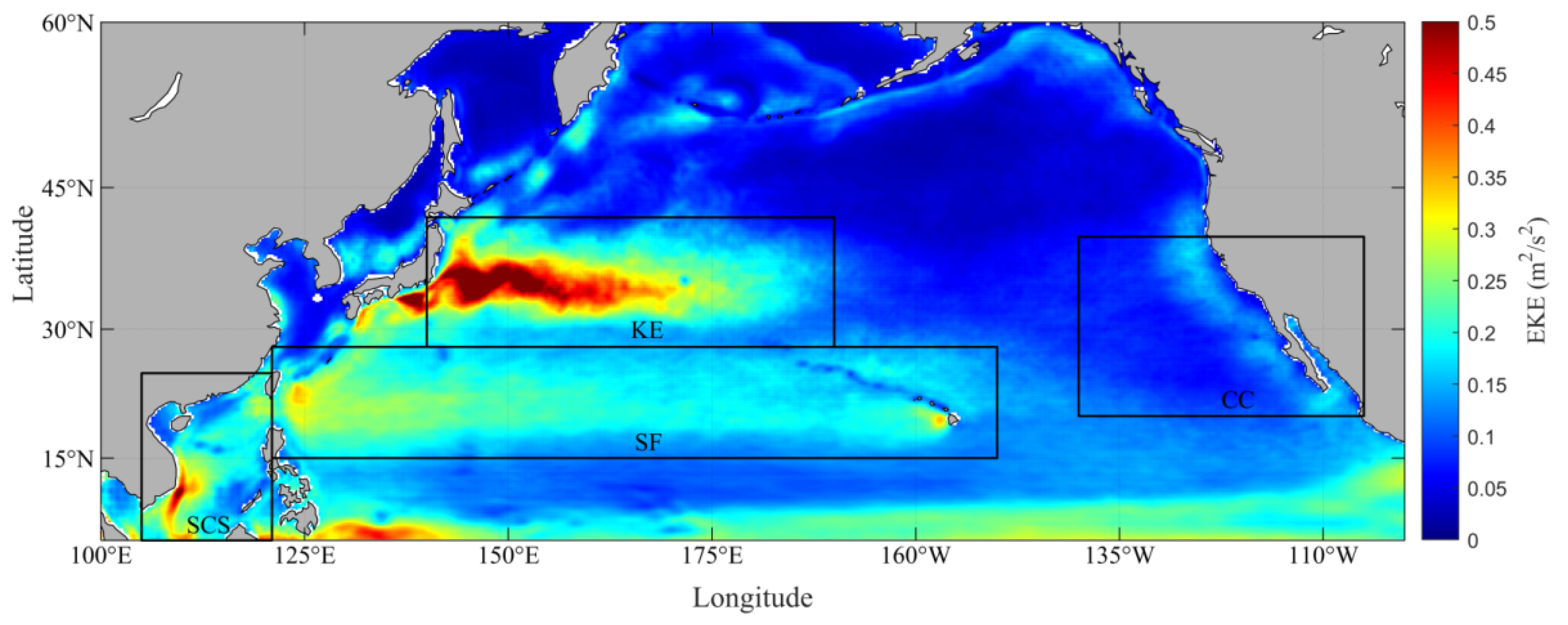
2.4. Introduction to the Study Area
3. Results
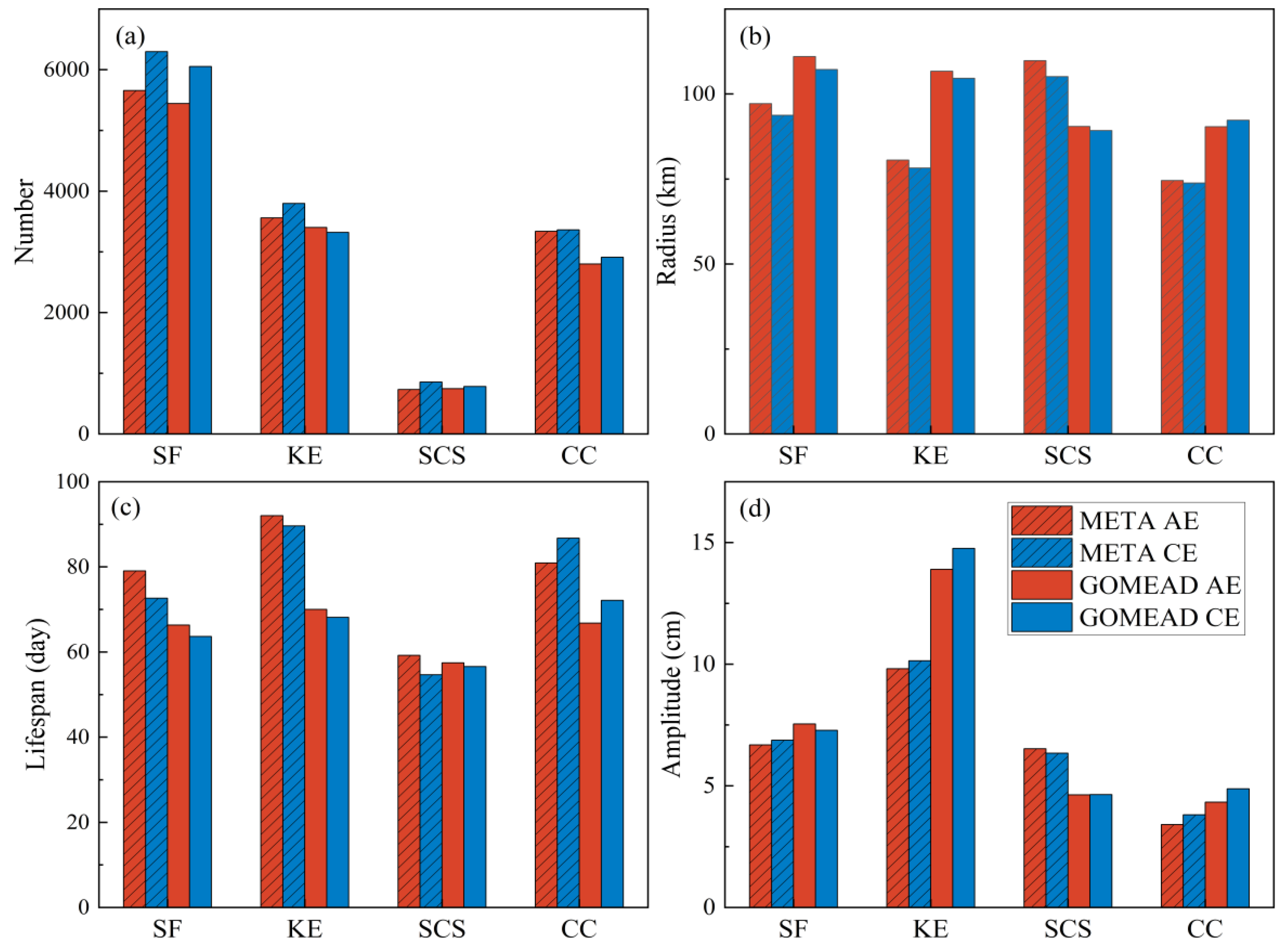
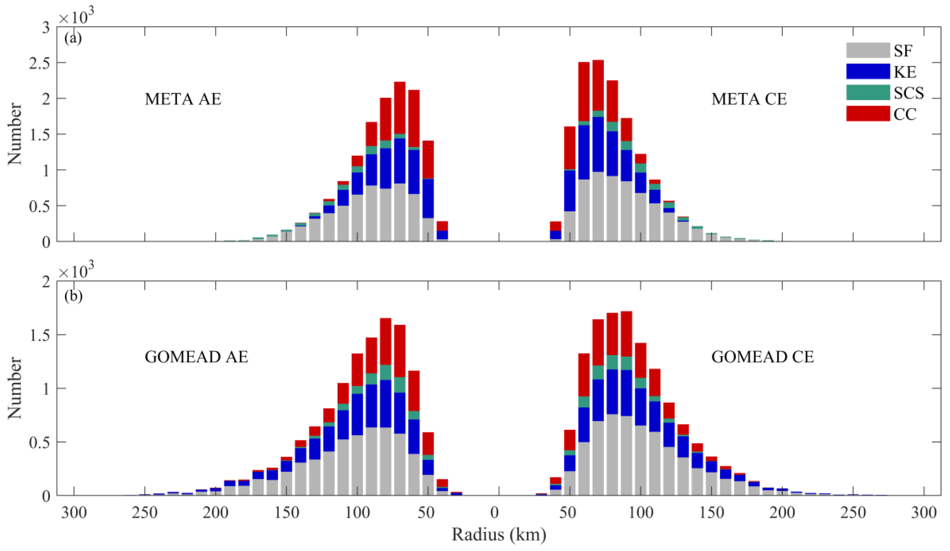
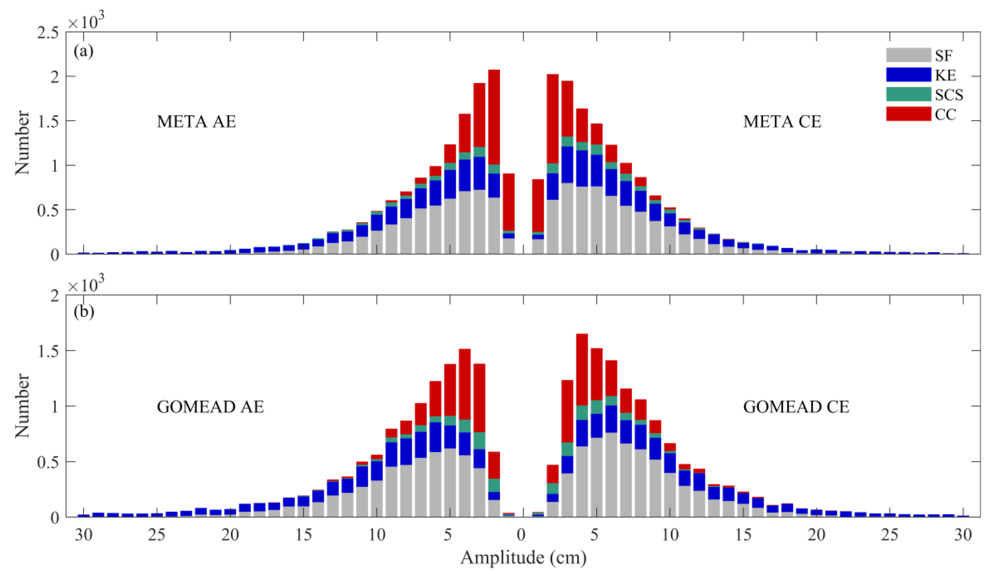
3.1. Eddy Characteristics Statistics
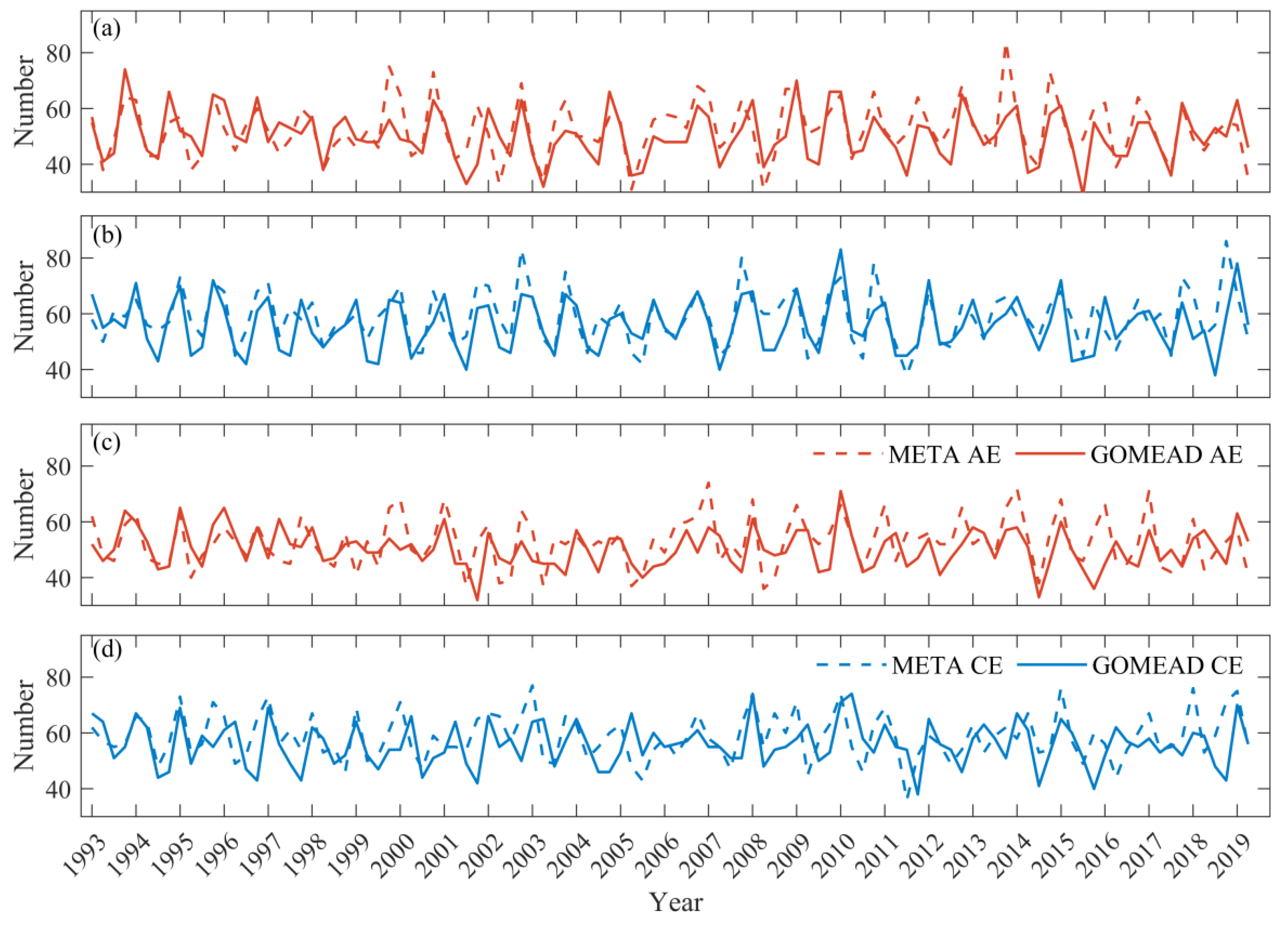
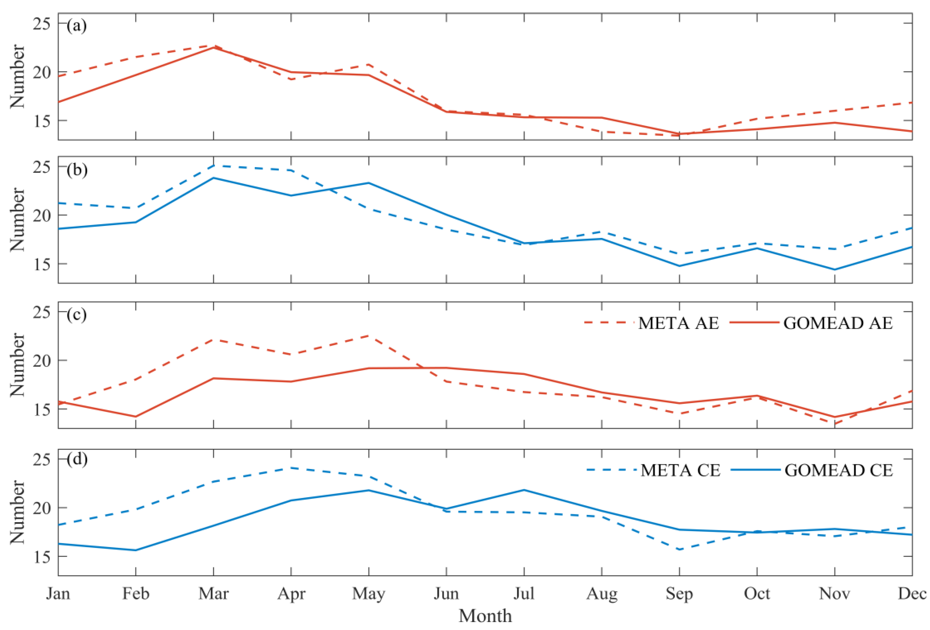
3.2. Temporal Distribution
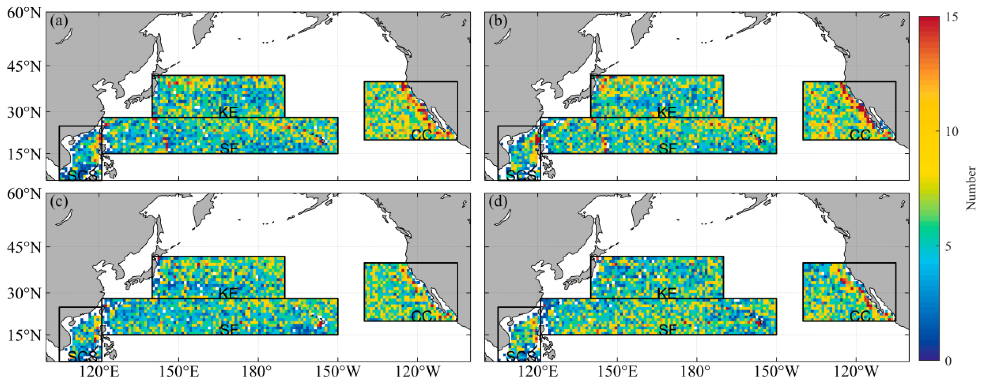
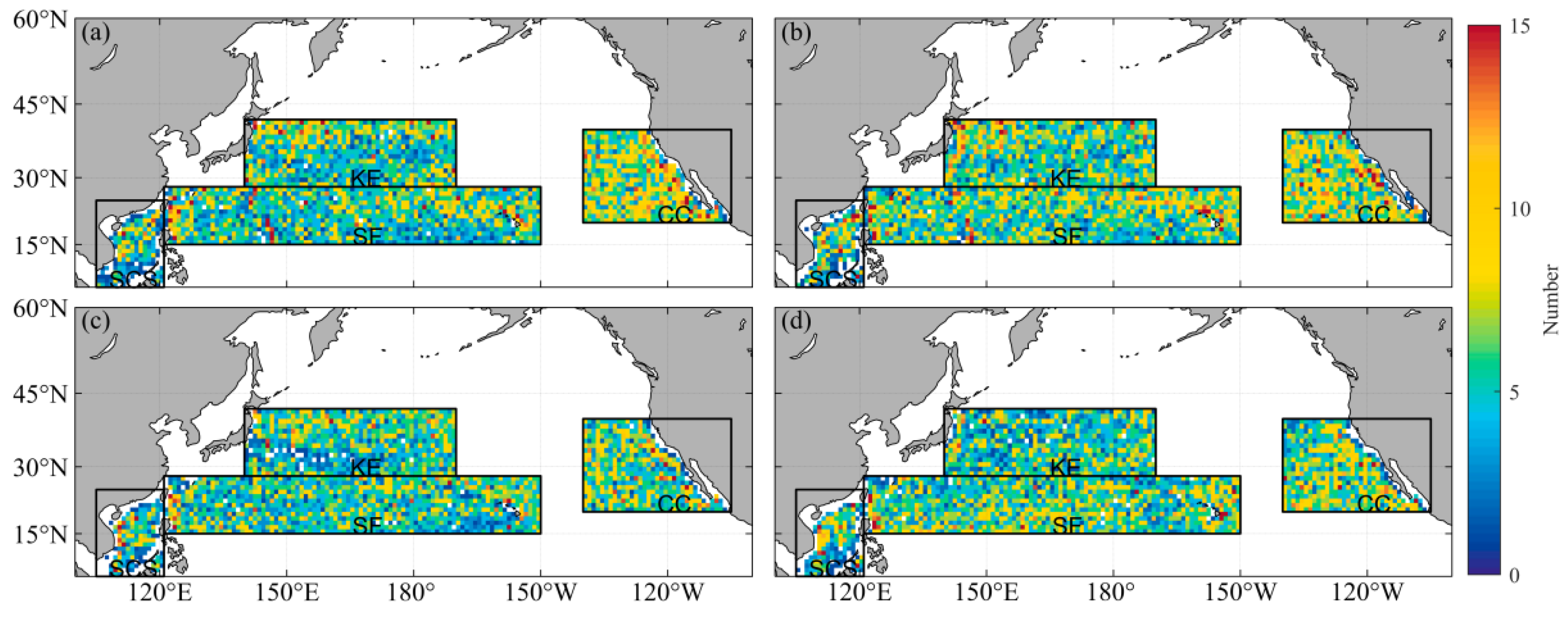
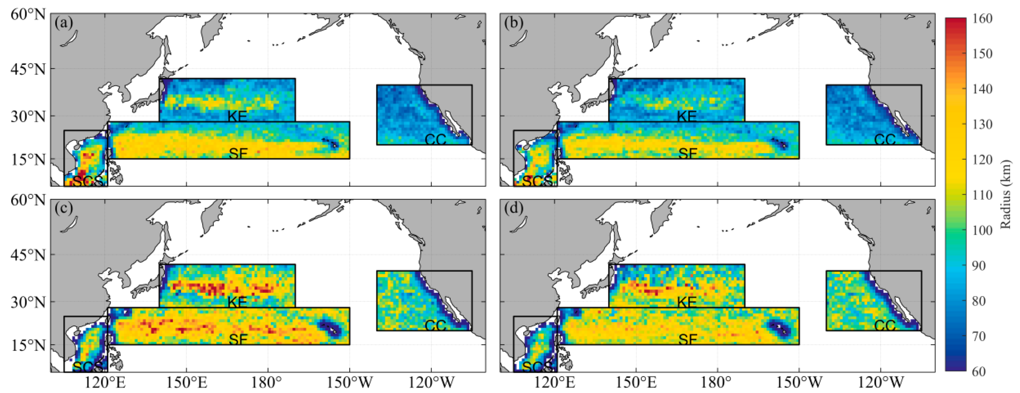
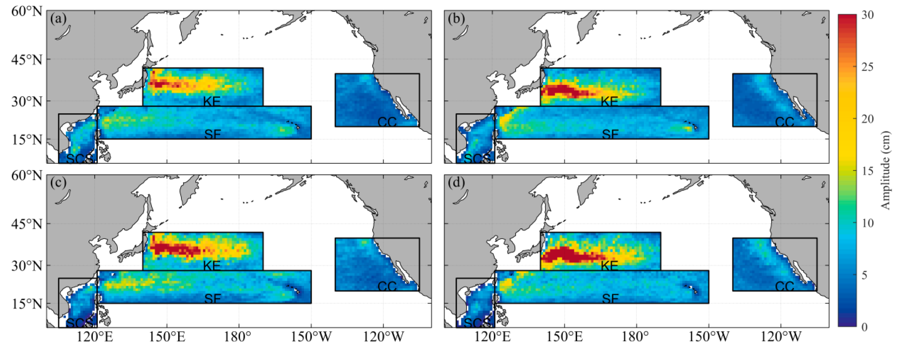
3.3. Spatial Distribution
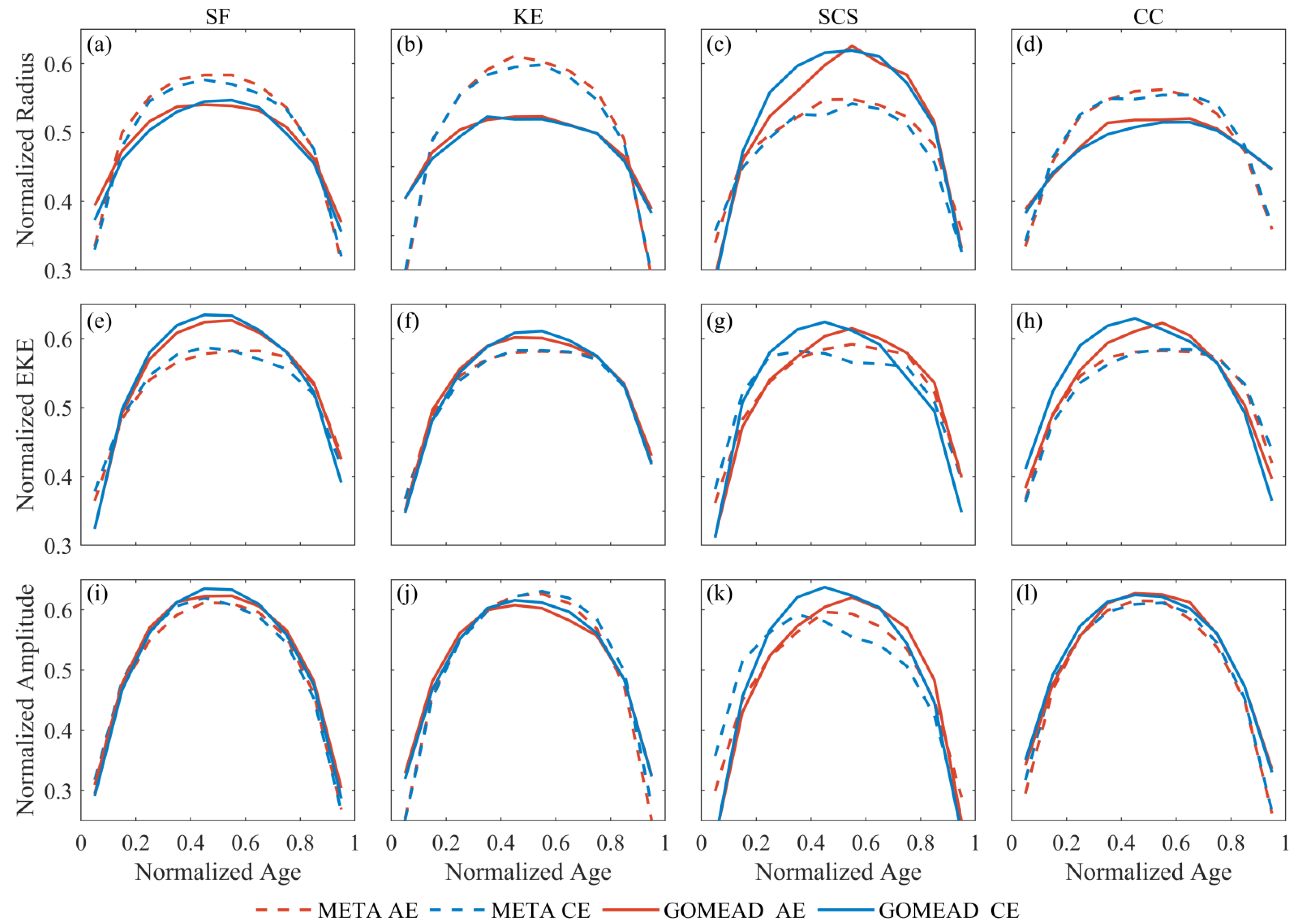
3.4. Time Evolution
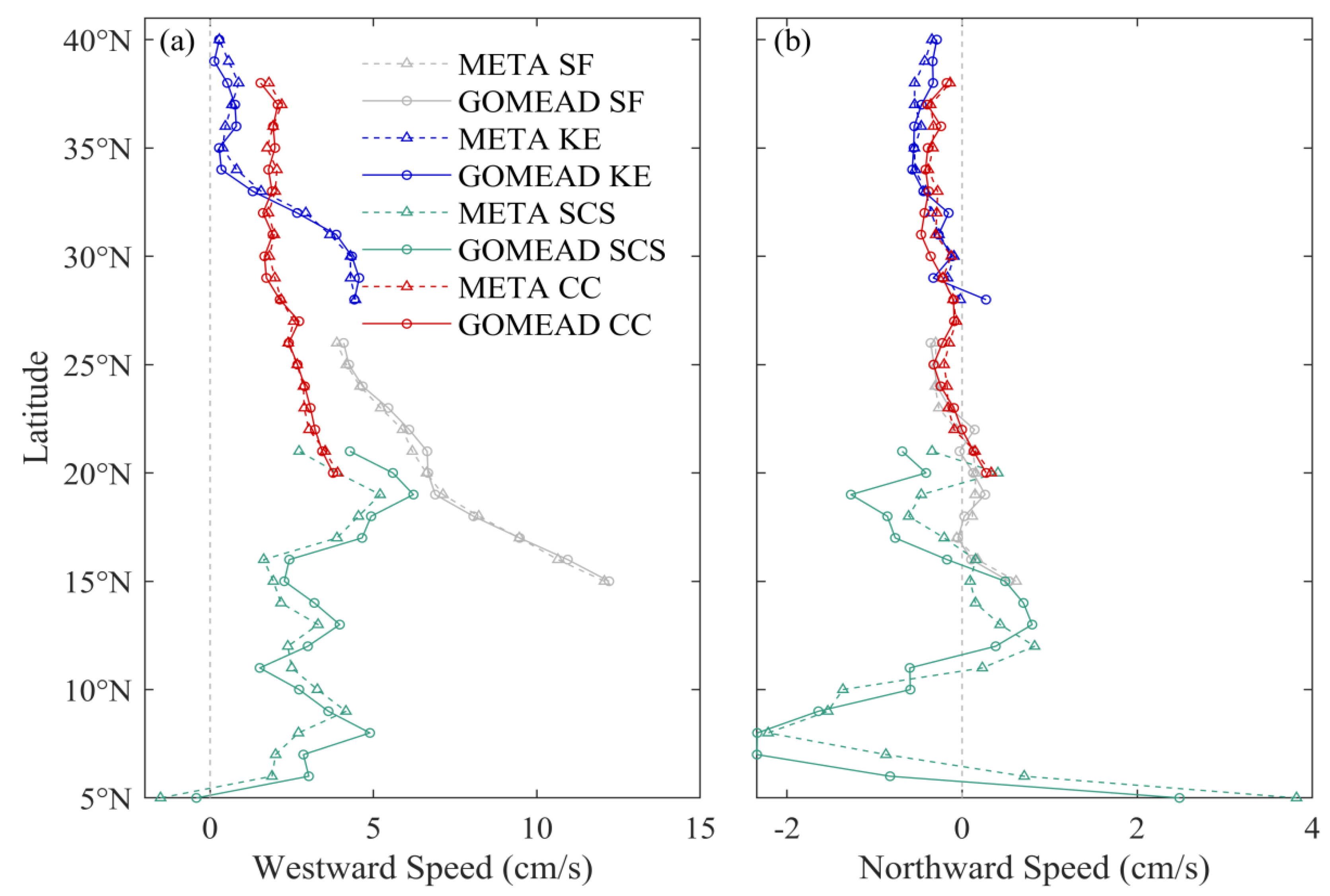
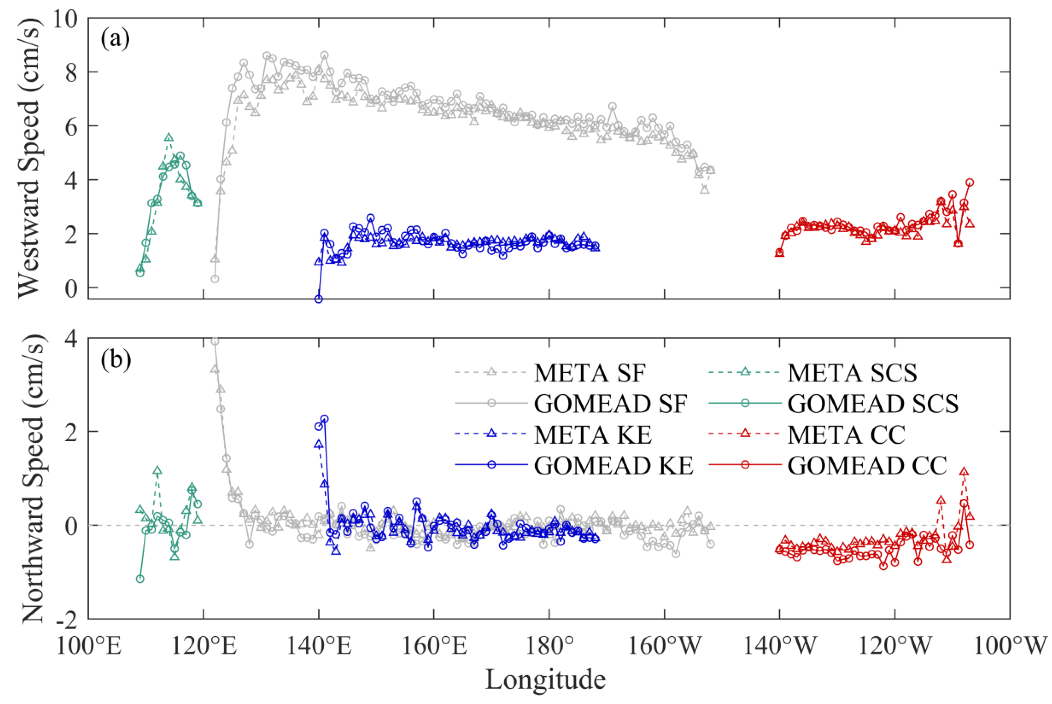
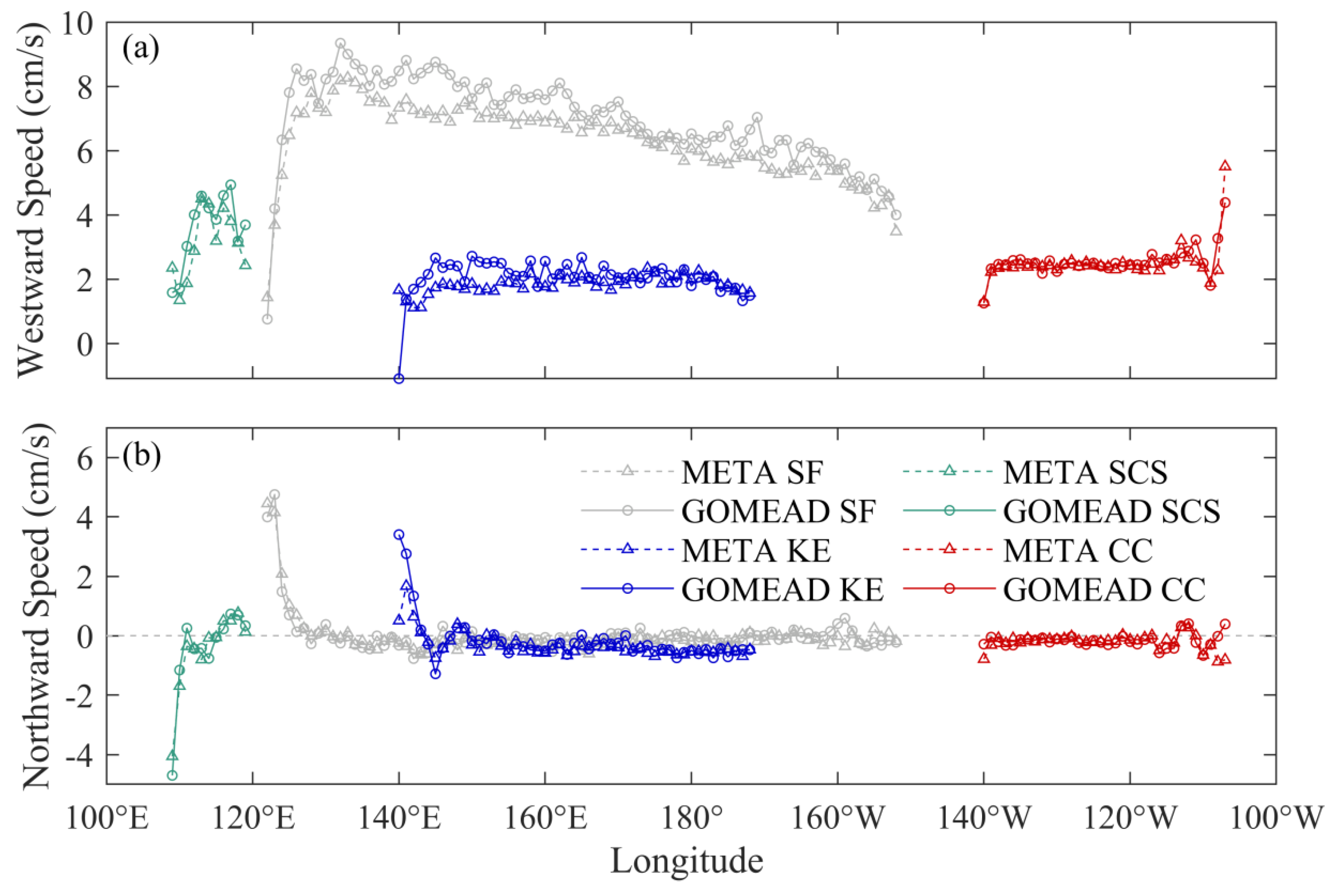
3.5. Eddy Movement
4. Discussion
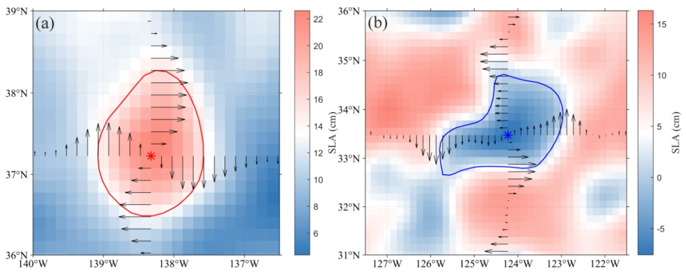
4.1. Eddy Center Difference
4.2. Eddy Number Difference
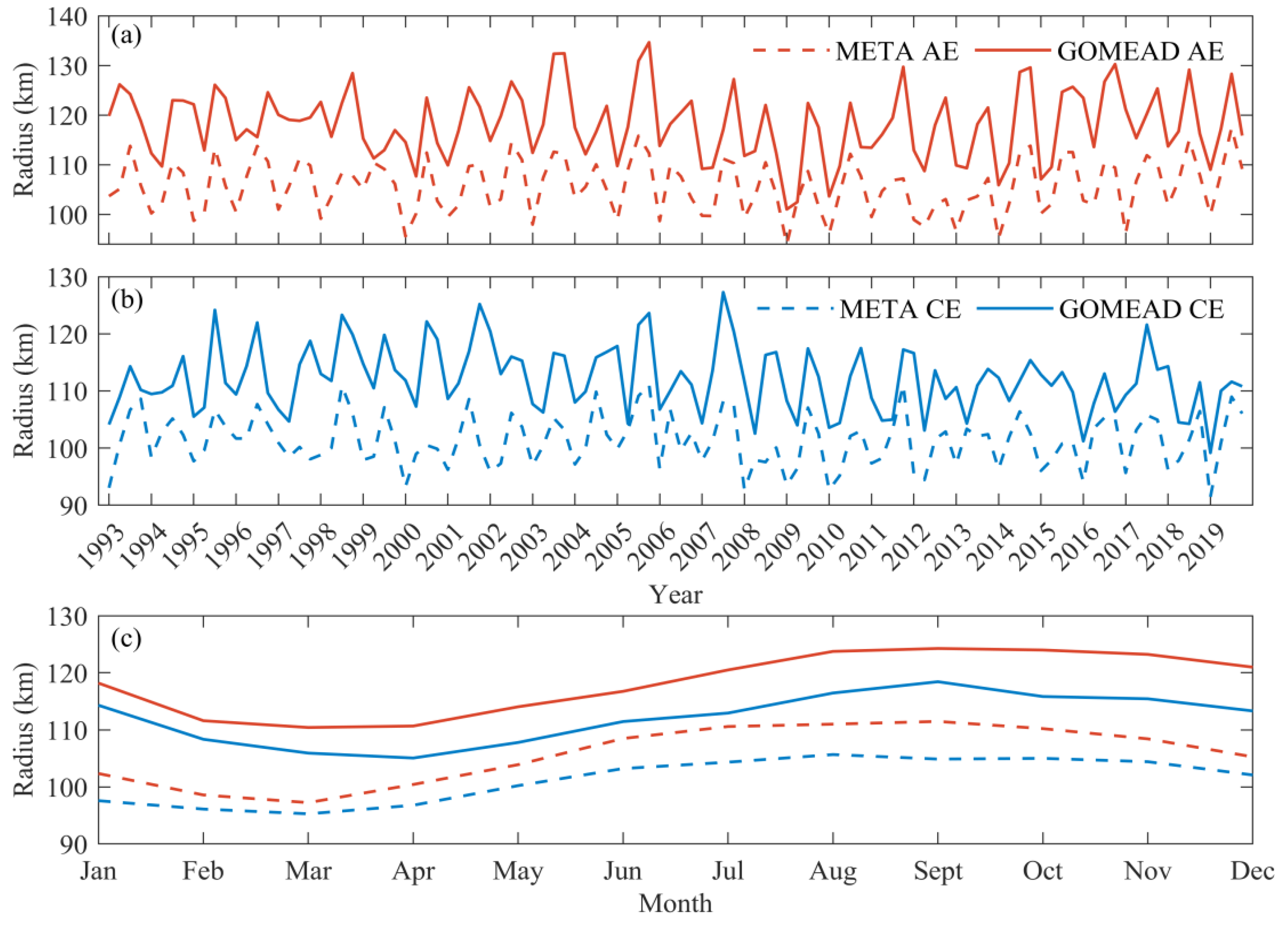
4.3. Eddy Radius Difference
4.4. Eddy Lifespan Difference
5. Conclusions
Author Contributions
Funding
Institutional Review Board Statement
Informed Consent Statement
Data Availability Statement
Acknowledgments
Conflicts of Interest
References
- Chelton, D.B.; Schlax, M.G.; Samelson, R.M.; de Szoeke, R.A. Global observations of large oceanic eddies. Geophys. Res. Lett. 2007, 34, L15606. [Google Scholar] [CrossRef]
- Chelton, D.B.; Schlax, M.G.; Samelson, R.M. Global observations of nonlinear mesoscale eddies. Prog. Oceanogr. 2011, 91, 167–216. [Google Scholar] [CrossRef]
- Frenger, I.; Münnich, M.; Gruber, N.; Knutti, R. Southern ocean eddy phenomenology. J. Geophys. Res. Ocean. 2015, 120, 7413–7449. [Google Scholar] [CrossRef] [Green Version]
- Tian, F.; Wu, D.; Yuan, L.; Chen, G. Impacts of the efficiencies of identification and tracking algorithms on the statistical properties of global mesoscale eddies using merged altimeter data. Int. J. Remote Sens. 2019, 41, 2835–2860. [Google Scholar] [CrossRef]
- Dandapat, S.; Chakraborty, A. Mesoscale eddies in the Western Bay of Bengal as observed from satellite altimetry in 1993–2014: Statistical characteristics, variability and three-dimensional properties. IEEE J. Sel. Top. Appl. Earth Obs. Remote Sens. 2016, 9, 5044–5054. [Google Scholar] [CrossRef]
- Cui, W.; Wang, W.; Zhang, J.; Yang, J. Multicore structures and the splitting and merging of eddies in global oceans from satellite altimeter data. Ocean Sci. 2019, 15, 413–430. [Google Scholar] [CrossRef] [Green Version]
- Li, J.; Liang, Y.; Zhang, J.; Yang, J.; Song, P.; Cui, W. A new automatic oceanic mesoscale eddy detection method using satellite altimeter data based on density clustering. Acta Oceanol. Sin. 2019, 38, 134–141. [Google Scholar] [CrossRef]
- Amores, A.; Monserrat, S.; Melnichenko, O.; Maximenko, N. On the shape of sea level anomaly signal on periphery of mesoscale ocean eddies. Geophys. Res. Lett. 2017, 44, 6926–6932. [Google Scholar] [CrossRef]
- Nencioli, F.; Dong, C.; Dickey, T.; Washburn, L.; McWilliams, J.C. A vector geometry–based eddy detection algorithm and its application to a high-resolution numerical model product and high-frequency radar surface velocities in the Southern California Bight. J. Atmos. Ocean. Technol. 2010, 27, 564–579. [Google Scholar] [CrossRef]
- Halo, I.; Backeberg, B.; Penven, P.; Ansorge, I.; Reason, C.; Ullgren, J.E. Eddy properties in the mozambique channel: A comparison between observations and two numerical ocean circulation models. Deep Sea Res. Part II Top. Stud. Oceanogr. 2014, 100, 38–53. [Google Scholar] [CrossRef]
- Pegliasco, C.; Chaigneau, A.; Morrow, R.; Dumas, F. Detection and tracking of mesoscale eddies in the Mediterranean Sea: A comparison between the Sea Level Anomaly and the Absolute Dynamic Topography fields. Adv. Space Res. 2021, 68, 401–419. [Google Scholar] [CrossRef]
- Sun, W.; Dong, C.; Tan, W.; Liu, Y.; He, Y.; Wang, J. Vertical structure anomalies of oceanic eddies and eddy-induced transports in the South China Sea. Remote Sens. 2018, 10, 795. [Google Scholar] [CrossRef] [Green Version]
- Yi, J.; Du, Y.; He, Z.; Zhou, C. Enhancing the accuracy of automatic eddy detection and the capability of recognizing the multi-core structures from maps of sea level anomaly. Ocean Sci. 2014, 10, 39–48. [Google Scholar] [CrossRef] [Green Version]
- Zhang, C.; Li, H.; Liu, S.; Shao, L.; Zhao, Z.; Liu, H. Automatic detection of oceanic eddies in reanalyzed SST images and its application in the East China Sea. Sci. China Earth Sci. 2015, 58, 2249–2259. [Google Scholar] [CrossRef]
- Le Vu, B.; Stegner, A.; Arsouze, T. Angular momentum eddy detection and tracking algorithm (AMEDA) and its application to coastal eddy formation. J. Atmos. Ocean. Technol. 2018, 35, 739–762. [Google Scholar] [CrossRef]
- Faghmous, J.H.; Frenger, I.; Yao, Y.; Warmka, R.; Lindell, A.; Kumar, V. A daily global mesoscale ocean eddy dataset from satellite altimetry. Sci. Data 2015, 2, 150028. [Google Scholar] [CrossRef] [Green Version]
- Mason, E.; Pascual, A.; McWilliams, J.C. A new sea surface height–based code for oceanic mesoscale eddy tracking. J. Atmos. Ocean. Technol. 2014, 31, 1181–1188. [Google Scholar] [CrossRef] [Green Version]
- Meng, Y.; Liu, H.; Lin, P.; Ding, M.; Dong, C. Oceanic mesoscale eddy in the Kuroshio extension: Comparison of four datasets. Atmos. Ocean. Sci. Lett. 2021, 14, 100011. [Google Scholar] [CrossRef]
- Chaigneau, A.; Gizolme, A.; Grados, C. Mesoscale eddies off Peru in altimeter records: Identification algorithms and eddy spatio-temporal patterns. Prog. Oceanogr. 2008, 79, 106–119. [Google Scholar] [CrossRef]
- Schlax, M.G.; Chelton, D.B. The “Growing Method” of Eddy Identification and Tracking in Two and Three Dimensions. 2016. Available online: https://www.aviso.altimetry.fr/fileadmin/documents/data/products/value-added/Schlax_Chelton_2016.pdf (accessed on 11 November 2021).
- Dilmahamod, A.F.; Aguiar-González, B.; Penven, P.; Reason, C.J.C.; De Ruijter, W.P.M.; Malan, N.; Hermes, J.C. SIDDIES corridor: A major east-west pathway of long-lived surface and subsurface eddies crossing the subtropical south indian ocean. J. Geophys. Res. Ocean. 2018, 123, 5406–5425. [Google Scholar] [CrossRef] [Green Version]
- Gaube, P.J.; McGillicuddy, D.; Moulin, A.J. Mesoscale eddies modulate mixed layer depth globally. Geophys. Res. Lett. 2019, 46, 1505–1512. [Google Scholar] [CrossRef] [Green Version]
- Melnichenko, O.; Hacker, P.; Müller, V. Observations of mesoscale eddies in satellite SSS and inferred eddy salt transport. Remote Sens. 2021, 13, 315. [Google Scholar] [CrossRef]
- Ji, J.; Dong, C.; Zhang, B.; Liu, Y. An oceanic eddy statistical comparison using multiple observational data in the Kuroshio Extension region. Acta Oceanol. Sin. 2017, 36, 1–7. [Google Scholar] [CrossRef]
- Ji, J.; Dong, C.; Zhang, B.; Liu, Y.; Zou, B.; King, G.P.; Xu, G.; Chen, D. Oceanic eddy characteristics and generation mechanisms in the Kuroshio Extension region. J. Geophys. Res. Ocean. 2018, 123, 8548–8567. [Google Scholar] [CrossRef]
- Wang, S.; Zhu, W.; Ma, J.; Ji, J.; Yang, J.; Dong, C. Variability of the Great Whirl and its impacts on atmospheric processes. Remote Sens. 2019, 11, 322. [Google Scholar] [CrossRef] [Green Version]
- Ji, J.; Ma, J.; Dong, C.; Chiang, J.; Chen, D. Regional dependence of atmospheric responses to oceanic eddies in the North Pacific Ocean. Remote Sens. 2020, 12, 1161. [Google Scholar] [CrossRef] [Green Version]
- Dong, C.; Liu, L.; Nencioli, F.; Xia, C.; Xu, G.; Ma, J.; Liu, Y.; Sun, W.; Ji, J. Global Ocean Mesoscale Eddy Atmospheric-Oceanic-Biological Interaction Observational Dataset (GOMEAD) (V1); Science Data Bank: Beijing, China, 2021. [Google Scholar] [CrossRef]
- Couvelard, X.; Caldeira, R.M.A.; Araújo, I.B.; Tomé, R. Wind mediated vorticity-generation and eddy-confinement, leeward of the Madeira Island: 2008 numerical case study. Dynam. Atmos. Ocean. 2012, 58, 128–149. [Google Scholar] [CrossRef]
- Dong, C.; Lin, X.; Liu, Y.; Nencioli, F.; Chao, Y.; Guan, Y.; Chen, D.; Dickey, T.; McWilliams, J.C. Three-dimensional oceanic eddy analysis in the Southern California Bight from a numerical product. J. Geophys. Res. Ocean. 2012, 117, C00H14. [Google Scholar] [CrossRef] [Green Version]
- Liu, Y.; Dong, C.; Guan, Y.; Chen, D.; McWilliams, J.; Nencioli, F. Eddy analysis in the subtropical zonal band of the North Pacific Ocean. Deep Sea Res. Part I Oceanogr. Res. Pap. 2012, 68, 54–67. [Google Scholar] [CrossRef]
- Amores, A.; Monserrat, S.; Marcos, M. Vertical structure and temporal evolution of an anticyclonic eddy in the Balearic Sea (western Mediterranean). J. Geophys. Res. Ocean. 2013, 118, 2097–2106. [Google Scholar] [CrossRef] [Green Version]
- Peliz, A.; Boutov, D.; Teles-Machado, A. The Alboran Sea mesoscale in a long term high resolution simulation: Statistical analysis. Ocean Model. 2013, 72, 32–52. [Google Scholar] [CrossRef]
- Dong, C.; McWilliams, J.C.; Liu, Y.; Chen, D. Global heat and salt transports by eddy movement. Nat. Commun. 2014, 5, 3294. [Google Scholar] [CrossRef] [PubMed] [Green Version]
- Lin, X.; Dong, C.; Chen, D.; Liu, Y.; Yang, J.; Zou, B.; Guan, Y. Three-dimensional properties of mesoscale eddies in the South China Sea based on eddy-resolving model output. Deep Sea Res. Part I 2015, 99, 46–64. [Google Scholar] [CrossRef]
- Qin, D.; Wang, J.; Liu, Y.; Dong, C. Eddy analysis in the Eastern China Sea using altimetry data. Front. Earth Sci. 2015, 9, 709–721. [Google Scholar] [CrossRef]
- Xu, G.; Cheng, C.; Yang, W.; Xie, W.; Kong, L.; Hang, R.; Ma, F.; Dong, C.; Yang, J. Oceanic eddy identification using an AI scheme. Remote Sens. 2019, 11, 1349. [Google Scholar] [CrossRef] [Green Version]
- Yang, X.; Xu, G.; Liu, Y.; Sun, W.; Xia, C.; Dong, C. Multi-source data analysis of mesoscale eddies and their effects on surface chlorophyll in the Bay of Bengal. Remote Sens. 2020, 12, 3485. [Google Scholar] [CrossRef]
- Quattrocchi, G.; Cucco, A.; Cerritelli, G.; Mencacci, R.; Comparetto, G.; Sammartano, D.; Ribotti, A.; Luschi, P. Testing a novel aggregated methodology to assess hydrodynamic impacts on a high-resolution marine turtle trajectory. Front. Mar. Sci. 2021, 8, 699580. [Google Scholar] [CrossRef]
- Liu, Y.; Chen, G.; Sun, M.; Liu, S.; Tian, F. A parallel SLA-based algorithm for global mesoscale eddy identification. J. Atmos. Ocean. Technol. 2016, 33, 2743–2754. [Google Scholar] [CrossRef]
- Kang, L.; Wang, F.; Chen, Y. Eddy generation and evolution in the North Pacific Subtropical Countercurrent (NPSC) zone. Chin. J. Oceanol. Limnol. 2010, 28, 968–973. [Google Scholar] [CrossRef]
- Yoshida, S.; Qiu, B.; Hacker, P. Wind-generated eddy characteristics in the lee of the island of Hawaii. J. Geophys. Res. 2010, 115, C03019. [Google Scholar] [CrossRef]
- Xu, C.; Shang, X.-D.; Huang, R.X. Estimate of eddy energy generation/dissipation rate in the world ocean from altimetry data. Ocean Dynam. 2011, 61, 525–541. [Google Scholar] [CrossRef]
- Zhang, Z.; Tian, J.; Qiu, B.; Zhao, W.; Chang, P.; Wu, D.; Wan, X. Observed 3D structure, generation, and dissipation of oceanic mesoscale eddies in the South China Sea. Sci. Rep. 2016, 6, 24349. [Google Scholar] [CrossRef]
- Chen, G.; Hou, Y.; Zhang, Q.; Chu, X. The eddy pair off eastern Vietnam: Interannual variability and impact on thermohaline structure. Cont. Shelf Res. 2010, 30, 715–723. [Google Scholar] [CrossRef]
- Zhang, Z.; Zhao, W.; Qiu, B.; Tian, J. Anticyclonic eddy sheddings from Kuroshio loop and the accompanying cyclonic eddy in the Northeastern South China Sea. J. Phys. Oceanogr. 2017, 47, 1243–1259. [Google Scholar] [CrossRef] [Green Version]
- Wang, H.; Du, Y.; Liang, F.; Sun, Y.; Yi, J. A census of the 1993–2016 complex mesoscale eddy processes in the South China Sea. Water 2019, 11, 1208. [Google Scholar] [CrossRef] [Green Version]
- Chen, G.; Hou, Y.; Chu, X. Mesoscale eddies in the South China Sea: Mean properties, spatiotemporal variability, and impact on thermohaline structure. J. Geophys. Res. 2011, 116, C06018. [Google Scholar] [CrossRef]
- Xie, J.; De Vos, M.; Bertino, L.; Zhu, J.; Counillon, F. Impact of assimilating altimeter data on eddy characteristics in the South China Sea. Ocean Model. 2020, 155, 101704. [Google Scholar] [CrossRef]
- Xing, T.; Yang, Y. Three mesoscale eddy detection and tracking methods: Assessment for the South China Sea. J. Atmos. Ocean. Technol. 2021, 38, 243–258. [Google Scholar] [CrossRef]
- Zhai, X.; Johnson, H.L.; Marshall, D.P. Significant sink of ocean-eddy energy near western boundaries. Nat. Geosci. 2010, 3, 608–612. [Google Scholar] [CrossRef]
- Zhang, Z.; Wang, W.; Qiu, B. Oceanic mass transport by mesoscale eddies. Science 2014, 345, 322–324. [Google Scholar] [CrossRef]


| META | GOMEAD | |
|---|---|---|
| Raw data | SLA | SLA |
| Data used for detection | SLA | Vector Geometry |
| Resolution | 1/4° | 1/6° |
| Categorization of methods | physical parameter based | geometric velocity field based |
| Eddy center | Centroid | Point of minimum flow speed |
| Eddy edge | Not provided | closed contours with the largest geometric velocity of the stream function |
| Radius | Radius of a circle whose area is equal to that enclosed by the contour of maximum circum-average geostrophic speed | The average distance from the center to each point on the edge of the eddy |
| Amplitude | |SSH (extremum) – SSH (edge)| | It is the same as META (Not directly provided, but can be readily computed) |
| Regions | Latitude | Longitude |
|---|---|---|
| SF | 121°E–150°W | 15°N–28°N |
| KE | 140°E–170°W | 28°N–42°N |
| SCS | 105°E–121°E | 5°N–25°N |
| CC | 105°W–140°W | 20°N–40°N |
| Regions | Parameter (unit) | META | GOMEAD | ||
|---|---|---|---|---|---|
| AE | CE | AE | CE | ||
| SF | Number | 5657 | 6297 | 5443 | 6053 |
| Radius (km) | 97.16 (28.20) | 93.71 (26.94) | 111.01 (38.02) | 107.19 (36.38) | |
| Lifespan (day) | 79.05 (64.87) | 72.62 (54.18) | 66.33 (45.06) | 63.65 (36.40) | |
| Amplitude (cm) | 6.68 (3.69) | 6.87 (3.84) | 7.54 (4.35) | 7.28 (3.86) | |
| KE | Number | 3560 | 3797 | 3402 | 3320 |
| Radius (km) | 80.57 (20.87) | 78.24 (18.76) | 106.71 (38.66) | 104.60 (36.15) | |
| Lifespan (day) | 92.03 (85.87) | 89.62 (80.53) | 69.99 (51.41) | 68.13 (51.13) | |
| Amplitude (cm) | 9.81 (7.28) | 10.14 (8.42) | 13.90 (10.49) | 14.76 (12.87) | |
| SCS | Number | 733 | 855 | 746 | 782 |
| Radius (km) | 109.80 (32.32) | 105.11 (29.75) | 90.43 (23.71) | 89.23 (23.70) | |
| Lifespan (day) | 59.20 (36.09) | 54.65 (29.20) | 57.44 (29.52) | 56.56 (26.61) | |
| Amplitude (cm) | 6.52 (3.96) | 6.34 (3.55) | 4.63 (3.02) | 4.64 (2.64) | |
| CC | Number | 3338 | 3363 | 2800 | 2912 |
| Radius (km) | 74.57 (16.46) | 73.81 (16.41) | 90.36 (28.15) | 92.28 (27.23) | |
| Lifespan (day) | 80.93 (66.52) | 86.75 (77.19) | 66.78 (46.82) | 72.12 (51.92) | |
| Amplitude (cm) | 3.41 (1.77) | 3.81 (2.19) | 4.33 (2.22) | 4.88 (2.72) | |
| Total | Number | 13288 | 14312 | 12391 | 13067 |
| Radius (km) | 87.74 (26.51) | 85.61 (25.05) | 103.93 (36.54) | 102.14 (34.48) | |
| Lifespan (day) | 81.91 (70.77) | 79.38 (67.52) | 66.90 (46.62) | 66.25 (44.03) | |
| Amplitude (cm) | 6.69 (5.19) | 6.99 (5.67) | 8.39 (7.31) | 8.49 (8.09) | |
Publisher’s Note: MDPI stays neutral with regard to jurisdictional claims in published maps and institutional affiliations. |
© 2021 by the authors. Licensee MDPI, Basel, Switzerland. This article is an open access article distributed under the terms and conditions of the Creative Commons Attribution (CC BY) license (https://creativecommons.org/licenses/by/4.0/).
Share and Cite
You, Z.; Liu, L.; Bethel, B.J.; Dong, C. Feature Comparison of Two Mesoscale Eddy Datasets Based on Satellite Altimeter Data. Remote Sens. 2022, 14, 116. https://doi.org/10.3390/rs14010116
You Z, Liu L, Bethel BJ, Dong C. Feature Comparison of Two Mesoscale Eddy Datasets Based on Satellite Altimeter Data. Remote Sensing. 2022; 14(1):116. https://doi.org/10.3390/rs14010116
Chicago/Turabian StyleYou, Zhiwei, Lingxiao Liu, Brandon J. Bethel, and Changming Dong. 2022. "Feature Comparison of Two Mesoscale Eddy Datasets Based on Satellite Altimeter Data" Remote Sensing 14, no. 1: 116. https://doi.org/10.3390/rs14010116
APA StyleYou, Z., Liu, L., Bethel, B. J., & Dong, C. (2022). Feature Comparison of Two Mesoscale Eddy Datasets Based on Satellite Altimeter Data. Remote Sensing, 14(1), 116. https://doi.org/10.3390/rs14010116